Ground state normalization in the nonmesonic weak decay of ${}^{12}_{\Lambda}C$ hypernucleus within a nuclear matter formalism.

Abstract

The nonmesonic weak decay width of ${}^{12}_{\Lambda}C$ hypernucleus has been evaluated within a nuclear matter formalism, using the local density approximation. In addition to the one-body induced decay $(\Lambda N\rightarrow nN)$, it has been also considered the two-body induced decay $(\Lambda NN\rightarrow nNN)$. This second decay is originated from ground state correlations, where a renormalization procedure to ensure a ground state normalized to one has been implemented. Our results show that the plain addition of the two-body induced decay implies a lost in the ground state-norm, which adds $\sim 38\%$ of spurious intensity to the nonmesonic weak decay width. By an adequate selection of the $\Lambda N$-transition potential, our result for the nonmesonic weak decay width of ${}^{12}_{\Lambda}C$ is 0.956, in good agreement with the most recent data.

1 Introduction

A $\Lambda$-hypernucleus decays via the weak interaction mainly by two decay mechanisms: the so-called mesonic decay $(\Lambda\rightarrow\pi N)$ and the nonmesonic one $(NM)$, where no meson is present in the final state (for review articles see [1, 2]). The $NM$-decay width is denoted as $\Gamma_{NM}$, which is defined as the sum of $\Gamma_{1}\equiv\Gamma(\Lambda N\rightarrow nN)$ plus $\Gamma_{2}\equiv\Gamma(\Lambda NN\rightarrow nNN)$. The $\Gamma_{1}$-decay width itself is the sum of $\Gamma_{n}\equiv\Gamma(\Lambda n\rightarrow nn)$ plus $\Gamma_{p}\equiv\Gamma(\Lambda p\rightarrow np)$. Experimental values are given for $\Gamma_{NM}$, the ratio $\Gamma_{n/p}\equiv\Gamma_{n}/\Gamma_{p}$ and the asymmetry of the protons emitted in the $NM$ decay of polarized hypernuclei. In the present contribution, we focuss on $\Gamma_{NM}$, evaluated in nuclear matter together with the local density approximation which allows us to analyze the ${}^{12}_{\Lambda}C$ hypernucleus.

In the past, it has been an usual statement to assert that while the theory accounts for the experimental values of $\Gamma_{NM}$, the same is not true for the ratio $\Gamma_{n/p}$. In fact, the disagreement between the theoretical and the experimental value for this ratio, has been named as ”the $\Gamma_{n/p}$-puzzle”. This situation has changed in recent years: new theoretical analysis together with more experimental information, have led us to a solution of the so-called puzzle. A typical theoretical value for the ratio for ${}^{12}_{\Lambda}C$ is $\Gamma_{n/p}\sim 0.3$, while data analyzed by means of the intranuclear cascade code (INC) [3, 4, 5, 6], gives a result $\Gamma_{n/p}^{exp}\sim 0.4\pm 0.1$. However, it should be noted that there still exist discrepancies with some nucleon spectra. For instance, the experimental single coincidence proton spectra for ${}^{12}_{\Lambda}C$ is not well reproduced yet.

In nuclear matter (using the local density approximation), some reported calculations for $\Gamma_{1}$ for ${}^{12}_{\Lambda}C$, have values in the range between 0.5 [7] up to 1.45 [8] (given in units of the $\Lambda$-free decay width, $\Gamma^{0}$). While typically $\Gamma_{2}/\Gamma_{1}\sim 0.3$. The most recent experimental determination of $\Gamma_{NM}$ has been done by Outa et al. [9], whom have reported a value $\Gamma_{NM}^{exp}=0.940\pm 0.035$. Some previous experimental determinations are $\Gamma_{NM}^{exp}=1.14\pm 0.20$ [10], $\Gamma_{NM}^{exp}=0.89\pm 0.15\pm 0.03$ [11] and $\Gamma_{NM}^{exp}=0.828\pm 0.056\pm 0.066$ [12]. There is some incompatibility between the result in [12], due to Sato et al. and both Noumi et al. [11] and Outa et al. We have relied on the Outa result, not only because it is the most recent one, but also due to it compatibility with both [10] and [11]-values. Beyond this controversy, the more precise determination of $\Gamma_{NM}^{exp}$ offers us the opportunity to revise the theoretical determination of $\Gamma_{NM}$. In two previous works, a model for the evaluation of $\Gamma_{1}$ and $\Gamma_{2}$ have been developed (see [13] and [14], respectively). Our scheme employs the same microscopic formalism and interactions for both $\Gamma_{1}$ and $\Gamma_{2}$. Within this model, the reproduction of $\Gamma_{NM}^{exp}$ seems not possible: the predicted values are always too big. The main concern of this work is to understand and solve this problem.

To solve this problem it has been revised the way in which $\Gamma_{2}$ is added to $\Gamma_{1}$, to build up $\Gamma_{NM}$. The $\Gamma_{2}$-contribution is originated from ground state correlations and the simple addition of $\Gamma_{2}$ plus $\Gamma_{1}$, would add some spurious intensity because the ground state is not normalized to one. This point turns out to be relevant not only in the determination of $\Gamma_{NM}$, but also for the $\Gamma_{2}/\Gamma_{1}$-ratio, which is used as an input in the determination of $\Gamma_{n/p}^{exp}$. As a further comment on this point, the lack in the normalization is not restricted to our particular model, but to any calculation where $\Gamma_{2}$ is considered. A second point refers to the implementation of short range correlations ($SRC$) in nuclear matter. It is shown that for $\Gamma_{2}$ this has to be done with some particular care due to numerical reasons. The implementation of these two points in the already developed formalism for $\Gamma_{1}$ and $\Gamma_{2}$, gives a $\Gamma_{NM}$-value in good agreement with data.

This work is organized as follows. In Sect. 2, our model for the renormalization of the ground state is presented, showing a scheme to add $\Gamma_{2}$ to $\Gamma_{NM}$. In Sect. 3, a model for the $SRC$ in nuclear matter is discussed in detail. Numerical results are shown in Sect. 4, together with an analysis of the implications of the corrections. Finally, in Sect. 5, some conclusions are given.

2 Ground state correlations ($GSC$)

To start with, we write down the partial decay width $\Gamma_{NM}(k_{F})$ in a schematic way as,

$$\Gamma_{NM}(k_{F})=\sum_{f}\,|\langle f|V^{\Lambda N}|0\rangle_{k_{F}}|^{2}\delta^{(4)}(p_{f}-p_{0}),$$ (1)

where $|0\rangle_{k_{F}}$ and $|f\rangle$ are the ground state and the final state, respectively; $V^{\Lambda N}$ is the two-body transition potential and $p_{i}$ represents an energy-momentum four-vector. The Fermi momentum is denoted as $k_{F}$. By performing the integration over $k_{F}$ using the local density approximation (see [8]), the total decay width $\Gamma_{NM}$ is obtained. Now, the ground state can be written as,

$$|0\rangle_{k_{F}}={\cal N}(k_{F})\,\left(|\;\rangle_{k_{F}}-\frac{1}{4}\,\sum_{p_{1},p_{2},h_{1},h_{2}}\,\frac{\langle p_{1}p_{2}h_{1}h_{2}|V^{NN}|\;\rangle_{k_{F}}}{\epsilon_{p1}+\epsilon_{p2}-\epsilon_{h1}-\epsilon_{h2}}\,|p_{1}p_{2}h_{1}h_{2}\rangle\right),$$ (2)

where the second term in the right hand side of the equation represents $2p2h$-correlations. In this equation $|\;\rangle_{k_{F}}$, is the Hartree-Fock vacuum. In the denominator, $\epsilon_{i}$ are the single particle energies. The nuclear residual interaction is represented by $V^{NN}$ and ${\cal N}(k_{F})$ is the normalization as a function of $k_{F}$:

$${\cal N}(k_{F})=\left(1+\frac{1}{16}\,\sum_{p_{1},p_{2},h_{1},h_{2}}\,\left|\frac{\langle p_{1}p_{2}h_{1}h_{2}|V^{NN}|\;\rangle_{k_{F}}}{\epsilon_{p1}+\epsilon_{p2}-\epsilon_{h1}-\epsilon_{h2}}\right|^{2}\,\right)^{-1/2}.$$ (3)

We will show soon that the inclusion of ${\cal N}(k_{F})$, has an important effect over $\Gamma_{NM}$. The importance of a proper treatment of the ground state normalization has been already pointed out by Van Neck et al. [15]. When Eq. (2) is inserted into the expression of $\Gamma_{NM}(k_{F})$ given by Eq. (1) with the arbitrary selection of ${\cal N}(k_{F})=1$, the usual expressions for $\Gamma_{1}$ and $\Gamma_{2}$, are obtained. The first one comes from the first term in Eq. (2), while $\Gamma_{2}$ results from the second term in the same equation.

Alternatively, if the $GSC$ are neglected (i.e. $\Gamma_{2}=0$), then $|0\rangle_{k_{F}}=|\;\rangle_{k_{F}}$ and ${\cal N}(k_{F})=1$. However, when $GSC$ are included, the use of ${\cal N}(k_{F})=1$ means that the ground state is not properly normalized and therefore some spurious intensity is added to $\Gamma_{NM}$.

3 Short range correlations ($SRC$)

In momentum space one model to take care of $SRC$ is by the use of a modified transition potential obtained as, (see [16]),

$$V_{SRC}(\mbox{\boldmath$q$})\,=\,V(\mbox{\boldmath$q$})\,-\,\int\frac{d\mbox{\boldmath$p$}}{(2\pi)^{3}}\tilde{\xi}(|\mbox{\boldmath$p$}+\mbox{\boldmath$q$}|)\,V(\mbox{\boldmath$p$}),$$ (4)

where we employ,

$$\tilde{\xi}(p)=\frac{2\pi^{2}}{q_{c}^{2}}\,\delta(p-q_{c}),$$ (5)

with $q_{c}=780$ MeV/c, as a particular correlation function in momentum space. We have limited our discussion of $SRC$ to this model and it implementation in the evaluation of $\Gamma_{NM}$ deserves some care. We show this with an example. Let us show the result of Eq. (4) with the central part of the parity conserving one pion exchange potential, which we write in a simplified manner as,

$$V_{\pi}^{C}(\mbox{\boldmath$q$})=C_{\pi}\;\frac{\mbox{\boldmath$q$}^{2}}{\mbox{\boldmath$q$}^{2}+m_{\pi}^{2}}\mbox{\boldmath$\sigma_{1}$}\cdot\mbox{\boldmath$\sigma_{2}$}\;\mbox{\boldmath$\tau_{1}$}\cdot\mbox{\boldmath$\tau_{2}$}$$ (6)

with $C_{\pi}=-G_{F}m_{\pi}^{2}\;(g_{NN\pi}/2M)\;(B_{\pi}/2\bar{M})$, where $\bar{M}$, is the average between the nucleon and $\Lambda$ masses. Using this potential in Eq. (4) we obtain,

$$V_{\pi}^{SRC,\,C}(\mbox{\boldmath$q$}) =\,V_{\pi}^{C}(\mbox{\boldmath$q$})\,-$$ (7)

$$C_{\pi}\frac{1}{2}\{2+\frac{m_{\pi}^{2}}{2q_{c}|\mbox{\boldmath$q$}|}\ln|\frac{q_{c}^{2}+m_{\pi}^{2}+\mbox{\boldmath$q$}^{2}-2q_{c}|\mbox{\boldmath$q$}|}{q_{c}^{2}+m_{\pi}^{2}+\mbox{\boldmath$q$}^{2}+2q_{c}|\mbox{\boldmath$q$}|}|\}\mbox{\boldmath$\sigma_{1}$}\cdot\mbox{\boldmath$\sigma_{2}$}\;\mbox{\boldmath$\tau_{1}$}\cdot\mbox{\boldmath$\tau_{2}$}$$

by calling $\kappa=2q_{c}|\mbox{\boldmath$q$}|/(q_{c}^{2}+m_{\pi}^{2}+\mbox{\boldmath$q$}^{2})$ and making the approximation,

$$\ln(1+\kappa)\approx\kappa$$ (8)

we finally obtain,

$$V_{\pi}^{SRC,\,C}(\mbox{\boldmath$q$})\,=\,V_{\pi}^{C}(\mbox{\boldmath$q$})\,-\,C_{\pi}\frac{q_{c}^{2}+\mbox{\boldmath$q$}^{2}}{q_{c}^{2}+m_{\pi}^{2}+\mbox{\boldmath$q$}^{2}}\mbox{\boldmath$\sigma_{1}$}\cdot\mbox{\boldmath$\sigma_{2}$}\;\mbox{\boldmath$\tau_{1}$}\cdot\mbox{\boldmath$\tau_{2}$}$$ (9)

which is equivalent to the following general prescription to build up the modified potential due to the action of the $SRC$:

$$V^{SRC,\,C}(\mbox{\boldmath$q$})\,=\,V^{C}(\mbox{\boldmath$q$})\,-V^{C}(\mbox{\boldmath$q$}^{2}\rightarrow q_{c}^{2}+\mbox{\boldmath$q$}^{2}).$$ (10)

To the best of our knowledge, this way of taking care of $SRC$ in nuclear matter is the most frequently used one. However, we should call attention on the non-equivalence between the approximation in Eq. (10) and the one in Eq. (4) for the kinematical conditions of the nonmesonic $\Lambda$-decay. This is because the approximation given by Eq. (8), is a bad approximation for the momentum transfer in the $\Lambda N\rightarrow NN$ decay channel (where $q\approx 400$ MeV/c). A simple numerical test shows that Eq. (10) fairly accounts for the expression given by Eq. (4) only for $q\lesssim 50$ MeV/c. For the full $V^{\Lambda N}$-transition potential (which includes $q$-dependent form factors), the integral in Eq. (4) can be also performed analytically. The numerical results show that $\Gamma_{NM}$ evaluated with the inclusion of $SRC$ given by the model in Eqs. (4) and (5), is $\sim 35\%$ smaller than the same quantity with the prescription in Eq. (10) (employing the same $q_{c}$-value). In the present contribution we present results only for the model in Eqs. (4) and (5), as this model gives us some confidence about it applicability within a wide range in the variation of the momentum transfer.

Due to it frequent use, it is important to discuss the prescription in Eq. (10), which is in fact, an approximation to the model in Eqs. (4) and (5). The employment of this prescription would be particularly questionable in the evaluation of $\Gamma_{2}$ (rather than $\Gamma_{1}$), for the reasons that follows. Let us write down explicit expressions for both $\Gamma_{1}$ and $\Gamma_{2}$. We do this in a very schematic way,

$$\Gamma_{1}(\mbox{\boldmath$k$},k_{F})=C\int d\mbox{\boldmath$q$}\theta(q_{0})\theta(|\mbox{\boldmath$k$}-\mbox{\boldmath$q$}|-k_{F})(V^{\Lambda N}(q))^{SRC}Im\Pi_{1p1p}(q_{0},\mbox{\boldmath$q$})$$ (11)

and

$$\Gamma_{2}(\mbox{\boldmath$k$},k_{F})=C\int d\mbox{\boldmath$q$}\theta(q_{0})\theta(|\mbox{\boldmath$k$}-\mbox{\boldmath$q$}|-k_{F})(V^{\Lambda N}(q))^{SRC}Im\Pi_{2p2p}(q_{0},\mbox{\boldmath$q$})$$ (12)

where $C=-6(G_{F}m_{\pi}^{2})^{2}\pi/(2\pi)^{3}$ and $q_{0}=k_{0}-E(\mbox{\boldmath$k$}-\mbox{\boldmath$q$})-V_{N}$, being $k$ the energy-momentum of the $\Lambda$. Final values for $\Gamma_{1}$ and $\Gamma_{2}$ are obtained after integrating over $k$ and $k_{F}$. The functions $\Pi_{1p1p}$ and $\Pi_{2p2p}$ are the $1p1h$ and $2p2h$-polarizations functions, respectively. We do not go through the derivation of these expressions (details can be found in [17], for instance).

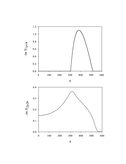
Figure 1: Imaginary part of the polarization functions $\Pi_{1p1h}$ and $\Pi_{2p2h}$ as a function of the momentum transfer $q$. The polarization functions and $q$, are in units of $10^{-3}$ MeV^-1 fm^-3 and MeV/c, respectively.

In Fig. 1, we have plotted $Im\Pi_{1p1p}$ and $Im\Pi_{2p2p}$ as a function of the momentum transfer $q$. For simplicity, this is done for a $\Lambda$ at rest ($\mbox{\boldmath$k$}=0$) and for $k_{F}=210$ MeV/c. The behavior of $Im\Pi_{1p1p}$, is a narrow function, peaked around $q\approx 400$ MeV/c. This range of variation in $q$, makes the approximation in Eq. (10) acceptable once $q_{c}$ is somehow adjusted. Let us be clear: with the same $q_{c}$-value, the results from Eq. (4) and Eq. (10) are different because $Im\Pi_{1p1p}$ is non-zero far way from $q\lesssim 50$ MeV/c. But the narrow $q$-variation establish by $Im\Pi_{1p1p}$, would make the approximation in Eq. (10) acceptable, once the $q_{c}$-value is adjusted using some observable or by a comparison with a finite nucleus calculation.

From the same figure, the situation for $Im\Pi_{2p2p}$ is very different as it is spread over a wide $q$-region. The use of Eq. (10) would introduce a systematic error in the evaluation of $\Gamma_{2}$, because due to a numerically wrong approximation, the $SRC$ are incorrectly weighed for different $q$-values. This warning is not restricted to our particular $\Gamma_{2}$-evaluation. There are two former models for the evaluation of $\Gamma_{2}$. The starting point of all this evaluations (together with the one of ours) is the Eq. (12), but they differ between each other in the model for $\Pi_{2p2h}$. The first work which has called attention on $\Gamma_{2}$ is the one due to Alberico et al. [18], where a so-called semi-phenomenological $\Gamma_{2}$ has been adopted, which results from a microscopic evaluation of the polarization propagator $\Pi_{2p2h}$ in nuclear matter, originally performed for electron scattering in [19]. Using this electron scattering calculation, a constant $Im\Pi_{2p2h}$ is proposed, which is appropriate for pion absorption. Thereafter, Ramos et al. [17], has used also a semi-phenomenological $\Gamma_{2}$, where an approximate value for the function $Im\Pi_{2p2h}$, is obtained as the product of the phase space corresponding to the $\Lambda NN\rightarrow NNN$-reaction, times a constant taken from pion absorption. It should be noted that in the $\Lambda NN\rightarrow NNN$-reaction, all mesons are strictly off the mass shell and the employment of the pion absorption results are used as an approximation to take care of the dynamics involved in the evaluation of $\Gamma_{2}$. Beyond the same starting point of Eq. (12) and the difference in the calculation of the function $Im\Pi_{2p2h}$, these two works also differ from the one in [14], by the way in which the isospin is taken into consideration and some minor points. In any case, the just quoted warning in the inclusion of the $SRC$ is valid for all these $\Gamma_{2}$-models.

4 Results and discussion

We turn now to the numerical results. The transition potential $V^{\Lambda N}$, is represented by the exchanges of the $\pi$, $\eta$, $K$, $\rho$, $\omega$ and $K^{*}$-mesons, whose formulation has been taken from [20], and the values of the different coupling constants and cutoff parameters appearing in the transition potential have been taken from [21] and [22], named as Nijimegen and NSC97f, respectively. For the nuclear residual interaction $V^{NN}$ (which is employed in both $\Gamma_{2}$ and ${\cal N}(k_{F})$), we have used the Bonn potential [23] in the framework of the parametrization presented in [24], which contains the exchange of $\pi$, $\rho$, $\sigma$ and $\omega$ mesons, while the $\eta$ and $\delta$-mesons are neglected. In implementing the LDA, the hyperon is assumed to be in the $1s_{1/2}$ orbit of a harmonic oscillator well with frequency $\hbar\omega=10.8$ MeV, where we have employed different values for the proton and neutron Fermi momenta, $k_{F_{n}}$ and $k_{F_{p}}$, respectively (for details see [25]).

The partial decay widths $\Gamma_{1}(k_{F})$ and $\Gamma_{2}(k_{F})$ have been evaluated using the scheme developed in [13] and [14], respectively; but with the implementation of the $SRC$ described above. The $\Gamma_{2}$-contribution is built up to three terms: $\Gamma_{2}=\Gamma_{nn}+\Gamma_{np}+\Gamma_{pp}$, with $\Gamma_{nn}\equiv\Gamma(\Lambda nn\rightarrow nnn)$, $\Gamma_{np}\equiv\Gamma(\Lambda np\rightarrow nnp)$ and $\Gamma_{pp}\equiv\Gamma(\Lambda pp\rightarrow npp)$. The dominant term is $\Gamma_{np}$, where the relative magnitude of each contribution follows approximately the relation, $\Gamma_{np}:\Gamma_{pp}:\Gamma_{nn}\approx 0.78:0.17:0.05$. It should be noted that once the $GSC$ are considered, the partial decay widths $\Gamma_{1}(k_{F})$ and $\Gamma_{2}(k_{F})$ are multiplied by the function ${\cal N}(k_{F})$ and then, the $k_{F}$-integration gives the final $\Gamma_{NM}$. Therefore, the action of the ground state renormalization is not the plain multiplication of $\Gamma_{1,\,2}$ by a constant. In this procedure, we have employed the same nuclear matter model for $\Gamma_{1,\,2}(k_{F})$ and ${\cal N}(k_{F})$, using the same nuclear residual interaction, transition potential and the $SRC$-model.

In Table 1, we present our values for $\Gamma_{1,\ 2}$ and $\Gamma_{NM}$ for the two mentioned sets of transition potential parameters, with and without the action of ${\cal N}(k_{F})$. In first place, it is clear that the effect of the ground state renormalization is important: for both interactions, the spurious part in $\Gamma_{NM}$ (i.e. $100\times|\Gamma_{NM}(without\;renorm.)-\Gamma_{NM}(with\;renorm.)|/\Gamma_{NM}(with\;renorm.)$), is $\sim 38\%$. At variance, the $\Gamma_{1}$ without renormalization does not differ very much from $\Gamma_{NM}$ ($=\Gamma_{1}+\Gamma_{2}$) with renormalization. Our final $\Gamma_{NM}$ with renormalization shows a small decrease (increase) with respect to $\Gamma_{1}$ without renormalization, for the interaction Nijimegen (NSC97f). In fact, while for Nijimegen the value for $\Gamma_{1}$ is greater than the same one for NSC97f; just the opposite occurs for $\Gamma_{2}$. This is a consequence of the different weight of each spin-isospin component in each interaction, together with the different structure in the spin-isospin sums between $\Gamma_{1}$ and $\Gamma_{2}$. As a further point for this paragraph, our $\Gamma_{NM}$-result for the interaction Nijimegen is in close agreement with the data from [9]. And so does the result for the interaction NSC97f with the data from [12]. Although both data have been included in the table, for the reasons already discussed we rely on the [9] data and therefore, we consider the $\Gamma_{NM}=0.956$ value as our final result. Consequently, the $\Gamma_{2}/\Gamma_{1}$-ratio takes a value 0.28. It should be stressed that the $\Gamma_{2}$-contribution represents $22-30\%$ of $\Gamma_{NM}$ and while there are many theoretical works which deals with the evaluation of $\Gamma_{1}$, the same does not occur for $\Gamma_{2}$.

Table 1: The nonmesonic weak decay width of ${}^{12}_{\Lambda}C$. The first column represents the $V^{\Lambda N}$-transition potential and the second one refers to the inclusion or not of the normalization factor in the ground state. All $\Gamma$’s are in units of free $\Lambda$-decay rate, $\Gamma^{0}=2.52\cdot 10^{-6}$ eV.

$model\;int.$	$renorm.$	${\Gamma}_{1}$	${\Gamma}_{2}$	${\Gamma}_{NM}$
Nijimegen  [21]	$no$	1.031	0.289	1.320
NSC97f  [22]	$no$	0.814	0.348	1.162
Nijimegen  [21]	$yes$	0.747	0.209	0.956
NSC97f  [22]	$yes$	0.590	0.250	0.840
experiment  [9]				$0.940\pm 0.035$
experiment  [12]				$0.828\pm 0.056\pm 0.066$

In Table 2, a similar analysis to the one in Table 1, is done for ${\Gamma}_{n,\,p}$ and the ratio ${\Gamma}_{n/p}$, where the theoretical values are obtained with the scheme in [13], (but using the oscillator frequency $\hbar\omega=10.8$ MeV, just mentioned). The decay widths ${\Gamma}_{n,\,p,\,nn\,...}$ are primary decays. This means that to extract the ratio ${\Gamma}^{exp}_{n/p}$, from the experimental spectra, a model for the analysis of data is required, where the $\Gamma_{2}/\Gamma_{1}$-ratio plays an important role. This point is further discussed in the next paragraphs. In the present table, two experimental values are shown: the one from Outa et al. [9], whom have used the approximation $N_{nn}/N_{np}\simeq\Gamma_{n}/\Gamma_{p}$, where $N_{ij}$ represents the total number of $ij$-pairs emitted in the $\Lambda$-weak decay (this result is denoted as preliminary by the author). In this table it is also reported the value by Sato et al. [12], that has been extracted under the assumption of $\Gamma_{2}/\Gamma_{1}=0.35$ and obtained from single-proton energy spectra. These $\Gamma_{n/p}^{exp}$-values are consistent with the above reported one ($\Gamma_{n/p}^{exp}\sim 0.4\pm 0.1$). In this table, it is also observed that the ratio ${\Gamma}_{n/p}$ is roughly unaffected by the renormalization procedure.

Table 2: The same as Table 1, but for ${\Gamma}_{n}$, ${\Gamma}_{p}$ and the ratio $\Gamma_{n}/\Gamma_{p}$.

$model\;int.$	$renorm.$	${\Gamma}_{n}$	${\Gamma}_{p}$	${\Gamma}_{n}/{\Gamma}_{p}$
Nijimegen  [21]	$no$	0.213	0.819	0.260
NSC97f  [22]	$no$	0.155	0.660	0.235
Nijimegen  [21]	$yes$	0.154	0.593	0.260
NSC97f  [22]	$yes$	0.112	0.478	0.234
experiment  [9]				$0.56\pm 0.12\pm 0.04$
experiment  [12]				$0.60^{+0.11+0.23}_{-0.09-0.21}$

Before going on, we give a brief overview of how the values of $\Gamma_{NM}$ and $\Gamma_{n}/\Gamma_{p}$ are extracted from data. In first place, the hypernuclear weak decay lifetime $\tau$, is an observable which is related to the total decay width $\Gamma_{tot}$, as follows,

$$\tau=\frac{\hbar}{\Gamma_{tot}},$$ (13)

where $\Gamma_{tot}=\Gamma_{M}+\Gamma_{NM}$, with $\Gamma_{M}$ being the mesonic decay width. The evaluation of $\Gamma_{M}$ is less controversial than the non-mesonic decay width, which gives us some confidence on the experimental value for $\Gamma_{NM}$.

The extraction of the $\Gamma_{n}/\Gamma_{p}$-ratio from data is much more involved. This is because both $\Gamma_{n}$ and $\Gamma_{p}$, are primary decays, which implies that they take place within the nucleus and can not be directly measured. The magnitudes which can be measured are the number of neutrons (protons) emitted as a consequence of the $\Lambda$-decay, denoted as $N_{n}$ ($N_{p}$) or also the number of neutron-neutron (neutron-proton) pairs, named as $N_{nn}$ ($N_{np}$). Moreover, these numbers are measured within certain energy-intervals, which allows us to draw the particle spectra. There are several ways to connect $N_{n}$ and $N_{p}$ (or $N_{nn}$ and $N_{np}$), with $\Gamma_{n}$ and $\Gamma_{p}$. One of them is the INC, which is briefly discussed. The INC is one of the most sophisticated models to extract this ratio from data. Within this model, the $N_{n}/N_{p}$-ratio is related to the $\Gamma_{n}/\Gamma_{p}$-ratio through the following relation [5],

$$\frac{N_{n}}{N_{p}}=\frac{N^{\rm 1Bn}_{n}\displaystyle\frac{\Gamma_{n}}{\Gamma_{p}}+N^{\rm 1Bp}_{n}+N^{\rm 2B}_{n}\left(1+\frac{\Gamma_{n}}{\Gamma_{p}}\right)\frac{\Gamma_{2}}{\Gamma_{1}}}{N^{\rm 1Bn}_{p}\displaystyle\frac{\Gamma_{n}}{\Gamma_{p}}+N^{\rm 1Bp}_{p}+N^{\rm 2B}_{p}\left(1+\frac{\Gamma_{n}}{\Gamma_{p}}\right)\frac{\Gamma_{2}}{\Gamma_{1}}}\,,$$ (14)

with an analogous expression for $N_{nn}/N_{np}$. The quantities $N^{\rm 1Bi}_{k}$ and $N^{\rm 2B}_{k}$ are numerically evaluated within the INC and are independent of the weak-vertex. To extract $\Gamma_{n/p}^{exp}$ from this expression one has to assume a particular value for the $\Gamma_{2}/\Gamma_{1}$-ratio. For instance, in [6] the results are: $\Gamma_{n/p}^{exp}=0.43\pm 0.10$ for $\Gamma_{2}/\Gamma_{1}=0.26$ and $\Gamma_{n/p}^{exp}=0.46\pm 0.09$ for $\Gamma_{2}/\Gamma_{1}=0.$ As mentioned, the INC is one model in the data analysis. In the work done by Sato et al. [12], it is reported $\Gamma_{n/p}^{exp}=0.60^{+0.11+0.23}_{-0.09-0.21}$ for $\Gamma_{2}/\Gamma_{1}=0.35$, while $\Gamma_{n/p}^{exp}=0.87\pm 0.09\pm 0.21$ for $\Gamma_{2}/\Gamma_{1}=0$. These results are obtained by a Monte-Carlo simulation based on GEANT [26] and the INC from [3], by fitting single-proton energy spectra and using the $\Gamma_{n/p}$-ratio as a free parameter. Let us mention that in [25] and [27], a microscopic model for the spectra itself has been developed, where the primary decays $\Gamma_{n}$ and $\Gamma_{p}$ are one ingredient within the full calculation. From this point of view, it is the nucleon emission spectra, rather than the $\Gamma_{n/p}$-ratio, the magnitude which should be compared with data.

From these last two paragraphs we have tried to call attention on the fact that the accurate determination of both $\Gamma_{1}$ and $\Gamma_{2}$ are equally important. We resume now some of the more frequent approaches on this subject:

• Only $\Gamma_{1}$ is evaluated, while the phase space for $\Gamma_{2}$ is considered, taking the $\Gamma_{2}/\Gamma_{1}$-ratio as a free parameter. In this case, the dynamics in $\Gamma_{2}$ is not evaluated. A comparison of both $\Gamma_{NM}$ and $\Gamma_{n/p}$ with data is questionable as the $\Gamma_{2}$ component is arbitrarily varied to achieve the best match with data. Up to now, from the experimental point of view, it is not possible to disentangle the individual magnitudes of $\Gamma_{1}$ and $\Gamma_{2}$ in $\Gamma_{NM}$. As the magnitude of $\Gamma_{2}$ is sizable compared with $\Gamma_{1}$, there is no ground to avoid the explicit evaluation of $\Gamma_{2}$. Note that a not-null $\Gamma_{2}$ implies a correlated ground state, which alters the $\Gamma_{1}$ itself.

• Both $\Gamma_{1}$ and $\Gamma_{2}$ are evaluated in nuclear matter, without renormalization. In this case, the problem is the simultaneous reproduction of both $\Gamma_{NM}^{exp}$ and $\Gamma_{n/p}^{exp}$. If we care about $\Gamma_{NM}^{exp}$, the wide range of variation in the reported values for $\Gamma_{1}$ and $\Gamma_{2}$, allows to accomplish also a good agreement with data for $\Gamma_{NM}$, but with wrong values for $\Gamma_{1}$ and $\Gamma_{2}$, although the sum is correct. In this case, a small $\Gamma_{1}$ is compensated by some spurious intensity added by $\Gamma_{2}$. This mistake is not harmless as an incorrect ratio $\Gamma_{2}/\Gamma_{1}$ would lead to a wrong analysis of data and an inappropriate choice for the transition potential parametrization, which would affect the whole theoretical calculation. On the other hand, if we focus on $\Gamma_{n/p}^{exp}$, the theoretical $\Gamma_{NM}$ will certainly overestimate $\Gamma_{NM}^{exp}$.

• The $\Gamma_{1}$ decay is evaluated in finite nucleus while $\Gamma_{2}$ in evaluated in nuclear matter. If the renormalization is not taken into account, the objection rise in the last paragraph holds here. But the renormalization procedure is not possible in this case, because in this hybrid model (with $\Gamma_{1}$ calculated in finite nucleus and $\Gamma_{2}$ in nuclear matter), there exists no partial decay width-$\Gamma_{1}(k_{F})$. Let us recall that in the renormalization procedure, each partial decay widths, $\Gamma_{1}(k_{F})$ and $\Gamma_{2}(k_{F})$, are multiplied by the function ${\cal N}(k_{F})$, and then integrated over $k_{F}$.

• Both $\Gamma_{1}$ and $\Gamma_{2}$ are evaluated in finite nucleus. In addition, a renormalization procedure should be implemented. The problem here is that due to the huge amount of possible $3p2h$-configurations, the $\Gamma_{2}$-evaluation is quite involved. There exists no contribution within this approach yet.

As an additional comment on the second point, in [6] the $\Gamma_{n/p}$-ratio has been studied with a full microscopic calculation of both $\Gamma_{1}$ and $\Gamma_{2}$, but with no renormalization. As the renormalization procedure has very little influence on the $\Gamma_{2}/\Gamma_{1}$-ratio, this analysis is still valid. However and as expected, the reported value for $\Gamma_{NM}$ is rather big.

Finally, two points should be addressed. The first one refers to the transition potential. The hypernuclei decay is one of the most important source of information about baryon-baryon strangeness-changing weak interactions. Therefore there is some kind of dialectical relation between the transition potential and the decay widths: there are several parametrization of the transition potential. Once one parametrization is chosen as the one which gives the best value for $\Gamma_{NM}$ (for instance), this let us learn something more about the magnitude of the coupling constants in the transition potential (note that this kind of analysis should be corroborated by the agreement between different nuclear models for the evaluation of $\Gamma_{NM}$). In this sense, it is usually argued that the tensor force in the one-pion exchange potential is too strong. The inclusion of the two-pion exchange [28], provides with a strong tensor force whose sign is opposite to the one-pion one. In [29], a two-pion couple to a $\rho-$ and $\sigma$-mesons is analyzed. In the present contribution, we have selected the transition potential as the one described as Nijimegen. In principle, this choice is particular to our nuclear model for the evaluation of $\Gamma_{NM}$. The comparison of $\Gamma_{NM}$ (for a wide range of hypernucleus), between the just mention potential and the ones with two-pions, would certainly be of interest. However, this analysis is beyond the scope of the present contribution.

The second point which deserves attention is the calculation of single and double coincidence nucleon spectra. This would be done also in a self-consistent scheme, using the formalism developed in [25] and [27]. Note that the INC can be used in two ways: one has been already discussed and it refers to the extraction of the $\Gamma_{n/p}^{exp}$-ratio from the measured spectra. The other one is to start with the theoretical results for the primary decays (${\Gamma}_{n,\,p,\,nn,\ ...}$) and then predict a theoretical value for the spectra. This means that if the theoretical value for the spectra match exactly with the corresponding data, so does the $\Gamma_{n/p}$-ratio. In this spirit, in [25] and [27] a microscopic model for the spectra has been presented. At variance with the INC, the microscopic model naturally has some quantum-interference terms not contained in the semi-phenomenological INC model. This microscopic model is still in its preliminary stages and any improvement over the simple RPA-model of [25] is feasible but difficult. Certainly, a good starting point is the selection for our model, of a particular parametrization of the transition potential by means of $\Gamma_{NM}$, which has been one of the subjects of the present work.

5 Conclusions

In the present contribution we have called attention on two simple but relevant aspects in the evaluation of the nonmesonic weak decay of a $\Lambda$-hypernucleus. The first point is the former inappropriate way of including $\Gamma_{2}$ in $\Gamma_{NM}$. This point should not be underestimated: the plain addition of $\Gamma_{1}$ plus $\Gamma_{2}$ to obtain $\Gamma_{NM}$, adds spurious intensity. If there are spurious intensity, a good $\Gamma_{NM}$-results, imply a distorted $\Gamma_{2}/\Gamma_{1}$-ratio and then, a distorted $\Gamma^{exp}_{n/p}$. The second point, refers to the implementation of $SRC$ within the kinematical conditions of the $\Lambda$-nonmesonic weak decay. In addition, $\Gamma_{NM}$ has been evaluated by means of an already developed nuclear matter model, which employs the same scheme and interactions for $\Gamma_{1}$ and $\Gamma_{2}$, but with the two improvements just mentioned. Among the several parameterizations of the transition potential, with the one named as Nijimegen [21], it has been achieved an excellent agreement between our result for the total nonmesonic weak decay width for ${}^{12}_{\Lambda}C$ and the corresponding experimental value. This gives us a mechanism to select the transition potential which is more appropriate for our model, in view of a forthcoming calculation of the nucleon emission spectra.

References

- [1] E. Oset and A. Ramos, Prog. Part. Nucl. Phys. 41 (1998) 191.
- [2] W. M. Alberico and G. Garbarino, Phys. Rep. 369 (2002) 1; in Hadron Physics, IOS Press, Amsterdam, 2005, p. 125. Edited by T. Bressani, A. Filippi and U. Wiedner. Proceedings of the International School of Physics “Enrico Fermi”, Course CLVIII, Varenna (Italy), June 22 – July 2, 2004.
- [3] A. Ramos, M. J. Vicente-Vacas and E. Oset, Phys. Rev. C 55 (1997) 735; 66 (2002) 039903(E).
- [4] G. Garbarino, A. Parreño and A. Ramos, Phys. Rev. Lett. 91 (2003) 112501.
- [5] G. Garbarino, A. Parreño and A. Ramos, Phys. Rev. C 69 (2004) 054603.
- [6] E. Bauer, G. Garbarino, A. Parreño and A. Ramos, nucl-th/0602066.
- [7] J. F. Dubach, G. B. Feldman, B. R. Holstein and L. de la Torre, Ann. Phys. (N.Y.) 249 (1996) 146.
- [8] E. Oset and L. L. Salcedo, Nucl. Phys. A 443 (1985) 704.
- [9] H. Outa et al., Nucl. Phys. A 754 (2005) 157c.
- [10] J. J. Szymanski et al., Phys. Rev. C 43 (1991) 849.
- [11] H. Noumi et al., Phys. Rev. C 52 (1995) 2936.
- [12] Y. Sato et al., Phys. Rev. C 71, 025203 (2005).
- [13] E. Bauer and F. Krmpotić, Nucl. Phys. A 717 (2003) 217.
- [14] E. Bauer and F. Krmpotić, Nucl. Phys. A 739 (2004) 109.
- [15] D. Van Neck, M. Waroquier, V. Van der Sluys and J. Ryckebusch, Phys. Lett. B 274 (1992) 143.
- [16] E. Oset, H. Toki and W. Weise, Phys. Rep. 83 (1982) 281.
- [17] A. Ramos, E. Oset and L. L. Salcedo, Phys. Rev. C 50, 2314 (1994).
- [18] W. M. Alberico, A. De Pace, M. Ericson and A. Molinari, Phys. Lett. B 256, 134 (1991).
- [19] W. M. Alberico, M. Ericson and A. Molinari, Ann. Phys. 154 (1984) 356.
-
[20]
A. Parreño, A. Ramos and C. Bennhold, Phys. Rev. C 56
(1997) 339;
A. Parreño and A. Ramos, Phys. Rev. C 65 (2002) 015204. -
[21]
M. N. Nagels, T. A. Rijiken and J. J. de Swart,
Phys. Rev. D 15 (1977) 2547;
P. M. M. Maessen, T. A. Rijiken and J. J. de Swart, Phys. Rev. C 40 (1989) 2226. - [22] V. G. J. Stoks and Th. A. Rijken, Phys. Rev. C 59 (1999) 3009; Th. A. Rijken, V. G. J. Stoks and Y. Yamamoto, ibid. 59 (1999) 21.
- [23] R. Machleidt, K. Holinde and Ch. Elster; Phys. Rep. 149 (1987) 1.
- [24] M. B. Barbaro, A. De Pace, T. W. Donnelly and A. Molinari, Nucl. Phys. A 596 (1996) 553.
- [25] E. Bauer, Nucl. Phys. A 796 (2007) 11.
- [26] CERN Program Library Entry W5013, .
- [27] E. Bauer, Nucl. Phys. A 781 (2007) 424.
- [28] D. Jido, E. Oset and J. E. Palomar, Nucl. Phys. A 694 (2001) 525.
- [29] K. Itonaga, T. Ueda and T. Motoba, Phys. Rev. C 65 (2002) 034617.