The Stellar Populations of M33’s Outer Regions IV: Inflow History and Chemical Evolution

Abstract

We have modelled the observed color-magnitude diagram (CMD) at one location in M33’s outskirts under the framework of a simple chemical evolution scenario which adopts instantaneous and delayed recycling for the nucleosynthetic products of Type II and Ia supernovae. In this scenario, interstellar gas forms stars at a rate modulated by the Kennicutt-Schmidt relation and gas outflow occurs at a rate proportional to the star formation rate (SFR). With this approach, we put broad constraints on the role of gas flows during this region’s evolution and compare its [$\alpha$/Fe] vs. [Fe/H] relation with that of other Local Group systems. We find that models with gas inflow are significantly better than the closed box model at reproducing the observed distribution of stars in the CMD. The best models have a majority of gas inflow taking place in the last 7 Gyr, and relatively little in the last 3 Gyr. These models predict most stars in this region to have [$\alpha$/Fe] ratios lower than the bulk of the Milky Way’s halo. The predictions for the present-day SFR, gas mass, and oxygen abundance compare favorably to independent empirical estimates. Our results paint a picture in which M33’s outer disc formed from the protracted inflow of gas over several Gyr with at least half of the total inflow occurring since $z\sim 1$.

1 Introduction

The distribution of stars in a color-magnitude diagram (CMD) is a sensitive function of the past and present star formation rate and chemical composition. This fact allows the extraction of the star formation history (SFH) and chemical enrichment history (CEH) of a galaxy by fitting its observed CMD with a model CMD whose SFH and CEH are known. The results of this synthetic CMD fitting method can ultimately yield insights into the processes shaping galaxy evolution, such as gas flows, energetic feedback, satellite accretion, tidal interactions, and dynamical mixing. Nevertheless, this method is only one of many employed in the domains of near-field cosmology and galactic paleontology (Freeman & Bland-Hawthorn, 2002).

Another, equally important method, is chemical modelling, whose primary goal is to reproduce the elemental abundance distribution in a galaxy’s stars. This method involves tracking the effects of gas flows, star formation, and stellar nucleosynthesis on the abundances and abundance ratios of certain elements. For example, the abundance of the $\alpha$-elements (O, Ne, Mg, Si, S, Ca, Ti) relative to iron, commonly plotted as [$\alpha$/Fe] vs. [Fe/H], is an extremely useful tool to discriminate between different models for a galaxy’s evolution because the $\alpha$-elements and iron have different production sites and time-scales. The $\alpha$-elements are produced mainly in the hydrostatic burning phases and explosive deaths (supernovae Type II, or SNe II) of massive stars ($M\ga 8\ M_{\sun}$), which have short lifetimes ($\la 10^{7}$ yr). The majority of iron, on the other hand, is created in supernovae Type Ia (SNe Ia), which are the thermonuclear explosions of carbon-oxygen white dwarfs in binary systems and, therefore, typically occur on a much longer time-scale of $\sim 1$ Gyr (Greggio, 2005).

The methods of CMD fitting and chemical modelling are complementary, but they have evolved mostly independently. Some examples in the recent literature which combine the two methods generally use the results of CMD fitting as external inputs to chemical evolution models. For example, Aparicio et al. (1997) derived the first SFH of the Local Group (LG) dwarf galaxy, LGS 3, from CMD fitting and used the chemical evolution equations to see how much gas inflow and outflow was required to match their results. Carigi et al. (2002) computed the chemical evolution of four dwarf spheroidal (dSph) satellites of the Milky Way (MW). As external constraints, these authors used the SFHs of these galaxies derived by Hernandez et al. (2000) from a CMD fitting method. Dolphin (2002) calculated the SFHs of 6 dSph MW satellites using synthetic CMD fitting, and then Lanfranchi & Matteucci (2003, 2004) adopted his SFHs as inputs to their chemical evolution models for the same galaxies. Similarly, Fenner et al. (2006) modelled the chemical evolution of the Sculptor dSph using the SFH derived by Dolphin et al. (2005) from a CMD analysis. Lastly, after adopting the SFH derived by Wyder (2001, 2003), Carigi et al. (2006) modelled the evolution of NGC 6822 in a cosmological framework.

Conversely, the results of chemical modelling can be used as external inputs to CMD fitting. For example, Pagel & Tautvaišienė (1998, hereafter PT98) modelled the chemical evolution of the Large Magellanic Cloud (LMC) and Small Magellanic Cloud (SMC), adopting gas inflow and non-selective galactic winds (i.e., the wind efficiency was the same for all chemical elements). These authors tuned the model parameters to match the observed elemental abundances of clusters and supergiant stars in these systems. Some subsequent studies adopted the LMC’s age-metallicity relation (AMR) derived by PT98 to extract its SFH from the CMD and luminosity function (e.g., Holtzman et al., 1999; Smecker-Hane et al., 2002).

All the aforementioned studies combined CMD fitting and chemical modelling in a two-step process, in which the first step was done independently of the second. However, the two steps are inextricably linked because an increase in the star formation rate (SFR) speeds up the chemical enrichment. Gas flows into or out of the system can change this coupling making them important ingredients to include in any model. Therefore, one drawback of using the CMD-derived SFHs as independent constraints on the chemical evolution models is that the SFHs are not necessarily physically self-consistent under the action of processes like nucleosynthesis, galactic winds, and gas accretion, processes which are fundamental to the chemical models themselves. Similarly, using the results of chemical evolution models as independent constraints on CMD fitting is not necessarily self-consistent because the models have a particular form for the SFH, which is the very thing the CMD fitting is supposed to derive.

The recent works of Ikuta & Arimoto (2002) and Yuk & Lee (2007) represent a significant improvement over the studies mentioned above because they incorporate CMD fitting and chemical modelling simultaneously. Ikuta & Arimoto (2002) computed a few closed box evolution models for several dSph satellites of the MW. They performed a qualitative comparison of their model CMD and [Mg/Fe] vs. [Fe/H] relation with what was observed and found a reasonable agreement, but they had to invoke gas stripping via ram pressure or tidal shocks to reconcile the present day gas fraction of their closed box models ($\sim 97\%$) with the observed values ($\sim 0\%$). Yuk & Lee (2007) improve upon the work of Ikuta & Arimoto (2002) by quantitatively fitting a closed box chemical model to the CMD of IC 1613, a relatively isolated LG dwarf irregular galaxy. Their model SFH and AMR are in good agreement with previous independent determinations based on the canonical CMD fitting method, lending support to both the old and new methods. Moreover, their predicted present-day oxygen abundance is consistent with the observed value.

There are many lines of evidence that suggest not all galaxies evolve as closed boxes. As originally hypothesized by Larson (1974) and exemplified by the Ikuta & Arimoto (2002) results, gas outflows could explain the lack of gas in dSphs despite their low metallicities (see also Lanfranchi & Matteucci (2004)). Other evidence for gas outflows includes the abundances of metals in the IGM (Edge & Stewart, 1991; Mushotzky & Loewenstein, 1997), the mass-metallicity relation of galaxies at low and high redshift (e.g., Garnett, 2002; Tremonti et al., 2004; Pilyugin et al., 2004; Erb et al., 2006), extended extra-planar HI gas in spirals (Fraternali et al., 2004; Oosterloo et al., 2007), high velocity clouds (HVCs) around the MW with near solar metallicity (van Woerden & Wakker, 2004; Wakker, 2001; Richter et al., 2001), extra-planar optical and X-ray emission around starburst galaxies (Heckman et al., 1990; Lehnert & Heckman, 1996; Martin et al., 2002; Strickland et al., 2004), and velocity shifts of high-ion absorption lines in damped Lyman-$\alpha$ systems (Fox et al., 2007) and Lyman break galaxies at $z\sim 3-4$ (e.g., Pettini et al., 2001; Adelberger et al., 2003). For a more detailed review, we refer the interested reader to Veilleux et al. (2005).

Evidence for gas inflows includes the so-called G-dwarf problem, which is the fact that the metallicity distribution function of low mass, long lived stars observed in the Solar vicinity (SV) and in many other galaxies is too narrow and contains too few metal poor stars compared to the closed box model (e.g., Tinsley, 1975; Rocha-Pinto & Maciel, 1996; Seth et al., 2005; Jørgensen, 2000; Wyse & Gilmore, 1995; Harris & Harris, 2002; Koch et al., 2006; Sarajedini & Jablonka, 2005; Mouhcine et al., 2005; Worthey et al., 2005). Additionally, gas inflow over several Gyr is required to explain many characteristics of the SV, including stellar chemical compositions and the present-day gas mass fraction and SFR (e.g., Chiappini et al., 2001; Portinari et al., 1998). Other evidence for inflows includes the kinematics of extra-planar HI gas in some spirals (Fraternali & Binney, 2008), the low metallicities and large distances of some MW HVCs (Wakker et al., 1999; Richter et al., 2001), high velocity OVI absorption along various sight-lines through the MW’s halo (Sembach et al., 2003), and the prevalence of warps in HI discs (Bosma, 1991). We refer the reader to Sancisi et al. (2008) for a review of observational evidence for gas inflow.

There are theoretical expectations for gas inflows, as well. Cosmological simulations of galaxy formation in the $\Lambda$CDM framework predict disc galaxies to form from the accretion of gas after the last major merger (Abadi et al., 2003; Sommer-Larsen et al., 2003; Governato et al., 2004, 2007). For galaxies with virialized dark halo masses $\la 10^{12}M_{\sun}$, the accreted gas is expected to be mostly cold ($T\sim 10^{4-5}K$). On the other hand, upon entering the haloes of more massive galaxies, most of the accreted gas experiences shock-heating to the virial temperature ($T\ga 10^{6}K$), creating surrounding reservoirs of hot gas (Kereš et al., 2005; Dekel & Birnboim, 2006). Thermal instabilities lead to the condensation of cooler clouds, which then rain down on the discs (Maller & Bullock, 2004; Sommer-Larsen, 2006; Kaufmann et al., 2006). In some of the most recent N-body simulations, these clouds have properties similar to the HVCs mentioned above (Peek et al., 2008). Furthermore, this idea is supported by the recent discovery of a hot ($T\sim 10^{6}K$) gaseous halo around the quiescent massive spiral, NGC 5746 (Pedersen et al., 2006). This gas is too hot to be heated by SNe in the disc and the disc SNe rate is too low to have created the reservoir through the outflow of disc gas. Finally, theoretical simulations suggest the need for extended accretion of dilute gas to keep discs from being destroyed after a succession of minor mergers with mass ratios of 4:1 and even up to 10:1 (Bournaud et al., 2007).

Despite all this evidence, the precise nature and importance of gas flows in the evolution of galaxies, particularly spirals, is still uncertain. To help improve the situation, in the present paper, we develop a chemophotometric CMD fitting method as an extension to the canonical method used in many other studies, but with the goal of examining the role of gas flows in M33’s evolution. Following Ikuta & Arimoto (2002), we solve the chemical evolution equations to obtain a self-consistent SFH and AMR. We improve upon their work by allowing for gas inflow and outflow and by efficiently searching the full volume of parameter space to make a detailed and quantitative fit to the observed CMD.

The photometric data we use in this paper and the reduction procedure were presented in Barker et al. (2007a, hereafter Paper II). In summary, three co-linear fields located in projection $\sim 20-30\arcmin$ southeast of M33’s nucleus were observed with the Advanced Camera for Surveys on board the Hubble Space Telescope. In Barker et al. (2007b, hereafter Paper III), we computed the SFHs for these fields using the canonical synthetic CMD fitting method with age and metallicity as free parameters. Because the outer two fields may have a non-negligible contribution from M33’s halo or thick-disc (see Paper III for a discussion), we restrict ourselves to analyzing the innermost field in the current study. This field has a projected galactic area of $\sim 0.7\ \rm kpc^{2}$ and it lies at a deprojected radius of $R_{dp}\sim 6$ disk scale lengths (Ferguson et al., 2007) or $\sim 9$ kpc, assuming a distance of 867 kpc (Tiede et al., 2004), inclination of $56\degr$, and position angle of $23\degr$ (Corbelli & Schneider, 1997). At this radius in M33, the azimuthally averaged HI and stellar surface densities are, respectively, $\sim 3\ \rm M_{\sun}\ pc^{-2}$ and $\sim 0.3\ \rm M_{\sun}\ pc^{-2}$ (Corbelli & Schneider, 1997; Corbelli, 2003).

In the next section, we outline the chemical evolution equations, which form the backbone of our models. We describe in §3 how we link these equations with the synthetic CMD fitting method to build a self-consistent model CMD. In §4, we present the results of fitting closed box and inflow/outflow models to the data. We explore the effects of varying the model parameters in §5. In §6, we test the model predictions with independent observations and, in §7, we compare the [$\alpha$/Fe] vs. [Fe/H] relation in M33 with other LG systems. Finally, we summarize our results in §8.

2 Chemical Evolution Equations

To model the SFH of M33 in a self-consistent way we use the chemical evolution equations, which follow the variation of the gas and stellar masses and the abundances of various elements. We use the instantaneous recycling approximation (IRA) in which stellar lifetimes are treated as negligible compared to the age of the Universe for masses greater than the present-day main sequence turnoff mass ($M\ga 0.8\ M_{\sun}$). This is a good approximation for following the gas and stellar masses and the abundances of elements like oxygen, whose primary producers are massive stars. However, the IRA breaks down for elements with significant contributions from SNe Ia because they are released to the ISM on longer time-scales. To follow the evolution of SNe Ia products we adopt the delayed production approximation (DPA) of Pagel & Tautvaišiené (1995, hereafter PT95). In the DPA, there is a delay time, $\tau_{d}$, between the birth of a stellar generation and the resulting SNe Ia explosions.

Our models track the elements O, Mg, Si, Ca, Ti, and Fe. To minimize the effect of uncertainties in the yield of any one particular $\alpha$-element, we focus on their sum, which we refer to as $\alpha$. Unless otherwise noted, [$\alpha$/Fe] = [(O+Mg+Si+Ca+Ti)/(5 Fe)]. We do not follow carbon and nitrogen because they have a significant contribution from long lived low and intermediate mass stars, for which the IRA and DPA break down. In the future we plan to drop the IRA and DPA so that we can follow these two elements.

We define the total mass surface density as $\Sigma(t)=\Sigma_{s}(t)+\Sigma_{g}(t)$ where $\Sigma_{s}(t)$ and $\Sigma_{g}(t)$ are the stellar and gaseous surface densities, respectively, and $t$ is the elapsed time of the model. We also define $\Sigma_{i}(t)$ as the gas mass surface density in the form of element $i$. Combining the formalism of Tinsley (1980) and PT95, the equations of chemical evolution under the IRA and DPA can be expressed as

$$\frac{d\Sigma}{dt}=f_{I}(t)-f_{O}(t)$$ (1)

$$\frac{d\Sigma_{s}}{dt}=(1-R)\psi(t)$$ (2)

$$\frac{d\Sigma_{g}}{dt}=-(1-R)\psi(t)+f_{I}(t)-f_{O}(t)$$ (3)

$$\frac{d\Sigma_{i}}{dt} = -(1-R)X_{i}(t)\psi(t)+y_{i}(1-R)\psi(t)$$ (4)

$$+ y_{d,i}(1-R)\psi(t-\tau_{d})+f_{I,i}(t)-f_{O,i}(t)$$

where $\psi$ is the SFR, $f_{I}$ is the inflow rate, $f_{O}$ is the outflow rate, and $X_{i}=\Sigma_{i}/\Sigma_{g}$ is the fraction of gas in the form of element $i$. The net stellar yield, $y_{i}$, is the mass of newly synthesized element $i$ instantaneously returned to the ISM by a stellar generation per unit mass locked up into stellar remnants. The delayed yield, $y_{d,i}$, represents the delayed chemical yield of SNe Ia. The return fraction, $R$, is the fraction of mass returned to the ISM by a stellar generation. We calculate $R$ from the yields of van den Hoek & Groenewegen (1997) (for the case of a variable mass loss efficiency) and Portinari et al. (1998). We find that, averaged over all metallicities, $R=0.235$ for a Kroupa et al. (1993) initial mass function (IMF). We note in passing that the precise value of $R$ is inconsequential because the factor $(1-R)$ can be absorbed into the star formation efficiency parameter, $\epsilon$, described below. However, we explicitly include $R$ to be more consistent with previous studies.

Table 1: Adopted chemical yields and solar abundances

Element	$y_{i}$	$y_{i,d}$	$X_{i,\sun}$
O	$6.68\times 10^{-3}$	$0.00$	$9.546\times 10^{-3}$
Mg	$4.53\times 10^{-4}$	$0.00$	$5.144\times 10^{-4}$
Si	$4.56\times 10^{-4}$	$7.82\times 10^{-5}$	$6.518\times 10^{-4}$
Ca	$3.36\times 10^{-5}$	$1.08\times 10^{-5}$	$6.007\times 10^{-5}$
Ti	$1.49\times 10^{-6}$	$2.56\times 10^{-7}$	$2.130\times 10^{-6}$
Fe	$3.23\times 10^{-4}$	$4.85\times 10^{-4}$	$1.155\times 10^{-3}$

Equs. 1 – 4 represent conservation of total, gaseous, stellar, and elemental mass. The first term in Equ. 4 represents the mass of element $i$ that is originally present in the gas and lost to star formation, plus what is instantaneously returned by the winds and explosive deaths of massive stars. The second term in Equ. 4 represents the instantaneous restitution rate of newly synthesized element $i$ while the third term is the delayed restitution of newly synthesized element $i$ (from SNe Ia), which is zero for $t<\tau_{d}$. We adopt the semi-empirical yields (shown in Table 1) and time delay ($\tau_{d}=1.3$ Gyr) used by PT95, which they tuned to reproduce the observed abundances and gas fraction in the SV and then applied to the LMC and SMC (PT98). The fourth and fifth terms of Equ. 4 represent, respectively, the inflow and outflow rate of element $i$. The chemical composition of the inflowing gas is assumed primordial. The initial heavy element abundance and stellar mass are zero and, except for closed box models, the initial gas mass is zero, also.

Table 2: Fit qualities, distances, and extinctions of the Padova solutions

Model	$Q$	$\chi^{2}_{\nu}$	$\nu$	$\overline{(m-M)_{0}}$	$\sigma$	$\overline{A_{V}}$	$\sigma$
Closed box	29.13	2.42	1743	24.50	0.05	0.25	0.03
Ex. inflow	19.28	2.03	1741	24.56	0.07	0.21	0.05
Sand. inflow	15.37	1.99	1741	24.60	0.05	0.18	0.04
Double Ex. inflow	9.16	1.81	1739	24.60	0.05	0.18	0.04
Truncated inflow	8.68	1.78	1739	24.60	0.05	0.20	0.06
Free inflow	8.49	1.77	1739	24.60	0.05	0.20	0.06

Table 3: Star formation and outflow efficiencies of the Padova solutions

Model	$\overline{\rm log(\epsilon)}$	$\sigma_{\rm hi}$	$\sigma_{\rm lo}$	$\overline{w}$	$\sigma_{\rm hi}$	$\sigma_{\rm lo}$
Closed box	-2.29	0.11	0.05	…	…	…
Ex. inflow	-1.43	0.72	0.44	0.66	1.11	0.52
Sand. inflow	-0.69	0.76	0.64	0.99	0.67	0.52
Double Ex. inflow	0.77	0.48	1.28	1.44	0.47	0.80
Truncated inflow	-0.47	0.55	0.58	0.98	0.55	0.56
Free inflow	-0.21	1.05	0.65	1.21	0.75	0.78

Motivated by the successes of chemical evolution models applied to the MW’s satellites (e.g., Lanfranchi & Matteucci, 2004), we set the outflow rate proportional to the SFR by a constant factor, $w$, called the outflow efficiency. The composition of the outflowing gas is the same as the ISM, which is assumed to be homogeneous and instantaneously mixed. In chemical evolution models of LG dwarf galaxies the outflow efficiency is $\sim 1-10$ (Lanfranchi & Matteucci, 2004; Carigi et al., 2006), so we restrict $w$ to be less than 10. The idea behind this approach is that SNe inject kinetic energy into the ISM, possibly causing some gas to leave the system entirely. In reality, the outflow efficiency could depend on factors like the depth of the gravitational potential, the ejecta velocity, and the ISM’s physical properties. A more detailed calculation including such properties is beyond the scope of the present study. We make no explicit distinction between radial or extra-planar gas flows.

As is commonly done in chemical evolution models, we couple the SFR to the gas mass through the so-called Kennicutt-Schmidt (KS) relation,

$$\psi(t)=\epsilon\ \Sigma_{g}^{\kappa}(t),$$ (5)

where $\epsilon$ is the star formation efficiency. In the spirit of the pioneering work of Schmidt (1959), who found that star formation rate traced gas density in the MW, Kennicutt (1998) measured mean gas masses and SFRs within the optical radii of $\sim 60$ normal spirals and within the central regions of $\sim 30$ starburst galaxies and found $\epsilon=0.25\pm 0.07$ and $\kappa=1.40\pm 0.15$  . Looking at the two subsamples individually, he found $\kappa=2.47\pm 0.39$ for the normal spirals and $\kappa=1.40\pm 0.13$ for the starbursts.

Table 4: Fit qualities, distances, and extinctions of the Teramo solutions

Model	$Q$	$\chi^{2}_{\nu}$	$\nu$	$\overline{(m-M)_{0}}$	$\sigma$	$\overline{A_{V}}$	$\sigma$
Closed box	33.26	2.41	1743	24.63	0.08	0.17	0.04
Ex. inflow	22.61	2.18	1741	24.60	0.05	0.10	0.03
Sand. inflow	15.08	2.02	1741	24.70	0.05	0.10	0.03
Double Ex. inflow	9.26	1.90	1739	24.70	0.05	0.10	0.03
Truncated inflow	9.59	1.90	1739	24.70	0.05	0.10	0.03
Free inflow	8.93	1.89	1739	24.70	0.05	0.10	0.03

Table 5: Star formation and outflow efficiencies of the Teramo solutions

Model	$\overline{\rm log(\epsilon)}$	$\sigma_{\rm hi}$	$\sigma_{\rm lo}$	$\overline{w}$	$\sigma_{\rm hi}$	$\sigma_{\rm lo}$
Closed box	-1.75	0.16	0.15	…	…	…
Ex. inflow	-0.19	0.70	0.28	0.15	0.72	0.15
Sand. inflow	0.33	0.64	0.84	0.82	0.18	0.57
Double Ex. inflow	0.99	0.00	0.77	0.78	0.14	0.30
Truncated inflow	0.30	0.70	0.31	0.40	0.52	0.25
Free inflow	1.00	0.00	0.57	0.77	0.16	0.20

This global star formation relation can be compared to a local one which refers to gas densities and SFRs at individual points or in azimuthally averaged bins within a galaxy. Several studies of nearby systems have found that, when examined locally, $\kappa\approx 1.2-3.5$ (Gottesman & Weliachew, 1977; Wong & Blitz, 2002; Kennicutt et. al., 2007; Boissier et al., 2003; Misiriotis et al., 2006). The cause of the observed variation in $\kappa$ is unclear but possibilities include non-axisymmetric profiles or uncertainties in the extinction correction, the CO-$\rm H_{2}$ conversion factor, flux calibration, and the conversion to SFR. The variations may be due to intrinsic properties of the galaxies, as there is some evidence that molecule-rich galaxies, typically massive spirals and starbursts, have lower $\kappa$ than molecule-poor galaxies, typically low surface brightness and dwarf systems. Interestingly, M33 falls into this latter category with a total molecular fraction of $\sim 0.1$ (Corbelli, 2003).

The dependence of $\kappa$ on molecular fraction is not too surprising since star formation is observed to trace molecular gas quite well (e.g., Murgia et al., 2002; Heyer et al., 2004; Matthews et al., 2005; Leroy et al., 2005; Gardan et al., 2007). Indeed, the studies mentioned above also found that, when considering the molecular gas alone, $\kappa\approx 1.4$, with much less galaxy-to-galaxy variation than when considering the total or atomic gas. It is beyond the scope of the present study to track the time evolution of the molecular gas fraction, but this is one possible avenue for future improvement to the techniques presented here.

With these considerations in mind, an appropriate empirical KS relation to use would be one derived for M33 involving the total gas density. Heyer et al. (2004) measured $\kappa=3.3\pm 0.07$ and $\epsilon=0.0035\pm 0.066$ using the infrared luminosity to estimate M33’s SFR profile inside $R_{dp}\sim 30\arcmin$. Similarly, Boissier et. al. (2007) studied M33’s KS relation by measuring its UV surface brightness and translating that to a SFR profile. Although Boissier et. al. (2007) did not report specific values, we estimate by eye from their figures a similar value for $\kappa$ as Heyer et al. (2004), but a smaller value for $\epsilon$ by a factor of $\sim 3$. Adopting the Heyer et al. (2004) values for $\epsilon$ and $\kappa$ leads to very poor fits of the CMD because the distributions of stellar age and metallicity are skewed too high and low, respectively (see §4.2). Further tests show that our models are more sensitive to reasonable changes in $\epsilon$ than in $\kappa$, so we adopt $\kappa=3.3$ for all models and allow $\epsilon$ to be a free parameter (constant in time) restricted to the range $0.0001-10.0$. We note that adopting $\kappa=1.4$ does not significantly change our general conclusions because the gas mass surface density $\sim 1\ M_{\sun}\ \rm pc^{-2}$ throughout much of the system’s evolution. Finally, we do not include a star formation threshold (see the discussion in Paper II and Boissier et. al. (2007) for reasons why).

Our chemical models can be summarized as follows. Gas inflow deposits gas into the system and drives star formation via the KS relation. Because the inflowing gas has primordial composition, the ISM metallicity is always below what it would be without inflow. About $25\%$ of the gas that goes into making each stellar generation is instantaneously returned to the ISM by stellar winds and SNe II, while $\sim 75\%$ is locked up into stellar remnants like white dwarfs, neutron stars, and black holes. The star formation enriches the ISM with metals, but also drives an outflow of gas from the system. All else being equal, the presence of a gas outflow quenches the SFR, slows the chemical enrichment, and suppresses the metallicity below what it would be without outflow. The ISM metallicity generally increases with time due to stellar nucleosynthesis, but a short, rapid increase in the inflow rate (IFR) can decrease the ISM metallicity temporarily. In the absence of all gas flows, an initial gas reservoir must be present to start SF, which continuously declines thereafter.

3 Method

We start with a set of model parameters (e.g., $\epsilon$, $\kappa$, $w$, and $f_{I}$), which we use to solve Equs. 1 $-$ 4. We integrate these equations using a 4th-order Runge-Kutta method with a time-step of $2\times 10^{6}$ yr. The numerical integration was checked against several analytic solutions and the typical fractional error was $\sim 10^{-6}$. The resulting chemical evolution model specifies the total and gas mass surface densities, SFR, and abundances of the various elements as functions of time.

The age-metallicity plane is divided into logarithmic bins of width 0.25 dex in age and 0.3 dex in metal abundance. To cover this plane, we use the same set of synthetic CMDs as in Paper III, each of which represents the predicted photometric distribution of stars in the corresponding age and metallicity bins. Each of these CMDs was created with the IAC-star program (Aparicio & Gallart, 2004). We calculate the total stellar mass formed in each age bin from the chemical model and the corresponding mass-weighted mean global metallicity from Equ. 6 described below. If the metallicity falls outside the CMD library, it is capped at the appropriate limit. In each age bin, the total stellar mass is split up into the two synthetic CMDs which bracket the mean metallicity. More weight is given to the CMD whose central metallicity is closer to the mean metallicity. The final model CMD is the superposition of all synthetic CMDs weighted by their amplitudes. The data and model CMDs are divided into square bins 0.1 mag on a side and compared using the maximum likelihood ratio, $\Upsilon$, for a Poisson distribution. The model parameters are changed and the whole process repeats until $\Upsilon$ is minimized.

The quality of the fit is formally measured by the parameter, $Q$, which gives the difference between $\Upsilon$ and its expectation value in units of its standard deviation. A $Q$ value of 0.0 indicates a perfect fit, while, for example, a value of 2.0 indicates a $2\sigma$ departure from a perfect fit (Dolphin, 2002, Paper III). Because many readers may be more familiar with $\chi^{2}$ than $Q$, we also calculate the reduced $\chi^{2}$ of the best fit. As in Paper III, we simultaneously solve for distance and extinction with a fixed grid spanning the ranges $(m-M)_{0}=24.50-24.80$ and $A_{V}=0.10-0.25$ in steps of 0.10 and 0.05 mag, respectively. The global best fit (referred to simply as the best fit) is the weighted average of those distance/extinction combinations whose solutions lie within $1\sigma$ of the best individual solution.

We use the program, StarFISH (Harris & Zaritsky, 2001), after incorporating the genetic algorithm, PIKAIA (Charbonneau, 1995), to efficiently search the full volume of parameter space. Briefly, this algorithm randomly generates an initial population of solutions, which is evolved through successive generations under the action of natural selection, breeding, inheritance, and random mutation to find the global solution. We ran PIKAIA for 200 generations in the steady-state-replace-random reproduction mode with creep mutation enabled and 50 individuals in each generation. Then, the downhill simplex routine of StarFISH was started from the best-fitting solution found by PIKAIA. This hybrid approach proved more efficient at locating the global solution than either method individually.

Because we are no longer solving for the amplitudes of the basis populations, we had to modify the way StarFISH calculates the confidence intervals. For each parameter, we take small steps in the positive and negative directions away from its optimum value. After each step, we allow the downhill simplex to re-converge while holding that parameter fixed and allowing the others to vary. The process is repeated until the 1$\sigma$ limit of the fitting statistic was reached.

To estimate the systematic errors in the stellar evolutionary tracks we created two sets of synthetic CMDs using the Girardi et al. (2000) and Pietrinferni et al. (2004) tracks, which we respectively designate as Padova and Teramo (also referred to as BaSTI in the literature). The conversion from the theoretical to the observational plane is accomplished with the Castelli & Kurucz (2003) library of bolometric corrections.

At this point it is important to note that these stellar tracks have scaled-solar abundances, but the elemental abundance distribution in forming stars changes with time. This is particularly important for the RGB, whose temperature is determined mostly by the abundances of elements with low first ionization potentials (Fe, Mg, Si, S, and Ca), which are the primary atmospheric electron donors. Ideally, the stellar tracks would exist for all possible elemental abundance distributions and we would pick the appropriate tracks at each time step of the chemical model. However, the computational effort required to generate such a comprehensive set of tracks is too prohibitive. Only recently have groups begun to compute tracks for many different masses and metallicities and different levels of $\alpha$-enhancement, assigning similar enhancement to all the $\alpha$-elements, but on a very coarse grid in [$\alpha$/Fe] (e.g., VandenBerg et al., 2006; Pietrinferni et al., 2006; Dotter et al., 2007).

Salaris et al. (1993) found that $\alpha$-enhanced tracks and isochrones are well reproduced by scaled-solar ones with the same global metallicity provided the enhancements are similar for all the $\alpha$-elements. Subsequent studies demonstrated that this result begins to break down for $Z\ga 0.003$ (e.g. Salaris & Weiss, 1998; Salasnich et al., 2000; VandenBerg et al., 2000; Kim et al., 2002). We have checked its applicability using several of the most recent isochrone databases (Pietrinferni et al., 2006; Dotter et al., 2007; VandenBerg et al., 2006) and we find that over the range of ages, [Fe/H], and [$\alpha$/Fe] most appropriate for our data, a scaled-solar isochrone in the $I\ {\rm vs.}\ (V-I)$ plane is within $\sim 0.1$ mag of an $\alpha$-enhanced isochrone with the same global metallicity. Therefore, we account for $\alpha$-element enhancements by calculating the global metallicity following the formalism of Salaris et al. (1993) and Piersanti et al. (2007).

$$\rm[M/H]=[Fe/H]+log(a_{\alpha}10^{[\alpha/Fe]}+b_{\alpha})$$ (6)

In Equ. 6, ${\rm a_{\alpha}}=\sum_{i}(X_{i}/Z)_{\sun}\approx 0.7$ for $i=$ O, Ne, Mg, Si, S, Ca, and Ti and $\rm b_{\alpha}=1-a_{\alpha}$. Note that this relation implicitly assumes no enhancements in elements other than the $\alpha$-elements. This is not a significant problem, however, since the $\alpha$-elements comprise most of the metals by mass. In any case, our conclusions are insensitive to the precise value of the correction factor to [Fe/H] in Equ. 6 because it generally amounts only to $<0.2$ dex.

In principle, the bolometric corrections, color transformations, and evolutionary lifetimes also depend on [$\alpha$/Fe], but in practice, our data are not significantly affected by these dependencies. Cassisi et al. (2004) showed that the bolometric corrections and color transformations depend negligibly on [$\alpha$/Fe] in $V$ and redder bands. Dotter et al. (2007) investigated the effect of abundance variations on stellar evolutionary models and found that when $\rm[\alpha/Fe]=0.3$, the MS lifetime is decreased by $\sim 5\%$. We have compared the scaled-solar and $\alpha$-enhanced Teramo tracks, which have $\rm[\alpha/Fe]\sim 0.4$ (Pietrinferni et al., 2006), and we find that, in general, the evolutionary phase lifetimes differ by $\la 10\%$. These effects are likely to be even smaller for our data since we derive $\rm-0.2\la[\alpha/Fe]\la 0.2$ for almost all ages.

4 Results

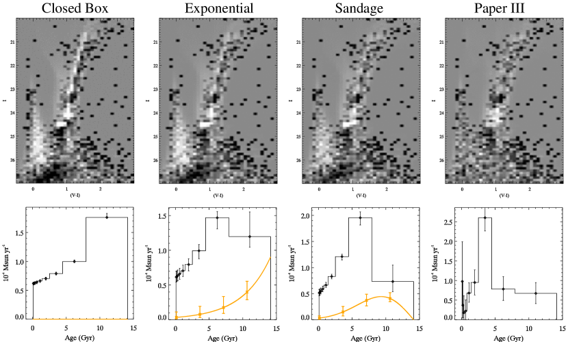
Figure 1: Star formation history and inflow history results using the Padova tracks. The top panel in each column shows the residual CMD on a range of $\pm 3\sigma$ where positive (white) residuals indicate an excess of model stars. The bottom panel in each column shows the star formation history as the upper line and inflow history (scaled by a factor of 0.1 and integrated over the total field area) as the lower line. From left to right, the columns correspond to the closed box, exponential inflow, and Sandage inflow models, respectively. The last column shows the results from Paper III, for which age and metallicity were free parameters.

We tested several different inflow/outflow scenarios using both sets of stellar tracks. In general, they give similar results, so we only show those of the Padova tracks. In the text, we describe any significant differences, since they can help us gauge the systematic errors due to the tracks themselves. The top row in Figs. 1 – 2 shows the residual CMD of a particular scenario on a scale where white and black correspond, respectively, to an excess and deficit of model stars at the $3\sigma$ level. The bottom row in these figures shows the best-fitting SFH as the upper line and inflow history (IFH) divided by 10 as the lower line. The IFH is integrated over the total field area. The last column in these figures gives the result of Paper III, in which age and metallicity were free parameters. Tables 2 and 4 give the the fit quality ($Q$), reduced $\chi^{2}$ ($\chi_{\nu}^{2}$), number of degrees of freedom ($\nu$), and mean distance modulus and extinction with their respective $1\sigma$ uncertainties. Tables 3 and 5 give the mean star formation and outflow efficiencies and their upper and lower $1\sigma$ uncertainties. The mean values reported in the tables are averages of the acceptable solutions in the distance/extinction grid as explained in §3.

4.1 Closed Box Models

We began by testing the canonical closed box model in which the inflow and outflow rates were identically zero. The system was initially composed entirely of gas. The total mass remained constant throughout its evolution while the gas mass and SFR decreased monotonically with time. The best-fitting closed box model is displayed in the first column of Fig. 1.

There are several significant discrepancies between the model and data CMDs. First, the model predicts too much star formation at ages $\la 1$ Gyr which causes an overabundance of model main sequence (MS) stars on the blue plume at $(V-I)\sim 0.0$. Second, the model has too few stars in a region below the blue plume centred at $(V-I)\sim 0.5$ and $I\sim 26.5$. In the global solutions of Paper III, this region is dominated by stars with ages $\sim 2-8$ Gyr, indicating the closed box model has too little star formation at these ages. Also, the RGB of the model is too blue, indicating a mean metallicity that is too low.

The Teramo model exhibits similar discrepancies, but the RGB appears slightly too wide, possibly indicating an excessively large metallicity spread, and it has too many stars overall. The Teramo model also has too many stars on the blue horizontal branch, which signals that there is too much star formation at the oldest ages. It cannot be due to the metallicity of the oldest bin being too low because it is already close to that of the Paper III solution, which does not show such a discrepancy.

The fit qualities of the closed box solutions are $>20\sigma$ worse than the solutions of Paper III, which had $Q$ values of 6.64 (Padova) and 6.02 (Teramo). This is not surprising since our closed box model has only two free parameters, namely, the star formation efficiency and the total mass. However, as we will see below, the addition of gas inflow and outflow significantly improves the fits with only $2-4$ more free parameters, indicating this region in M33 probably did not evolve as a closed box. Because of the reduced number of free parameters, the confidence intervals of the closed box solutions are significantly smaller than those of the Paper III solutions. This demonstrates that simultaneous CMD and chemical evolution modelling can be used to alleviate the age-metallicity degeneracy inherent in broad-band stellar colors.

4.2 Inflow and Outflow Models

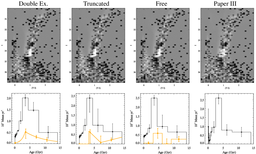
Figure 2: Same as Fig. 1, but the first three columns show the double exponential, truncated, and free inflow models, respectively.

As described in §1, there is evidence that galaxies do not evolve as closed boxes. An exponential inflow rate is one of the simplest and most common forms used in the literature, so it is instructive to see how well it can explain M33’s SFH. Accordingly, we solved for the inflow time-scale and the initial inflow rate. We also included gas outflow by allowing a nonzero outflow efficiency, $w$. The second column in Fig. 1 shows the exponential inflow model for the Padova tracks.

This new model provides a better fit to the data than the closed box model, but it still exhibits some large discrepancies with the data. In fact, these discrepancies are very similar to those of the closed box model, but the magnitude of the residuals has been lessened. There is still too much star formation at ages $\la 1$ Gyr and too little in the range $2-8$ Gyr. The fit quality is $\sim 15\sigma$ worse than the Paper III solutions.

Some numerical simulations of structure formation within the $\Lambda$CDM framework predict that the average mass accretion rates of dark matter haloes are initially small, grow to some maximum, and decline thereafter (e.g., van den Bosch, 2002; Wechsler et al., 2002). With this in mind, we also investigated another function for the IFR which has a delayed maximum, $f_{I}(t)\propto t\ \exp(-t^{2}/2\tau^{2})$, where $\tau$ is the time between when the inflow starts and when it peaks. This function, which we refer to as Sandage inflow, was first used by Sandage (1986) to describe the variation in SFH with galaxy morphology and later explicitly presented by MacArthur et al. (2004). By shifting the bulk of the inflow toward younger ages (i.e., earlier lookback times), it allows for more star formation at correspondingly younger ages. The result is plotted in the third column of Fig. 1. The morphologies of the residuals are similar to the exponential inflow model, but their magnitudes are smaller. The fit quality is $\sim 9\sigma$ worse than the Paper III solutions.

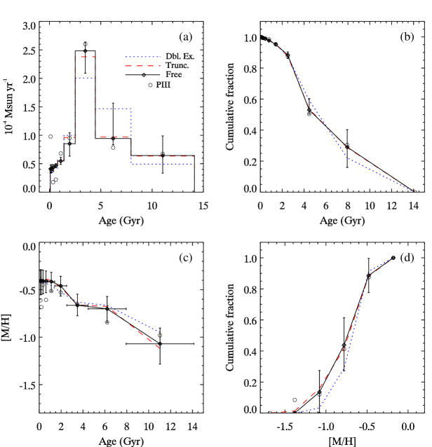
Figure 3: (a) Star formation history, (b) age cumulative distribution function, (c) age-metallicity relation, and (d) metallicity distribution function of the acceptable inflow solutions using the Padova tracks. Each panel shows the double exponential (dotted), truncated (dashed), and free inflow (solid) models and the results from Paper III (open circles). Only the free inflow model errors are shown for the sake of clarity.

The Teramo models show a qualitatively similar behavior – the exponential and Sandage functions do a progressively better job at reproducing the observed CMD, but still do not get the overall age distribution correct. The main drawback of these functions is that the IFR today cannot easily be varied independently of the IFR at intermediate ages ($\sim 2-8$ Gyr). These functions just do not provide enough freedom to describe the true IFH which may not be adequately characterized by just two parameters or a smooth function.

These results led us to try three less restrictive inflow models. The first was a double exponential model described by four parameters: a growing time-scale, a decaying time-scale, a transition time between the growing and decaying modes, and the IFR at the transition time. The second was a truncated model described by four parameters: the initial IFR, the IFR at a model time of 7 Gyr, a truncation time when the inflow ends, and the IFR at the truncation time. In the third model, which we called free inflow, we approximated the true IFH with a discrete function by dividing the entire age range into 4 bins each with a possibly different but constant IFR. We experimented with different binning schemes and settled upon a compromise between the desire to have a reasonable computing time and small error bars (requiring fewer bins) and the competing desire to produce complicated SFHs (requiring more bins). The free inflow model allows discontinuous jumps in the IFR, but these should not be interpreted too literally. This is the same approach that we take in approximating the true SFH with 9 logarithmic bins, each with constant SFR. Internal tests have shown that these inflow functions can reasonably capture broad trends in the true IFH and chemical evolution, especially at ages $\la 7$ Gyr.

The solutions using these three inflow models are displayed in Fig. 2. The free inflow model provides the highest quality fits. However, the double exponential and truncated inflow models are $<1\sigma$ worse and exhibit qualitatively similar results. The discrepancies between model and data exhibited previously with the exponential and Sandage inflow models are almost completely erased. Most of the discrepancies that do remain are similar to those exhibited by the solutions in Paper III, leading us to conclude that they are mostly caused by inaccuracies in the stellar tracks. However, the fit qualities are still $\sim 2-4\sigma$ worse than the Paper III solutions. This difference could arise from the approximations made in producing the chemical evolution models and the uncertainties inherent in the stellar yields. Second, age and metallicity are no longer completely free parameters so errors in the stellar tracks cannot be as easily hidden by arbitrary combinations of age and metallicity. Third, we do not account for a systematic change in the metallicity spread with age. Finally, we have not allowed for an inflow or outflow of stars with other ages and metallicities into the single coherently evolving region we are modelling. This mixing of stars, perhaps caused by gravitational interactions with spiral arms, could artificially increase the spread in the age-metallicity relation and it could mean the stars in this region originated, on average, at another location in M33 (Sellwood & Binney, 2002; Roškar et al., 2008).

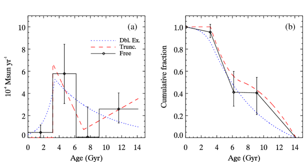
Figure 4: (a) Inflow history and (b) inflow cumulative distribution function of double exponential (dotted line), truncated (dashed line), and free inflow models (solid line) using the Padova tracks. For clarity, only the free inflow model errors are shown.

In Fig. 3, we summarize the distribution of stellar ages and metallicities in the three best inflow models for the Padova tracks. The panels show the (a) SFH, (b) age cumulative distribution function (age CDF), (c) Z AMR, and (d) Z metallicity distribution function (Z MDF) of all stars ever formed. The dotted and dashed lines are, respectively, the double exponential and truncated inflow models. The solid line with diamonds and error bars corresponds to the free inflow model. The open circles are the results from Paper III. Note that only the free inflow model errors are shown for clarity. Additionally, we show the IFH and inflow CDF of these three models in Fig. 4.

In the best three inflow models, $\sim 50-60\%$ of the gas accretion takes place between 3 and 7 Gyr ago. Anything less would produce too few intermediate-age stars. Second, at most $\sim 10\%$ of the gas was accreted in the last 3 Gyr. Any amount in excess of that would lead to a recent SFR that is too high and produce too many young stars on the blue plume MS at $(V-I)\sim 0.0$. Third, the preferred outflow efficiency is $\approx 1\pm 0.5$, which is smaller than the typical values of $\sim 5-10$ estimated for dwarf galaxies in the LG (Lanfranchi & Matteucci, 2004; Carigi et al., 2006). Finally, the results for the SFH, age CDF, AMR, and Z CDF are similar to the Paper III solutions. This lends support to our conclusions in Paper III, and suggests they are not significantly affected by unphysical combinations of age and metallicity.

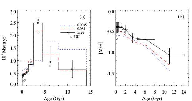
Figure 5: (a) Star formation history and (b) age-metallicity relation using two independently estimated values for M33’s star formation efficiency, $\epsilon=0.0035$ (dotted line) and 0.084 (dashed line; see text for details). The original free inflow model (solid line with diamonds) treated $\epsilon$ as a free parameter, resulting in a best-fitting value of 0.62. Open circles are the results from Paper III. Only the original free inflow model errors are shown for the sake of clarity.

The preferred values for $\epsilon$ tend to be of order $\sim 0.1-1.0$. The resulting gas depletion timescale, $\tau_{g}=\Sigma_{g}/\Sigma_{SFR}$ $\approx 3-10\ \rm Gyr$, is on the low end of the equivalent timescale in dwarf galaxies, which ranges from a few to several tens of Gyr (Taylor & Webster, 2005; Karachentsev & Kaisin, 2007; Calura et al., 2008). An $\epsilon$ value as low as 0.0035 (Heyer et al., 2004) is strongly disfavored because, as Fig. 5 demonstrates, the resulting distributions of stellar age and metallicity are skewed to higher and lower values than the Paper III solution. If, instead, we fix $\epsilon$ to have a higher value, like 0.084, as implied by the local current gas density and SFR in our field, then the age and metallicity distributions are more reasonable. This value of $\epsilon$ is only $1.2\sigma$ larger than the Heyer et al. (2004) value and only $1.1\sigma$ lower than the best-fitting value of 0.62 in the free inflow model. The variation in $\epsilon$ among the best three inflow models indicates the exact parametrization of the IFH can affect it by almost an order of magnitude. Based on the tests in §5, a similar uncertainty in $\epsilon$ arises from various assumptions built into the chemical models, like the stellar yields and the metallicity of the inflowing gas.

By incorporating the chemical evolution equations into the CMD fitting, we can extract more information from the solutions and make more predictions that can be tested against observations. Fig. 6 summarizes some predictions for the three best inflow models. Each figure shows (a) the gas mass averaged over each of the 9 SFH bins, (b) the stellar mass-weighted $\langle$[$\alpha$/Fe]$\rangle$ and $\langle$[Fe/H]$\rangle$ of all stars formed in each SFH bin, (c) the Fe AMR, and (d) the Fe MDF. In panel (b), the horizontal and vertical lines denote $\langle$[$\alpha$/Fe]$\rangle$ and $\langle$[Fe/H]$\rangle$ of all stars ever formed, respectively. The line types are the same as in Fig. 3.

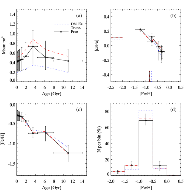
Figure 6: Gas mass and chemical composition in the double exponential (dotted line), truncated (dashed line), and free inflow models (solid line) using the Padova tracks. (a) Evolution of the gas mass surface density, (b) [$\alpha$/Fe] vs. [Fe/H] relation, (c) age-metallicity relation for iron, and (d) metallicity distribution function for iron. Only the free inflow model errors are shown for the sake of clarity. The horizontal and vertical line segments in panel (b) denote, respectively, the mean [$\alpha$/Fe] and [Fe/H] of all stars ever formed.

Because of the presence of gas inflow, the gas mass rises in the early evolutionary stages and reaches a maximum several Gyr later. The gas mass begins to decline as the inflow rate becomes small but star formation and outflow continue. Interestingly, the total mass actually decreases in a few cases when the outflow rate exceeds the inflow rate. The mean [$\alpha$/Fe] of the oldest age bin is $\sim 0.2\pm 0.1$ while that of the youngest bin is $\sim-0.1\pm 0.1$. Because the majority of stellar mass formed within the oldest three age bins, $\langle$[$\alpha$/Fe]$\rangle$ of all stars ever formed is $\sim 0.1$, even though the majority of age bins have $\langle$[$\alpha$/Fe]$\rangle$ $<0.0$. Note that the [$\alpha$/Fe] vs. [Fe/H] relation is not always single-valued, since [$\alpha$/Fe] can increase and [Fe/H] can decrease with time depending on the precise interplay between gas flows, the SFR, and the SN Ia explosion rate (see 7.1).

The Teramo models show an overall similar history as the Padova models, with $\sim 50\%$ of the total inflow taking place in the last 7 Gyr and $\la 5\%$ in the last 3 Gyr. However, the inflow hiatus present in the Padova free inflow model between $\sim 6$ and 9 Gyr is not present in the Teramo model. The mean [$\alpha$/Fe] is also similar between the two sets of tracks. The Teramo models predict gas masses smaller by a factor of $\sim 2$ and metallicities $\sim 0.2$ dex higher at all ages. This metallicity difference is somewhat larger here than in Paper III. We believe this is mostly due to the metallicity of the 6.2 Gyr age bin in the Teramo solution now being $\sim 0.3$ dex larger than it is in Paper III. The overall faster enrichment of the Teramo solutions compared to the Padova solutions requires higher fitted values of $\epsilon$. In a couple of the inflow models, $\epsilon$ reaches its upper limit of 10. We repeated these fits with an upper limit of 100 and the resulting fit qualities were improved by $\sim 1-2\sigma$, but the details of the SFH, IFH, and chemical evolution were not significantly different.

5 Varying the Model Parameters

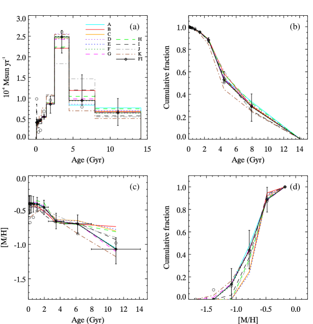
Figure 7: Effects of varying the model parameters on the star formation history and age-metallicity relation using the Padova tracks. The solid line with diamonds is the original free inflow model and the other lines are tests A through K (see text for details). Open circles are the results from Paper III. Only the original free inflow model errors are shown for the sake of clarity. The panels are identical to Fig.  3.

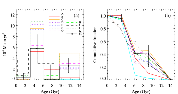
Figure 8: Effects of varying the model parameters on the inflow history using the Padova tracks. The solid line with diamonds is the original free inflow model and the other lines are tests A through K (see text for details). Only the original free inflow model errors are shown for the sake of clarity. The panels are identical to Fig. 4.

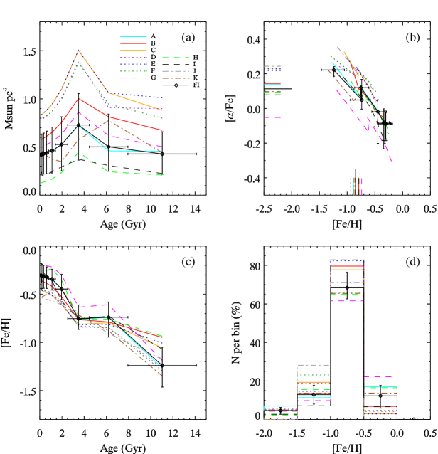
Figure 9: Effects of varying the model parameters on the gas mass and chemical composition using the Padova tracks. The solid line with diamonds is the original free inflow model and the other lines are tests A through K (see text for details). Only the original free inflow model errors are shown for the sake of clarity. The panels are identical to Fig. 6.

There were several parameters in our chemical models which we fixed to match observations or be consistent with previous studies. These parameters included the initial gas mass, initial chemical composition, composition of the inflowing gas, the KS relation exponent, and the stellar yields. To estimate their effects on our results, we varied each of these parameters and repeated the free inflow fit. This resulted in several new models which we refer to as A through K and which had the following parameter changes: (A) an initial unenriched gas reservoir with $\Sigma_{g}(0)=1.0\ M_{\sun}\ \rm pc^{-2}$, (B) the same as A but the gas reservoir was pre-enriched to [Fe/H] $=-1.3$, (C) the inflowing gas was pre-enriched by SNe II to [Fe/H] $=-1.3$, (D) a superposition of A and C, (E) a superposition of B and C, (F) $y_{i}$ was increased by a factor of 2, (G) $y_{i}$ was decreased by a factor of 2, (H) $\kappa=1.4$, and (I) a different binning scheme was used. We also ran two additional tests in which $\epsilon$ was allowed to vary with time: (J) a closed box model with an initial metallicity of [Fe/H] $=-1.3$ and (K) a free inflow model with a constant IFR (i.e., one inflow bin rather than 4). While these tests are by no means exhaustive, they give a rough sense of the potential systematic errors that could be introduced by the assumptions we made in our chemical models.

Figs. 7 – 9 compare the original best-fitting free inflow model (line with diamonds and error bars) to the new models (lines without error bars). The open circles are the results from Paper III. Note that only the original free inflow model errors are shown for clarity.

In general, the new results are not significantly different from the original results and the fit qualities are unchanged to within $\sim 1\sigma$. The SFH, age CDF, MDF, and Z CDF are the least affected by the new parameter values and they remain close to the results of Paper III. More variation occurs in the IFH, inflow CDF, gas mass evolution, and [$\alpha$/Fe] vs. [Fe/H] relation. The IFR and gas mass in any age bin can show variations up to a factor of $\sim 2$. The presence of an initial gas reservoir, as in models A, B, D, and E, decreases the amount of inflow required in the oldest bin because otherwise the resulting SFR would be too high. This means that, all else being equal, the fraction of total inflow occurring at younger ages ($\la 7$ Gyr) in the original models is a lower limit. Increasing [Fe/H] of the initial gas reservoir only increases $\langle$[Fe/H]$\rangle$ and $\langle$[$\alpha$/Fe]$\rangle$ of the oldest age bin. All else being equal, increasing [Fe/H] of the inflowing gas shifts $\langle$[$\alpha$/Fe]$\rangle$ of all age bins upward $\sim 0.1$ dex and shifts the initial and final $\langle$[Fe/H]$\rangle$ upward and downward by $\sim 0.2$ dex, respectively. Models C – F have some of the largest IFRs and gas mass densities. In model F, a larger IFR of primordial gas is needed to balance the increased stellar yields. When the inflowing gas is not primordial, as in models C – E, more of it is required to counteract the ISM enrichment due to stellar nucleosynthesis.

One of the largest sources of uncertainty in chemical evolution models is the stellar yields. Changing the instantaneous yields, $y_{i}$, by a factor of 2, as in models F and G, shifts the [$\alpha$/Fe] vs. [Fe/H] relation vertically by $\sim 0.1-0.2$ dex with only a small change to the relation’s tilt. Increasing or decreasing the delayed yields, $y_{i,d}$, has the same effect on the [$\alpha$/Fe] vs. [Fe/H] relation as decreasing or increasing, respectively, the instantaneous yields. This fact arises because the $\alpha$-elements contribute the majority of $y_{i}$ while iron contributes the majority of $y_{i,d}$. Decreasing $y_{i}$ or increasing $y_{i,d}$ appear to be the only ways to significantly move the entire [$\alpha$/Fe] vs. [Fe/H] relation down relative to the original model.

To demonstrate the binning effects on the results, Model I has a different binning scheme from the original free inflow solution. Instead of 4 bins, Model I uses the same 9 logarithmically spaced bins as the SFH. This model is within $1\sigma$ of the original free inflow model and has a similar inflow history and chemical evolution to within the errors. The two most important differences are that, first, the inflow hiatus appearing in the original model is no longer present. This hiatus was possible in the original model, and not the new one, because of the overlap between the 2nd oldest SFH bin and 3rd oldest IFH bin. Second, the new binning scheme allows a large inflow burst in the youngest two bins ($\sim 80-250$ Myr) amounting to $\sim 10\%$ of the total inflow. During this burst, the IFR increases by a factor $>1000$ over the previous two bins. This burst occurs in order to reproduce the apparent SFR burst in the youngest bin seen in the Paper III solution. As the tests and discussion in Paper III bear out, the reality of such a SFH burst is highly suspect because the SFR amplitudes in the youngest couple of age bins are susceptible to low number statistics.

In all the preceding results, we have attributed variations in SFR primarily to variations in IFR because the star formation efficiency, $\epsilon$, was constant with time. A natural question to ask is, can the SFR variations be due, instead, to variations in $\epsilon$? Allowing $\epsilon$ to vary weakens the link between SFH and IFH, but does not completely decouple them because $\epsilon$ and the IFR have opposite effects on the ISM metallicity. A sudden increase in the IFR dilutes the metals in the ISM, decreasing the enrichment rate, whereas a sudden increase in $\epsilon$ increases the SFR and, hence, enrichment rate. Phenomena like gravitational perturbations and stellar feedback could potentially change $\epsilon$, which may more generally evolve according to local gas phase properties like temperature, density, pressure, chemical composition, molecular fraction, and interstellar radiation field strength (e.g. Elmegreen, 1993; Sommer-Larsen et al., 2003; Schaye, 2004; Schaye & Dalla Vecchia, 2008; Robertson & Kravtsov, 2008).

Models J and K respectively demonstrate that a closed box or constant IFR model provide an acceptable fit to the CMD if we allow $\epsilon$ to vary with time. However, the amount of variation required (an r.m.s. deviation over time $\sim 0.5$ dex) may be larger than the intrinsic scatter in the KS relation of other spirals given the vagaries of H$\alpha$ extinction corrections and the $\rm H_{2}$-CO conversion factor (Kennicutt, 1998; Wong & Blitz, 2002; Komugi et al., 2005; Kennicutt et. al., 2007; Boissier et. al., 2007). Also, the initial metallicity in model J must be non-zero, otherwise there are too many metal-poor stars. This model does a poor job of reproducing the observed present-day gas surface density of $\sim 0.8\ M_{\sun}\ \rm pc^{-2}$ (see §6). The gas density in model J decreases from about 3 to 2.3 $M_{\sun}\ \rm pc^{-2}$ for the Padova tracks and from about 2.2 to 1.5 $M_{\sun}\ \rm pc^{-2}$ for the Teramo tracks. Hence, this quantity is above the range plotted in panel (a) of Fig. 9. In model K, the AMR decreases over the last 2 Gyr because gas inflow continues while very few stars form. Model K also has more gas inflow ($\sim 20\%$) occurring in the last 3 Gyr than the original free inflow model ($<10\%$).

6 Comparison to Observations in M33

Next, we will examine in further detail the predictions of the original free inflow solutions, since they provide the best fits. The Padova solutions have a present-day gas mass of $\sim 0.4\ \pm\ 0.2\ M_{\sun}\ {\rm pc^{-2}}$. From the difference between the Padova and Teramo solutions, we estimate a systematic error of a factor of $\sim 2$ due to uncertainties in the stellar tracks. The projected mean HI column density in this field is $\sim 1.1\ M_{\sun}\ {\rm pc^{-2}}$, as measured from a mosaic constructed from Very Large Array and Green Bank Telescope observations (D. Thilker, private communication). If we correct for a disc inclination of $56\degr$ and for a helium abundance one-third that of hydrogen, then this becomes $\sim 0.8\ M_{\sun}\ {\rm pc^{-2}}$. The true inclination of the HI disc at this location is somewhat uncertain because of the well-known warp at large radii (Corbelli & Schneider, 1997). A change of $\pm 10\degr$ in the inclination would change the surface density by approximately $\pm\ 0.2\ M_{\sun}\ {\rm pc^{-2}}$. For comparison, the azimuthally-averaged HI column density at this radius in M33 is $\sim 3\ \rm M_{\sun}\ pc^{-2}$ (Corbelli & Schneider, 1997; Corbelli, 2003).

The present-day SFR provides another useful check on our results. Using GALEX near-UV and far-UV images of M33, Boissier et al. (2007; private communication) computed the UV surface brightness in our field and then converted that to a SFR using the relation in Kennicutt (1998), which is a slightly modified version of the one first presented in Madau et al. (1998). The infrared data used to estimate extinction was of poor quality this far out in M33, so the SFR could only be constrained to the range $\sim(0.6-0.9)\times 10^{-4}\ M_{\sun}\ {\rm yr^{-1}}$, where the lower limit corresponds to zero extinction and the upper limit corresponds to an extinction of $A_{FUV}=0.49$. The azimuthally-averaged UV SFR at this radius lies at the lower limit. The chief sources of uncertainty in these limits are the UV flux-SFR calibration, which was based on theoretical isochrone and spectral libraries, and the assumption of a Salpeter IMF. According to Madau et al. (1998), adopting a Scalo IMF (Scalo, 1986), which is more similar to the IMF we have used, the resulting SFR would be $\sim 50\%$ smaller. Therefore, the range above becomes $\sim(0.3-0.5)\times 10^{-4}\ M_{\sun}\ {\rm yr^{-1}}$, which is in good agreement with our predictions of $\sim 0.4$ and $0.3\times 10^{-4}\ M_{\sun}\ {\rm yr^{-1}}$ for the Padova and Teramo free inflow solutions, respectively.

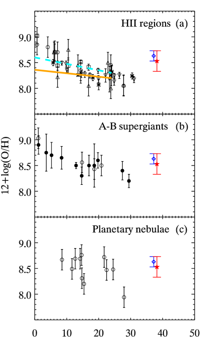
Figure 10: Oxygen abundances as measured in (a) H ii regions, (b) A-B supergiant stars, and (c) PNe. The solid and dashed lines in panel (a) come from Rosolowsky & Simon (2008) and Viironen et al. (2007), respectively. In all three panels, the star and diamond are, respectively, the Padova and Teramo free inflow model predictions for the present day oxygen abundance. Their abscissa values are offset from each other for clarity.

Another important check comes from oxygen abundances in M33. Magrini et al. (2007) compiled an extensive catalog of previously measured abundances in H ii regions, type A-B supergiant stars, and planetary nebulae (PNe). This catalog is plotted in Fig. 10 with the predictions of the Padova and Teramo free inflow models for the present-day oxygen abundance (star and diamond, respectively), whose abscissa values are offset from each other for clarity. The H ii regions and supergiants probe the present-day ISM abundance whereas the PNe probe the ISM abundance at older ages. The masses and lifetimes of the PNe progenitors are not known with great certainty. The sample of Magrini et al. covers only the brightest two magnitudes of the PNe luminosity function, so it could be biased toward the high end of the progenitor mass range. Therefore, the progenitors probably had MS lifetimes less than a few Gyr.

Most of the H ii region abundances in the Magrini et al. compilation were made from direct $T_{e}$ measurements, generally considered the most reliable kind. Eight objects have at least two independent measurements and three of those objects have three independent measurements. We have also added the recent gradient derived by Viironen et al. (2007) (dashed line) for $\sim 60$ H ii regions based on the $\rm log(H\alpha/$[S ii]$\lambda\lambda 6717+6731)$ vs. $\rm log(H\alpha/$[N ii]$\lambda 6583)$ diagnostic diagram. Recently, Rosolowsky & Simon (2008) reported oxygen abundances of 61 H ii regions in the southwest region of M33 derived from the temperature sensitive emission line [O iii] $\lambda 4363$ Å. They found a shallow gradient which we show as the solid line in Fig. 10.

Our results are more consistent with an overall shallow gradient or a flattening in the gradient at large radii (Magrini et al., 2007) than they are with a constant gradient over M33’s entire disc. However, even if the gradient was flat beyond $R_{dp}\sim 30\arcmin$, our results would be several tenths of a dex higher than expected from the data in Fig. 10. The magnitude of this discrepancy is comparable to the random and systematic uncertainties in our results, so it may not be statistically significant. Moreover, Rosolowsky & Simon (2008) noted a scatter of 0.11 dex in their sample unattributable to measurement errors, possibly indicating chemical inhomogeneities in M33’s ISM. This fact also highlights the importance of using large samples of objects at many position angles within the disc. More importantly, the data in Fig. 10 have their own systematic uncertainties. For example, the abundances of H ii regions tend to be lower than supergiants and PNe by $\sim 0.2$ dex. This offset could indicate a problem in how the temperature and ionization structures of H ii regions are treated (e.g., García-Rojas & Esteban, 2007; Esteban et al., 2004; Kennicutt et al., 2003, and references therein), but larger samples need to be compared before the nature of this discrepancy can be fully understood.

7 Discussion

7.1 Comparison to Models of the Solar Vicinity and Magellanic Clouds

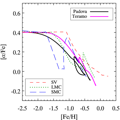
Figure 11: Comparing the [$\alpha$/Fe] vs. [Fe/H] relation for M33, the SV, LMC, and SMC. The solid lines are the free inflow solutions while the other lines are the chemical models in PT95 and PT98.

In Fig. 11, we compare the [$\alpha$/Fe] vs. [Fe/H] relation in this region of M33 to that of the SV, LMC, and SMC derived in PT95 and PT98. The models for these other three systems have been cited often in the literature because of their simplicity and ability to reproduce observations fairly well. The solid lines show the free inflow solutions using the Padova and Teramo tracks without being averaged over each SFH bin. Viewing the relation in this manner facilitates comparison with the other systems and can lead to greater physical insight, as long as we remember that the overall shape is most robust. This last fact can be appreciated from the overall similarity of the acceptable inflow solutions in Fig.  6.

Fig. 11 reveals that M33’s [$\alpha$/Fe] vs. [Fe/H] relation is generally similar to the other systems. Because we have used almost identical chemical evolution equations and identical stellar yields as PT95 and PT98, our models show a similar overall behavior in response to gas flows. The discontinuities in the relation for each system can be traced back to the interplay between the SFR, IFR, and the delayed injection of iron into the ISM from SNe Ia. Therefore, the differences between the relations arise primarily from differences in the SFH and IFH.

In the IRA, the abundance ratio of any two elements is a constant determined by the ratio of their nucleosynthetic yields. Thus, the initial $[\alpha/{\rm Fe}]$ ratio is ${\rm log}(y_{\alpha}/y_{\rm Fe})-{\rm log}(X_{\alpha}/X_{\rm Fe})_{\sun}\approx~{}0.4$. After 1.3 Gyr have elapsed, the DPA begins operating as the first SN Ia inject iron into the ISM and produce the first downturn, or “knee”, in the relation. The [Fe/H] location of this knee is dependent on the SFR, which, in turn, depends on the IFR and outflow rate. The SFR was on average higher in the SV than in the other systems, so it experienced a faster enrichment and the knee occurs at a higher metallicity.

The large loop in the Padova model results from three successive steps: a sudden large increase in the IFR at an age $\sim 6$ Gyr which dilutes metals in the ISM (see the IFH in Fig. 4a), a corresponding increase in the SFR which raises [$\alpha$/Fe], and the subsequent drop in [$\alpha$/Fe] 1.3 Gyr later due to SN Ia. The Teramo model experiences a much smaller loop because it does not have as large an increase in the IFR at 6 Gyr.

7.2 Implications for the Formation of the MW’s Halo

The $\Lambda$CDM hierarchical picture of galaxy formation predicts that dark matter haloes are built up from the accretion/merging of smaller subhaloes similar to the protogalactic fragments proposed by Searle & Zinn (1978). This picture can be tested by comparing the chemical composition of the MW’s stellar halo field population to such subhaloes or their possible present-day analogs, such as the MW’s dSph satellites. As reviewed in detail by Geisler et al. (2007) and references therein, the MW’s field halo population is chemically distinct from these other systems, indicating that the former was not built up from the latter. In particular, the present-day dSphs and other LG galaxies are characterized by [$\alpha$/Fe] ratios lower than most of the MW’s halo, especially at [Fe/H] $\ga-2$. This is commonly interpreted to mean that the SFR in the dSphs was lower and, therefore, their chemical enrichment was too slow to reach the halo’s metallicity with a high [$\alpha$/Fe] before SNe Ia contributed significant amounts of iron.

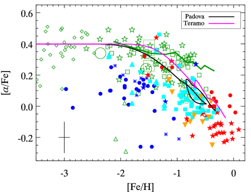
Figure 12: Comparing the [$\alpha$/Fe] vs. [Fe/H] relation in one location in M33’s outskirts to spectroscopic abundance ratios of individual stars in various LG systems. The data were compiled from the literature and presented in Geisler et al. (2007), to which we refer the reader for more details. The systems shown are the MW halo (green open points and green line), low-mass dSphs (blue filled circles, stars, and asterisks), Sagittarius dSph (red filled circles and stars), LMC (cyan filled squares and upward pointing triangles) and dIrrs (orange filled downward pointing triangles). The Padova and Teramo free inflow models are black and magenta lines, respectively. The error bars in the lower left corner represent typical random measurement uncertainties.

It is interesting to compare our results for M33’s outer disc to the spectroscopic measurements in other LG systems. Such an exercise places our results into the context of the LG as a whole and could have some implications for the formation of the MW’s halo. To that end, in Fig. 12, we summarize the high-resolution spectroscopic measurements of [$\alpha$/Fe] and [Fe/H] in these systems. This figure is reproduced from Geisler et al. (2007) except that we have added the Padova and Teramo free inflow solutions as the black and magenta lines  . The green line represents the halo’s dissipative collapse component while the green open stars represent the halo’s accretion component, as defined by Gratton et al. (2003) based on orbital kinematics. These authors postulated the dissipative component formed during the collapse of the MW’s gaseous halo, as earlier outlined by Eggen et al. (1962), and the accretion component originated in the accreted subhaloes.

The green open diamonds at [Fe/H] $\sim-3$ represent extremely metal-poor halo giants analysed by Cayrel et al. (2004), for which no separation into kinematic components has been made. All other green open points represent samples of MW halo stars selected for their unusual orbital properties and which therefore are additional candidates for originating in chaotically accreted subhaloes. The other systems represented in Fig. 12 are low-mass dSph satellites of the MW (blue filled circles, stars, and asterisks), Sagittarius dSph (red filled circles and stars), LMC (cyan filled squares and upward pointing triangles), and several dIrrs (orange filled downward pointing triangles). Typical random measurement uncertainties are indicated in the bottom left corner. We refer the reader to Geisler et al. (2007) for a more detailed explanation and for a list of all the references for the data.

Based on our results, if we could obtain high resolution spectroscopic abundances for the location we have studied in M33, we would expect most of its stars to lie near $\langle$[$\alpha$/Fe]$\rangle\sim 0.1$ and $\langle$[Fe/H]$\rangle\sim-0.7$. Of all the systems presented in Fig. 12, this region of parameter space is most similar to the LMC. We also note that M33 resembles the MW’s halo more than the low-mass dSphs. The plateau at [Fe/H] $\la-2.0$ was built into the models via the chemical yields (see §7.1), but the key fact is that M33 maintains a higher [$\alpha$/Fe] ratio at a given [Fe/H] relative to the low-mass dSphs. The agreement between M33 and the MW’s halo becomes progressively worse at [Fe/H] $\ga-2$. However, M33’s relation overlaps with some of the candidate accretion stars suggesting they could have originated in a system whose SFH, AMR, and IFH were similar to M33’s outer disc, though not necessarily a spiral galaxy like M33. This is consistent with the suggestion of Geisler et al. (2007) that some of the accreted MW halo stars originated in high mass dwarf systems.

Although we have little information on M33’s inner disc evolution, the presence of a metallicity gradient (Magrini et al., 2007) and a wide variety of ages inferred from CMDs (Sarajedini et al., 2000) hint at an extended SFH with a faster enrichment taking place there. Therefore, we hypothesize that the knee in the [$\alpha$/Fe] vs. [Fe/H] relation in M33’s inner disc occurs at a higher metallicity than in the outer disc. This brings us to another key point, that candidate accretion halo stars with different [$\alpha$/Fe] but the same [Fe/H] did not necessarily originate in different objects. In other words, the $\alpha$-element and iron abundances alone do not necessarily provide enough information to tag individual halo stars to unique progenitors (Freeman & Bland-Hawthorn, 2002). This is because the inner regions of a protogalactic fragment could have become enriched with metals faster than the outer regions. Therefore, the candidate accretion stars that we observe today with low and high [$\alpha$/Fe] could have originated in the outer and inner regions of the fragment, respectively.

How realistic is such a scenario? How much time would have been necessary and available for this hypothetical fragment to attain the range of [Fe/H] and [$\alpha$/Fe] observed today in the MW halo’s accreted stars? Our results indicate M33’s outskirts took $\sim 4$ Gyr to reach [Fe/H] $\ga-1.0$ and [$\alpha$/Fe] $\sim 0.1$. Zentner & Bullock (2003) used a semi-analytic model to examine the survival of orbiting subhaloes in the MW’s potential. They found that for a typical subhalo orbit, the survival time after entering the MW’s halo ranged from 3 to over 8 Gyr, depending on the subhalo’s mass and concentration relative to the MW’s. Any time spent outside the MW halo prior to accretion would only relax the necessary post-accretion survival time. Thus, it seems entirely plausible that this hypothetical fragment could have had enough time to develop a population gradient before disruption.

Present-day population gradients have been found in most of the dSphs (e.g., Harbeck et al., 2001; Winnick, 2003; Tolstoy et al., 2004; Koch et al., 2006; Stetson et al., 1998; Bellazzini et al., 2005; Battaglia et al., 2006; Faria et al., 2007; Komiyama et al., 2007; McConnachie et al., 2007), in the Sagittarius stream (Bellazzini et al., 2006; Chou et al., 2007), NGC 6822 (de Blok & Walter, 2006), and in M33 (Rowe et al., 2005, Paper II, Paper III). In most cases, the inner regions of the galaxies are more metal rich and/or older than the outer regions. In another recent study, Bernard et al. (2008) found that RR Lyrae stars in the central region of Tucana were more metal-rich than in the outer region, suggesting a metallicity gradient was already present in the first few Gyr of that galaxy’s history.

The evolution of metallicity gradients in disc galaxies is a matter of some debate, with some studies predicting the gradient to increase with time and others predicting the opposite (Magrini et al., 2007, and references therein). The evolutionary model of M33 presented in Magrini et al. (2007) predicts the metallicity gradient to have been steeper in the past. Measurements of the spatially resolved SFH and AMR of these low mass galaxies could help us understand if they can develop chemical gradients in the first few Gyr of their lives or if such gradients were present in the gas from which they formed.

8 Conclusions

In the framework of a simple chemical evolution scenario which adopts instantaneous and delayed recycling for the nucleosynthetic products of Type II and Ia SNe, we have modelled the observed CMD in one location in M33’s outskirts. In this scenario, interstellar gas forms stars at a rate modulated by the KS relation and gas outflow occurs at a rate proportional to the SFR. Compared to the common CMD fitting method of allowing age and metallicity to be free parameters, this scenario yields a more physically self-consistent SFH with fewer free parameters and makes more predictions that can be tested with independent observations. Moreover, this method puts broad constraints on the role of gas flows and extends the method of chemical fingerprinting to stellar systems, like M33, that are beyond the reach of current high resolution spectrographs.

The precise details of our results depend on which stellar evolutionary tracks are used, Padova or Teramo. Nevertheless, the broad trends appear to be robust. We found that, when the star formation efficiency, $\epsilon$, is constant, the canonical closed box model fails to reproduce the observed distribution of stars in the CMD. Models with an exponentially declining IFR from 14.1 Gyr ago exhibit similar discrepancies, but to a lesser magnitude. Instead, the inflow models which best reproduce the observed CMD have a significant fraction ($\ga 50\%$) of gas inflow taking place in the last 7 Gyr and a smaller fraction ($<10\%$) taking place within the last 3 Gyr. This leads to a SFH in overall agreement with what we found in Paper III, and suggests the traditional method of synthetic CMD fitting can be physically self-consistent.

Allowing $\epsilon$ to vary with time, as might be expected if the star formation time-scale depends on local ISM properties, significantly improves the closed box model if the initial metallicity is [Fe/H] $\sim-1.3$, but the resulting present-day gas mass surface density is too high compared to the observed value. A model with a varying $\epsilon$ and constant, non-zero IFR reproduces the CMD and gas mass about as well as the best constant $\epsilon$ models. In this case, more inflow can take place in the last 3 Gyr, but there is still a significant fraction ($\sim 50\%$) of inflow occurring over the last 7 Gyr. The amount of variation in $\epsilon$ required by these models, however, could be larger than the intrinsic scatter in the KS relation of other galaxies.

We also examined the [$\alpha$/Fe] vs. [Fe/H] relation, a key diagnostic of the evolutionary history of stellar systems. Like the MW’s dwarf satellites, the bulk of stars at this location in M33’s outskirts have [$\alpha$/Fe] ratios lower than the MW’s halo field. Stars formed over 8 Gyr ago have $\langle$[$\alpha$/Fe]$\rangle$ $\sim 0.2\pm 0.1$ and stars forming today have $\langle$[$\alpha$/Fe]$\rangle$ $\sim-0.1\pm 0.1$. The mean [$\alpha$/Fe] ratio of all stars ever formed at this location in M33 was found to be $\sim 0.1\pm 0.1$. From the tests we have conducted, we estimate that the systematic errors of these values are $\sim\pm 0.2$ dex, comparable to that of some high resolution spectroscopic measurements of other systems (e.g. Monaco et al., 2005; Geisler et al., 2007).

Our results paint a picture in which M33’s outer disc formed from the protracted inflow of gas over several Gyr with at least half of the total inflow occurring since $z\sim 1$, but relatively little since $z\sim 0.25$. All the acceptable inflow models have a similar IFR $\sim 2\times 10^{-4}\ \rm M_{\sun}\ yr^{-1}\ kpc^{-2}$ averaged over the lifetime of the Universe. This estimate is uncertain by at least a factor of 2 and the IFR could have intrinsic variations of a factor of $\sim 3$ when averaged over 2 $-$ 3 Gyr time-scales. Nevertheless, it still gives a rough indication of the mean gas IFR that could occur in the outskirts of low mass spiral galaxies.

A useful baseline for comparison is the lifetime average IFR in the SV, predicted by Colavitti et al. (2008) to be $\sim 4\times 10^{-3}\ \rm\ M_{\sun}\ yr^{-1}\ kpc^{-2}$. This estimate comes from several chemical evolution models which adopt different shapes for the IFH and which reproduce many local observables, like the abundances of various elements, MDF of long-lived stars, and present-day gas fraction, total mass density, SFR, IFR, and SN rate. That the mean IFR in the SV has been higher than in M33’s outer disc is not surprising since the MW is more massive than M33 and the SV is at a much smaller radius (in terms of disc scale lengths) than the M33 field we have studied.

Sommer-Larsen et al. (2003) ran an N-body cosmological simulation and selected 12 dark matter haloes for more detailed simulations which included baryons. Two Milky Way-type spirals, S1 and S2, that resulted from the simulations experienced gas accretion at a mean rate of $\sim 10^{-3}\ M_{\sun}\rm\ yr^{-1}\ kpc^{-2}$ at radii of $6-7$ disc scale lengths. This rate is about 5 times larger than the mean IFR we have found at a similar location in M33’s outer disc, but S1 and S2 were about 5 times more massive than M33. The total disc averaged accretion rates of the least massive simulated galaxies, with rotation velocities comparable to M33’s, were $\sim 15-35\%$ smaller than those of S1 and S2 at $z=0$. Therefore, if the outer disc accretion rate scales with a galaxy’s rotation velocity in the same way as the total disc averaged rate, and if this scaling holds for all redshifts, then our results are consistent with the simulations of Sommer-Larsen et al. (2003).

What is the source and nature of the gas inflow? If it occurs in the disc plane, it could be caused by spiral density waves, viscosity in the disc gas, or gas with lower angular momentum falling onto the disc at larger radii and flowing toward M33’s nucleus (Lacey & Fall, 1985; Lin & Pringle, 1987; Bertin & Lin, 1996; Portinari & Chiosi, 2000; Roškar et al., 2008). Gas flowing from above the disc plane could come from the condensation of a hot halo corona as described in §1. However, such a process is expected to be more efficient in a massive spiral like the MW than in a late-type spiral like M33 (Dekel & Birnboim, 2006).

The condensed clouds predicted by numerical simulations to fall onto a disc galaxy have properties similar to the MW’s HVC population (Peek et al., 2008). Recent surveys of HI emission around M31 and M33 have revealed an analogous HVC population around these galaxies (Thilker et al., 2004; Braun & Thilker, 2004; Grossi et al., 2008). Thilker et al. (2004) detected 20 clouds within 50 kpc of M31’s disc and the maps presented by Grossi et al. (2008) show many within $\sim 20$ kpc of M33 with an inferred total mass $\geq 5\times 10^{7}\ M_{\sun}$. The M31/33 clouds appear to have a mean mass $\sim 10^{5}\ M_{\sun}$ and size $\sim 1$ kpc (Westmeier et al., 2005; Grossi et al., 2008). The lifetime integrated inflow mass of $\sim 10^{6}\ M_{\sun}$ in the M33 region we have studied requires the accretion of $\sim 10$ such clouds. Extrapolation to M33’s entire disc is risky given how little we know about its evolution and the population of clouds around M33. In addition to condensed halo gas, the clouds could also be low-mass dark matter subhaloes that never formed stars or the tidal debris from recent mergers and interactions (Thilker et al., 2004; Grossi et al., 2008). In the future, we plan to apply the techniques presented in this paper to other regions of M33 and other galaxies. This approach can provide insights on the origin and amount of accreted gas and coupling (or lack thereof) between the baryonic and dark matter accretion histories of these systems.

References

- Abadi et al. (2003) Abadi M. G., Navarro J. F., Steinmetz M., Eke V. R., 2003, ApJ, 597, 21
- Adelberger et al. (2003) Adelberger K. L., Steidel C. C., Shapley A. E., Pettini M., 2003, ApJ, 584, 45
- Anders & Grevesse (1989) Anders E., Grevesse N., 1989, Geochim. Cosmochim. Acta, 53, 197
- Aparicio & Gallart (2004) Aparicio A., Gallart C., 2004, AJ, 128, 1465
- Aparicio et al. (1997) Aparicio A., Gallart C., Bertelli G., 1997, AJ, 114, 680
- Barker et al. (2007a) Barker M. K., Sarajedini A., Geisler D., Harding P., Schommer R., 2007a, AJ, 133, 1125 (Paper II)
- Barker et al. (2007b) Barker M. K., Sarajedini A., Geisler D., Harding P., Schommer R., 2007b, AJ, 133, 1138 (Paper III)
- Battaglia et al. (2006) Battaglia G., Tolstoy E., Helmi A., Irwin M. J., Letarte B., Jablonka P., Hill V., Venn K. A., Shetrone M. D., Arimoto N., Primas F., Kaufer A., Francois P., Szeifert T., Abel T., Sadakane K., 2006, A&A, 459, 423
- Bellazzini et al. (2005) Bellazzini M., Gennari N., Ferraro F. R., 2005, MNRAS, 360, 185
- Bellazzini et al. (2006) Bellazzini M., Newberg H. J., Correnti M., Ferraro F. R., Monaco L., 2006, A&A, 457, L21
- Bernard et al. (2008) Bernard E. J., Gallart C., Monelli M., Aparicio A., Cassisi S., Skillman E. D., Stetson P. B., Cole A. A., Drozdovsky I., Hidalgo S. L., Mateo M., Tolstoy E., 2008, ApJ, 678, L21
- Bertin & Lin (1996) Bertin G., Lin C. C., 1996, Spiral Structure in Galaxies. MIT Press, Cambridge, MA
- Boissier et al. (2003) Boissier S., Prantzos N., Boselli A., Gavazzi G., 2003, MNRAS, 346, 1215
- Boissier et. al. (2007) Boissier S. et. al., 2007, ApJS, 173, 524
- Bosma (1991) Bosma A., 1991, in Casertano S., Sackett P. D., Briggs F. H., eds, Warped Disks and Inclined Rings around Galaxies. Cambridge Univ. Press, Cambridge, p. 181
- Bournaud et al. (2007) Bournaud F., Jog C. J., Combes F., 2007, A&A, 476, 1179
- Braun & Thilker (2004) Braun R., Thilker D., 2004, in Prada F., Martinez Delgado D., Mahoney T. J., eds, Satellites and Tidal Streams. Astron. Soc. Pac., San Francisco, p. 139
- Calura et al. (2008) Calura F., Lanfranchi G. A., Matteucci F., 2008, A&A, 484, 107
- Carigi et al. (2006) Carigi L., Colín P., Peimbert M., 2006, ApJ, 644, 924
- Carigi et al. (2002) Carigi L., Hernandez X., Gilmore G., 2002, MNRAS, 334, 117
- Cassisi et al. (2004) Cassisi S., Salaris M., Castelli F., Pietrinferni A., 2004, ApJ, 616, 498
- Castelli & Kurucz (2003) Castelli F., Kurucz R. L., 2003, in Piskunov N., Weiss W. W., Gray D. F., eds, IAU Symp. 210, Modelling of Stellar Atmospheres. Astron. Soc. Pac., San Francisco, p. A20
- Cayrel et al. (2004) Cayrel R., Depagne E., Spite M., Hill V., Spite F., François P., Plez B., Beers T., Primas F., Andersen J., Barbuy B., Bonifacio P., Molaro P., Nordström B., 2004, A&A, 416, 1117
- Charbonneau (1995) Charbonneau P., 1995, ApJS, 101, 309
- Chiappini et al. (2001) Chiappini C., Matteucci F., Romano D., 2001, ApJ, 554, 1044
- Chou et al. (2007) Chou M.-Y., Majewski S. R., Cunha K., Smith V. V., Patterson R. J., Martínez-Delgado D., Law D. R., Crane J. D., Muñoz R. R., Garcia López R., Geisler D., Skrutskie M. F., 2007, ApJ, 670, 346
- Colavitti et al. (2008) Colavitti E., Matteucci F., Murante G., 2008, preprint (astro-ph/0802.1847)
- Corbelli (2003) Corbelli E., 2003, MNRAS, 342, 199
- Corbelli & Schneider (1997) Corbelli E., Schneider S. E., 1997, ApJ, 479, 244
- de Blok & Walter (2006) de Blok W. J. G., Walter F., 2006, AJ, 131, 343
- Dekel & Birnboim (2006) Dekel A., Birnboim Y., 2006, MNRAS, 368, 2
- Dolphin (2002) Dolphin A. E., 2002, MNRAS, 332, 91
- Dolphin et al. (2005) Dolphin A. E., Weisz D. R., Skillman E. D., Holtzman J. A., 2005, preprint (astro-ph/0506430)
- Dotter et al. (2007) Dotter A., Chaboyer B., Ferguson J. W., Lee H.-c., Worthey G., Jevremović D., Baron E., 2007, ApJ, 666, 403
- Dotter et al. (2007) Dotter A., Chaboyer B., Jevremović D., Baron E., Ferguson J. W., Sarajedini A., Anderson J., 2007, AJ, 134, 376
- Edge & Stewart (1991) Edge A. C., Stewart G. C., 1991, MNRAS, 252, 414
- Eggen et al. (1962) Eggen O. J., Lynden-Bell D., Sandage A. R., 1962, ApJ, 136, 748
- Elmegreen (1993) Elmegreen B. G., 1993, ApJ, 411, 170
- Erb et al. (2006) Erb D. K., Shapley A. E., Pettini M., Steidel C. C., Reddy N. A., Adelberger K. L., 2006, ApJ, 644, 813
- Esteban et al. (2004) Esteban C., Peimbert M., García-Rojas J., Ruiz M. T., Peimbert A., Rodríguez M., 2004, MNRAS, 355, 229
- Faria et al. (2007) Faria D., Feltzing S., Lundström I., Gilmore G., Wahlgren G. M., Ardeberg A., Linde P., 2007, A&A, 465, 357
- Fenner et al. (2006) Fenner Y., Gibson B. K., Gallino R., Lugaro M., 2006, ApJ, 646, 184
- Ferguson et al. (2007) Ferguson A., Irwin M., Chapman S., Ibata R., Lewis G., Tanvir N., 2007, in Island Universes: Structure and Evolution of Disk Galaxies, ed. R. S. de Jong (Dordrecht: Springer), p. 239
- Fox et al. (2007) Fox A. J., Ledoux C., Petitjean P., Srianand R., 2007, A&A, 473, 791
- Fraternali & Binney (2008) Fraternali F., Binney J. J., 2008, MNRAS, 386, 935
- Fraternali et al. (2004) Fraternali F., Oosterloo T., Sancisi R., 2004, A&A, 424, 485
- Freeman & Bland-Hawthorn (2002) Freeman K., Bland-Hawthorn J., 2002, ARA&A, 40, 487
- García-Rojas & Esteban (2007) García-Rojas J., Esteban C., 2007, ApJ, 670, 457
- Gardan et al. (2007) Gardan E., Braine J., Schuster K. F., Brouillet N., Sievers A., 2007, A&A, 473, 91
- Garnett (2002) Garnett D. R., 2002, ApJ, 581, 1019
- Geisler et al. (2007) Geisler D., Wallerstein G., Smith V. V., Casetti-Dinescu D. I., 2007, PASP, 119, 939
- Girardi et al. (2000) Girardi L., Bressan A., Bertelli G., Chiosi C., 2000, A&AS, 141, 371
- Gottesman & Weliachew (1977) Gottesman S. T., Weliachew L., 1977, A&A, 61, 523
- Governato et al. (2004) Governato F., Mayer L., Wadsley J., Gardner J. P., Willman B., Hayashi E., Quinn T., Stadel J., Lake G., 2004, ApJ, 607, 688
- Governato et al. (2007) Governato F., Willman B., Mayer L., Brooks A., Stinson G., Valenzuela O., Wadsley J., Quinn T., 2007, MNRAS, 374, 1479
- Gratton et al. (2003) Gratton R. G., Carretta E., Desidera S., Lucatello S., Mazzei P., Barbieri M., 2003, A&A, 406, 131
- Greggio (2005) Greggio L., 2005, A&A, 441, 1055
- Grossi et al. (2008) Grossi M., Giovanardi C., Corbelli E., Giovanelli R., Haynes M. P., Martin A. M., Saintonge A., Dowell J. D., 2008, A&A, in press (astro-ph/0806.0412)
- Harbeck et al. (2001) Harbeck D., Grebel E. K., Holtzman J., Guhathakurta P., Brandner W., Geisler D., Sarajedini A., Dolphin A., Hurley-Keller D., Mateo M., 2001, AJ, 122, 3092
- Harris & Zaritsky (2001) Harris J., Zaritsky D., 2001, ApJS, 136, 25
- Harris & Harris (2002) Harris W. E., Harris G. L. H., 2002, AJ, 123, 3108
- Heckman et al. (1990) Heckman T. M., Armus L., Miley G. K., 1990, ApJS, 74, 833
- Hernandez et al. (2000) Hernandez X., Gilmore G., Valls-Gabaud D., 2000, MNRAS, 317, 831
- Heyer et al. (2004) Heyer M. H., Corbelli E., Schneider S. E., Young J. S., 2004, ApJ, 602, 723
- Holtzman et al. (1999) Holtzman J. A., Gallagher III J. S., Cole A. A., Mould J. R., Grillmair C. J., Ballester G. E., Burrows C. J., Clarke J. T., Crisp D., Evans R. W., Griffiths R. E., Hester J. J., Hoessel J. G., Scowen P. A., Stapelfeldt K. R., Trauger J. T., Watson A. M., 1999, AJ, 118, 2262
- Ikuta & Arimoto (2002) Ikuta C., Arimoto N., 2002, A&A, 391, 55
- Jørgensen (2000) Jørgensen B. R., 2000, A&A, 363, 947
- Karachentsev & Kaisin (2007) Karachentsev I. D., Kaisin S. S., 2007, AJ, 133, 1883
- Kaufmann et al. (2006) Kaufmann T., Mayer L., Wadsley J., Stadel J., Moore B., 2006, MNRAS, 370, 1612
- Kennicutt (1998) Kennicutt Jr. R. C., 1998, ARA&A, 36, 189
- Kennicutt et al. (2003) Kennicutt Jr. R. C., Bresolin F., Garnett D. R., 2003, ApJ, 591, 801
- Kennicutt et. al. (2007) Kennicutt Jr. R. C. et. al., 2007, ApJ, 671, 333
- Kereš et al. (2005) Kereš D., Katz N., Weinberg D. H., Davé R., 2005, MNRAS, 363, 2
- Kim et al. (2002) Kim Y.-C., Demarque P., Yi S. K., Alexander D. R., 2002, ApJS, 143, 499
- Koch et al. (2006) Koch A., Grebel E. K., Wyse R. F. G., Kleyna J. T., Wilkinson M. I., Harbeck D. R., Gilmore G. F., Evans N. W., 2006, AJ, 131, 895
- Komiyama et al. (2007) Komiyama Y., Doi M., Furusawa H., Hamabe M., Imi K., Kimura M., Miyazaki S., Nakata F., Okada N., Okamura S., Ouchi M., Sekiguchi M., Shimasaku K., Yagi M., Yasuda N., 2007, AJ, 134, 835
- Komugi et al. (2005) Komugi S., Sofue Y., Nakanishi H., Onodera S., Egusa F., 2005, PASJ, 57, 733
- Kroupa et al. (1993) Kroupa P., Tout C. A., Gilmore G., 1993, MNRAS, 262, 545
- Lacey & Fall (1985) Lacey C. G., Fall S. M., 1985, ApJ, 290, 154
- Lanfranchi & Matteucci (2003) Lanfranchi G. A., Matteucci F., 2003, MNRAS, 345, 71
- Lanfranchi & Matteucci (2004) Lanfranchi G. A., Matteucci F., 2004, MNRAS, 351, 1338
- Larson (1974) Larson R. B., 1974, MNRAS, 169, 229
- Lehnert & Heckman (1996) Lehnert M. D., Heckman T. M., 1996, ApJ, 462, 651
- Leroy et al. (2005) Leroy A., Bolatto A. D., Simon J. D., Blitz L., 2005, ApJ, 625, 763
- Lin & Pringle (1987) Lin D. N. C., Pringle J. E., 1987, ApJ, 320, L87
- MacArthur et al. (2004) MacArthur L. A., Courteau S., Bell E., Holtzman J. A., 2004, ApJS, 152, 175
- Madau et al. (1998) Madau P., Pozzetti L., Dickinson M., 1998, ApJ, 498, 106
- Magrini et al. (2007) Magrini L., Corbelli E., Galli D., 2007, A&A, 470, 843
- Maller & Bullock (2004) Maller A. H., Bullock J. S., 2004, MNRAS, 355, 694
- Martin et al. (2002) Martin C. L., Kobulnicky H. A., Heckman T. M., 2002, ApJ, 574, 663
- Matthews et al. (2005) Matthews L. D., Gao Y., Uson J. M., Combes F., 2005, AJ, 129, 1849
- McConnachie et al. (2007) McConnachie A. W., Arimoto N., Irwin M., 2007, MNRAS, 379, 379
- Misiriotis et al. (2006) Misiriotis A., Xilouris E. M., Papamastorakis J., Boumis P., Goudis C. D., 2006, A&A, 459, 113
- Monaco et al. (2005) Monaco L., Bellazzini M., Bonifacio P., Ferraro F. R., Marconi G., Pancino E., Sbordone L., Zaggia S., 2005, A&A, 441, 141
- Mouhcine et al. (2005) Mouhcine M., Rich R. M., Ferguson H. C., Brown T. M., Smith T. E., 2005, ApJ, 633, 828
- Murgia et al. (2002) Murgia M., Crapsi A., Moscadelli L., Gregorini L., 2002, A&A, 385, 412
- Mushotzky & Loewenstein (1997) Mushotzky R. F., Loewenstein M., 1997, ApJ, 481, L63
- Oosterloo et al. (2007) Oosterloo T., Fraternali F., Sancisi R., 2007, AJ, 134, 1019
- Pagel & Tautvaišiené (1995) Pagel B. E. J., Tautvaišiené G., 1995, MNRAS, 276, 505
- Pagel & Tautvaišienė (1998) Pagel B. E. J., Tautvaišienė G., 1998, MNRAS, 299, 535
- Pedersen et al. (2006) Pedersen K., Rasmussen J., Sommer-Larsen J., Toft S., Benson A. J., Bower R. G., 2006, New A, 11, 465
- Peek et al. (2008) Peek J. E. G., Putman M. E., Sommer-Larsen J., 2008, ApJ, 674, 227
- Pettini et al. (2001) Pettini M., Shapley A. E., Steidel C. C., Cuby J.-G., Dickinson M., Moorwood A. F. M., Adelberger K. L., Giavalisco M., 2001, ApJ, 554, 981
- Piersanti et al. (2007) Piersanti L., Straniero O., Cristallo S., 2007, A&A, 462, 1051
- Pietrinferni et al. (2004) Pietrinferni A., Cassisi S., Salaris M., Castelli F., 2004, ApJ, 612, 168
- Pietrinferni et al. (2006) Pietrinferni A., Cassisi S., Salaris M., Castelli F., 2006, ApJ, 642, 797
- Pilyugin et al. (2004) Pilyugin L. S., Vílchez J. M., Contini T., 2004, A&A, 425, 849
- Portinari & Chiosi (2000) Portinari L., Chiosi C., 2000, A&A, 355, 929
- Portinari et al. (1998) Portinari L., Chiosi C., Bressan A., 1998, A&A, 334, 505
- Richter et al. (2001) Richter P., Sembach K. R., Wakker B. P., Savage B. D., Tripp T. M., Murphy E. M., Kalberla P. M. W., Jenkins E. B., 2001, ApJ, 559, 318
- Robertson & Kravtsov (2008) Robertson B., Kravtsov A., 2008, ApJ, in press
- Rocha-Pinto & Maciel (1996) Rocha-Pinto H. J., Maciel W. J., 1996, MNRAS, 279, 447
- Rosolowsky & Simon (2008) Rosolowsky E., Simon J. D., 2008, ApJ, 675, 1213
- Roškar et al. (2008) Roškar R., Debattista V. P., Stinson G. S., Quinn T. R., Kaufmann T., Wadsley J., 2008, ApJ, 675, L65
- Rowe et al. (2005) Rowe J. F., Richer H. B., Brewer J. P., Crabtree D. R., 2005, AJ, 129, 729
- Salaris et al. (1993) Salaris M., Chieffi A., Straniero O., 1993, ApJ, 414, 580
- Salaris & Weiss (1998) Salaris M., Weiss A., 1998, A&A, 335, 943
- Salasnich et al. (2000) Salasnich B., Girardi L., Weiss A., Chiosi C., 2000, A&A, 361, 1023
- Sancisi et al. (2008) Sancisi R., Fraternali F., Oosterloo T., van der Hulst J. M., 2008, A&A Rev., in press
- Sandage (1986) Sandage A., 1986, A&A, 161, 89
- Sarajedini et al. (2000) Sarajedini A., Geisler D., Schommer R., Harding P., 2000, AJ, 120, 2437
- Sarajedini & Jablonka (2005) Sarajedini A., Jablonka P., 2005, AJ, 130, 1627
- Scalo (1986) Scalo J. M., 1986, Fundam. of Cosmic Phys., 11, 1
- Schaye (2004) Schaye J., 2004, ApJ, 609, 667
- Schaye & Dalla Vecchia (2008) Schaye J., Dalla Vecchia C., 2008, MNRAS, 383, 1210
- Schmidt (1959) Schmidt M., 1959, ApJ, 129, 243
- Searle & Zinn (1978) Searle L., Zinn R., 1978, ApJ, 225, 357
- Sellwood & Binney (2002) Sellwood J. A., Binney J. J., 2002, MNRAS, 336, 785
- Sembach et al. (2003) Sembach K. R., Wakker B. P., Savage B. D., Richter P., Meade M., Shull J. M., Jenkins E. B., Sonneborn G., Moos H. W., 2003, ApJS, 146, 165
- Seth et al. (2005) Seth A. C., Dalcanton J. J., de Jong R. S., 2005, AJ, 130, 1574
- Smecker-Hane et al. (2002) Smecker-Hane T. A., Cole A. A., Gallagher III J. S., Stetson P. B., 2002, ApJ, 566, 239
- Sommer-Larsen (2006) Sommer-Larsen J., 2006, ApJ, 644, L1