Constraining Orbital Parameters Through Planetary Transit Monitoring

Abstract

The orbital parameters of extra-solar planets have a significant impact on the probability that the planet will transit the host star. This was recently demonstrated by the transit detection of HD 17156b whose favourable eccentricity and argument of periastron dramatically increased its transit likelihood. We present a study which provides a quantitative analysis of how these two orbital parameters affect the geometric transit probability as a function of period. Further, we apply these results to known radial velocity planets and show that there are unexpectedly high transit probabilities for planets at relatively long periods. For a photometric monitoring campaign which aims to determine if the planet indeed transits, we calculate the expected transiting planet yield and the significance of a potential null result, as well as the subsequent constraints that may be applied to orbital parameters.

1. Introduction

With the number of known extra-solar planets exceeding 300, statistical interpretations of the distribution of orbital parameters are becoming increasingly significant. These parameter distributions help us unlock the mysteries surrounding the planet formation process to which many challanges have been presented, not the least of which contains the mechanisms that drive planetary migration (Armitage, 2007). Ford, Quinn, & Veras (2008) showed that transit light curves in particular can be used to characterize orbital eccentricities and hence give further insight into the global eccentricity distribution.

In terms of the sheer number of transit light curves, the major contributors have been the shallow wide-field surveys such as the Transatlantic Exoplanet Survey (TrES) (Mandushev et al., 2007), the XO project (Johns-Krull et al., 2008), the Hungarian Automated Telescope Network (HATNet) (Pál et al., 2008), and SuperWASP (Anderson et al., 2008). In addition, there have been at least five cases in which planetary transits were detected through photometric follow-up of planets already known via their radial velocity (RV) discoveries. These five planets are HD 209458b (Charbonneau et al., 2000; Henry et al., 2000), HD 149026b (Sato et al., 2005), HD 189733b (Bouchy et al., 2005), GJ 436b (Gillon et al., 2007), and HD 17156b (Barbieri et al., 2007). The case of HD 17156b is of particular interest since it is a 21.2 day period planet which happens to have a large eccentricity ($e=0.67$) and an argument of periastron which places the periapsis of its orbit in the direction toward the observer and close to parallel to the line of sight, resulting in an increased transit probability.

Conversely, the dominant sources of RV planet discoveries have been the California & Carnegie Planet Search (Marcy et al., 1997) and the High Accuracy Radial velocity Planet Searcher (HARPS) (Pepe et al., 2004) teams. However, in the near future we can expect to see larger-scale surveys (Kane, Schneider, & Ge, 2007) and new instruments (Li et al., 2008) which will increase both the number and diversity of known planets. There have been suggestions regarding the strategy for photometric follow-up of these radial velocity planets at predicted transit times (Kane, 2007) and the instruments that could be used for such surveys (López-Morales, 2006). Some attempts have been made to detect these possible transits (López-Morales et al., 2006; Shankland et al., 2006) which have thus far been unsuccessful.

This paper discusses the effect of orbital parameters on the geometric transit probability of planets. We calculate orbital constraints that may be applied, particularly in the absence of transit signatures in photometric follow-up observations. Section 2 describes how the eccentricity and argument of periastron of known planetary orbits affect transit probability. It further presents applications of this effect to known RV planets and discusses how uncertainties in the orbital parameter values affect the reliability of the ephemeris calculations. In Section 3, we show how orbital constraints can be applied in the absence of a photometrically detected transit signal, and we discuss the potential transit yield and statistical significance of a scenario in which no transits are found in a large sample of RV planets. We summarize and conclude in Section 4.

2. Transit Probability

Recent work by Barnes (2007) and Burke (2008) showed that higher eccentricities of planetary orbits will increase their transit probabilities and, consequently, expected yield for transit surveys. In this Section, we demonstrate the combined effect of the eccentricity and argument of periastron on transit probability. For explanations of the orbital parameters, including the argument of periastron $\omega$, we refer the reader to Kane (2007) and Barnes (2007). We first explicitly derive the dependence of transit probability $P_{t}$ as a function of eccentricity $e$, argument of periastron $\omega$, and orbital semi-major axis $a$ (i.e., period). We discuss this dependence of $P_{t}$ specifically with respect to $\omega$ and period, apply the results to a sample of 203 exoplanets compiled in Butler et al. (2006), and briefly discuss how ephemeris calculations (and thus planning of photometric follow-up observations) are affected by uncertainties in $e$ and $\omega$.

2.1. Orbital Configuration

For a circular orbit the geometric transit probability is proportional to the inverse of the semi-major axis, $a$, such that the inclination of the planet’s orbital plane $i$ must satisfy

$$a\cos i\leq R_{p}+R_{\star}$$ (1)

where $R_{p}$ and $R_{\star}$ are the radii of the planet and star respectively (Borucki & Summers, 1984). For an eccentric orbit, the transit probability, $P_{t}$, may be expressed as

$$P_{t}=\frac{R_{p}+R_{\star}}{a(1-e\cos E)}$$ (2)

where $e$ is the eccentricity of the orbit and $E$ is the eccentric anomaly. The eccentric anomaly and the true anomaly, $f$, are related to each other by

$$cosE=\frac{e+\cos f}{1+e\cos f}$$ (3)

where the true anomaly is defined as the angle between the direction of periapsis and the current position of the planet in the orbit. Equation 2 can then be evaluated at each point in the planetary orbit. The transit probability can also be described in terms of the geometry of an ellipse. For an elliptical orbit, the separation of the planet and star is

$$r=\frac{a(1-e^{2})}{1+e\cos f}.$$ (4)

As shown by Kane (2007), the place in a planetary orbit where it is possible for a transit to occur (where the planet passes the star-observer plane that is perpendicular to the plane of the planetary orbit) is when $\omega+f=\pi/2$. The transit probability may then be re-expressed as

$$P_{t}=\frac{(R_{p}+R_{\star})(1+e\cos(\pi/2-\omega))}{a(1-e^{2})}$$ (5)

consistent with the findings of Barnes (2007). Equations 2 and 5 both yield the same result based upon the orbital configuration, but Equation 5 clearly shows the major role played by the the values of $e$ and $\omega$ in determining the likelihood of a planet transiting the parent star.

2.2. Argument of Periastron Dependence

Figure 1.— Dependence of geometric transit probability on the argument of periastron, $\omega$, for eccentricities of 0.0, 0.3, and 0.6, plotted for periods of 4.0 days (left ordinate) and 50.0 days (right ordinate). Stellar and planetary radii are assumed to be a Jupiter and solar radius, respectively. For details, see §2.1 and, in particular, Equation 5.

Equation 5 states the dependence of transit probability on the argument of periastron. As we rotate the semi-major axis of the orbit around the star we can observe how the transit probability varies. This dependence is shown in Figure 1 for eccentricities of 0.3 (dashed line) and 0.6 (dotted line) in comparison with the constant transit probability for a circular orbit (solid line). Since the shape of this variation is independent of period, $P$, the y-axes are scaled for both a 4.0 day and 50.0 day period orbits. Figure 1 assumes a Jupiter radius and a solar radius for the values of $R_{p}$ and $R_{\star}$ respectively. Note that $P_{t}$ scales linearly with the sum of these values (Equation 5).

The peak transit probability occurs at $\omega=\pi/2$, and the corresponding increase in $P_{t}$ as compared to a circular orbit can be significant: a factor of 1.5 for $e=0.3$ and a factor of 2.5 for $e=0.6$. Moreover, the fraction of the orbital path which produces a higher value of $P_{t}$ than the circular orbit with the same period (corresponding to the fraction of range in $\omega$ for which the dotted or dashed line is above the solid line in Figure 1) increases with increasing eccentricity.

The fraction of orbital orientations with $e\neq 0$ producing lower transit probabilities than the corresponding circular orbits is made clear in Figure 2 in which a view from above the orbit pole of two planetary orbits is depicted. The range of $\omega$ in Figure 1 that produces lower values of $P_{t}$ than a circular orbit corresponds to the angle between the intersection points shown in Figure 2 for which the planet is located outside the circular orbit. For an eccentricity of 0.6 this angle is $\theta=105\arcdeg$ and decreases with increasing eccentricity. However, the Keplerian nature of the orbit is such that, although the larger fraction of the orbital path is spent close to the star, the larger fraction of time is spent farther away from the star (Barnes, 2007). This is a crucial aspect in designing a photometric follow-up campaign to monitor RV planets in eccentric orbits for possible transits.

Figure 2.— A view from above the orbit pole of a circular (solid line) and eccentric ($e=0.6$; dotted line) planetary orbit for $\omega=3\pi/2$. The angle $\theta$ corresponds to the range of orbital orientations for which an elliptical orbit has a lower transit probability than a circular orbit with the same period (see §2.1 and Figure 1).

2.3. Period Dependence

As demonstrated in Figure 1, the peak transit probability increases with eccentricity. Although the shape of $P_{t}=f(\omega)$ is independent of period, the magnitude of $P_{t}$ changes as a function of period (Figure 1). Consequently, the fractional increase in $P_{t}$ for eccentric orbits can be substantial, as shown in §2.2 and argued by Barnes (2007),

The current distribution of eccentricities for the known extra-solar planets indicates that orbits within 0.1 AU tend to be forced into nearly circular orbits through tidal circularization, whereas longer period orbits can possess a great range of eccentricities (Ford & Rasio, 2008). Indeed most of the planets beyond 0.1 AU have eccentricities in excess of 0.3. Thus, it is the longer-period planets whose transit probabilities are more likely to be affected by eccentricities than the short-period ones.

In Figure 3 we show mean transit probability as a function of period after averaging over $0\leq\omega\leq 2\pi$, for the period range $1\leq P\leq 50$ days. Eccentricities of 0.0, 0.3, and 0.6 are shown with solid, dashed, and dotted lines, respectively. As expected, we see that doubling the eccentricity from 0.3 to 0.6 creates a significant increase in the mean transit probability. Most affected are the longer period planets whose eccentric orbits can raise their likelihood of transit from a negligible value to a statistically viable number for photometric follow-up.

Figure 3.— The mean transit probability on a logarithmic scale, averaged over all values of $\omega$ (cf. Figure 1), as a function of period, for eccentricities of 0.0, 0.3, and 0.6.

2.4. Application to Known Exoplanets

If we assume circular orbits for each of the known exoplanets, the transit probability at intermediate to long period orbits makes photometric searches for planets in those regimes impractical. However, applying the orbital parameters of $e$ and $\omega$ should in general lead to an overall more favourable situation for transit detection. Depending on the brightness of the host star and the cadence of the RV observations, a reasonable estimate of these two parameters is normally extracted from the RV fitting.

Figure 4 shows the transit probability calculated from orbital parameters provided by Butler et al. (2006) for planets with estimates of $e$ and $\omega$ (203 planets in total). The transit probabilities are plotted against period, but are calculated from the semi-major axis, $a$, using Equation 5. For the purposes of providing an approximate comparison of the relative transit probabilities, we assume a Jupiter and Solar radius for the values of $R_{p}$ and $R_{\star}$, respectively. Hence, we can include the transit probability for a circular orbit, shown in the figure as a solid line. In addition, the sub-panel in the plot shows the difference in $P_{t}$ between the actual orbit and a hypothetical circular one of the same period (residuals). The mean value of the residuals for all 203 planets is positive but relatively small ($4.13\times 10^{-5}$), and is dominated by the low transit probability of the long period planets. The mean residual of planets with $P<100.0$ days, however, yields an overall increase of $\sim 0.5$% in $P_{t}$.

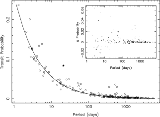
Figure 4.— The geometric transit probability for a circular orbit (solid curve) along with the transit probability for 203 RV planets from Butler et al. (2006) calculated from their orbital parameters (open circles). HD 17156b is indicated by a 5-pointed star. The sub-panel plots the difference in $P_{t}$ between the the actual orbit and a hypothetical circular orbit for each of the planets.

HD 17156b, a transiting planet with 21.2 day period (Barbieri et al., 2007), is shown as a 5-pointed star. Its transit probability is greatly increased by its orbital parameters. Note that the actual $P_{t}$ of HD 17156b is larger than the 5% shown in Figure 4 since the radius of the host star is 1.47 $R_{\sun}$. At longer periods, the planets with the largest residuals are HD 156846b, HD 4113b, and HD 20782b, which have periods of 359.51, 526.62, and 585.86 days, respectively. The probability residuals for these three planets are 0.024, 0.032, and 0.025 respectively, the effect of which is to raise their transit probabilities to the same level as HD 17156b if it were in a circular orbit. It is worth noting that these three planets all have eccentricities close to 0.9 which is undoubtedly the primary cause of the increased transit probability.

The increased transit probabilities of eccentric planets motivate photometric follow-up programs of RV planets. Compared to transit surveys, such programs require much less telescope time since the time of transit is, in principle, known. However, it was shown by Kane (2007) that reliable constraints on $e$ and $\omega$ are needed to avoid significant offsets in predicted transit times. This is particularly true of long period planets. In the case of planets HD 156846b, HD 4113b, and HD 20782b, the uncertainties cited in Butler et al. (2006) indicate that the values of $e$ are all constrained to $\pm 0.03$ and the values of $\omega$ are constrained to $\pm 3.0$°(compared to the mean and median values for all 203 planets of $\delta\omega=20\arcdeg$ and 10°, respectively). Thus, ephemerides for these planets can relatively reliably be determined from RV fit parameters alone. The transit duration is on the order of 12 hours for these planets, ensuring that one will practically never observe both the ingress and the egress of the transit during a single orbit from the ground. However, the large transit duration and relative low uncertainties in $e$ and $\omega$ will increase the chances of observing at least a partial transit during the predicted observing window.

3. Constraining Orbital Parameters

In §2, we discussed transit probability as a function of various system parameters as well as aspects of potential photometry follow-up campaigns. Here we focus on what can be learned from the presence and absence of a planetary transit in follow-up observations.

For a transiting planet the physical properties (such as the mass, radius, and density) can be calculated, leading to determination of (as opposed to constraints on) system parameters of the planet. Furthermore, the orbital inclination can be compared with the plane of stellar rotation (Winn et al., 2007) and used to test planetary models regarding co-planar orbits.

However, even the absence of a planetary transit signature in photometric data can lead to interesting constraints on the orbital parameters. Below, we elaborate on these constraints and apply the results to the aforementioned Butler et al. (2006) sample of RV planets.

3.1. Orbital Radius versus Stellar Radius

One implicit assumption in the derivation of the transit probability by Borucki & Summers (1984) is that the planet remains well outside the star in order to produce the solid angle of the planet’s shadow (see also Barnes, 2007). As a result, the calculation of $P_{t}$ in Equation 5 becomes invalid for extreme orbits with a small semi-major axis and a high value of eccentricity (see §2.1).

To quantify this assumption, we use Equation 4 to calculate the maximum eccentricity, $e_{\mathrm{max}}$, allowed as a function of the planet-star separation in units of $a/R$ where $R\equiv R_{p}+R_{\star}$. Applying the constraint $r>R$ when $f=0$ (i.e., the planet is outside the star at periapsis) to Equation 4 results in

$$R=\frac{a(1-e_{\mathrm{max}}^{2})}{1+e_{\mathrm{max}}}$$ (6)

and thus,

$$e_{\mathrm{max}}=1-\frac{R}{a}.$$ (7)

Equation 7 is plotted in Figure 5 for values of $a/R$ ranging from 1 to 30. Also shown are dot-dashed lines which indicate the $a/R$ values for OGLE-TR-56b (Konacki et al., 2003), XO-5b (Burke, 2008), and HD 17156b.

The restrictions upon the maximum eccentricity begin to become significant for $a/R<10$, which encompasses most of the known transiting exoplanets. This restriction is purely based upon orbital dynamics and there are undoubtedly additional limitations on the eccentricity due to tidal effects in this region.

Figure 5.— The maximum orbital eccentricity, $e_{\mathrm{max}}$, plotted as a function of the planet-star separation in units of $a/R$ (see Equation 7) in order for a planet to remain outside the surface of its parent star. This requirement is purely based on system geometry and does not take into account tidal effects or planet-planet interactions, but requires that $a>R$ when $f=0$. Dot-dashed lines indicate values for $a/R$ for various transiting planets.

3.2. Orbital Inclination and Argument of Periastron

One of the primary advantages of observing an exoplanet transiting the host star is that it eliminates the ambiguity in the planetary mass created by the unknown orbital inclination angle, $i$. The precise value of the inclination can be derived from the impact parameter of the transit across the stellar disk, defined by

$$b\equiv\frac{a\cos i}{R_{\star}}$$ (8)

and measurable from the shape of the lightcurve and the planet-star radius ratio (Seager & Mallén-Ornelas, 2003). Due to the constraint placed on $i$ by the presence of transits, the true planetary mass will be within a few percent of the value as determined from RV measurements alone.

The data available for transiting planets from the Extra-solar Planets Encyclopaedia and from Torres, Winn, & Holman (2008) show that the current distribution of inclination angles extends from 90°to almost 78°. The transiting planets whose orbits feature numerically lower values of $i$ (i.e., more “face-on”) are dominated by the very hot Jupiters, such as OGLE-TR-56b which has an inclination of $78.8\arcdeg\pm 0.5\arcdeg$ (Pont et al., 2007).

Figure 6.— The maximum orbital inclination for a non-transiting planet as a function of the argument of periastron, $\omega$, for eccentricities of 0.0 (solid line), 0.3 (dashed line), and 0.6 (dotted line), plotted for periods of both 4.0 days and 50.0 days.

If, however, a planet is determined not to transit, then limits may be placed upon the orbital inclination if the eccentricity and argument of periastron are known from RV measurements. This results from re-expressing Equation 2 as follows:

$$\cos i=\frac{R_{p}+R_{\star}}{a(1-e\cos E)}.$$ (9)

Figure 6 shows the maximum inclination for various values of period, $e$, and $\omega$. These are calculated by holding period and $e$ fixed whilst varying $\omega$ using Equations 3 and 9. We further assume a Jupiter radius and a solar radius for the values of $R_{p}$ and $R_{\star}$ respectively. For non-transiting planets on orbits with $e\neq 0$ whose periastron is aligned towards the observer (i.e., $\omega\sim\pi/2$), Figure 6 shows that the constraint on the inclination can be as high as $i\leq 75\arcdeg$, depending upon the orbital period. This is particularly useful for those planets whose mass estimate places them close to the brown dwarf regime. Note that Equation 9 reduces to Equation 7 when $i=90\arcdeg$ and $\omega=\pi/2$, consistent with the requirement that the planet remain outside the star.

3.3. Orbital Inclination and Eccentricity

As we show in §3.2, the fact that a planet is found to not transit limits the possible combinations of $e$, $\omega$, and $i$. We now consider what constraints may be placed upon the orbital inclination for a non-transiting RV planet as a function of eccentricity for the specific examples of when the periapsis is aligned towards ($\omega\sim\pi/2$) and away from ($\omega\sim 3\pi/2$) the observer.

Figure 7 illustrates the range of orbital inclinations that are excluded for two orbits (shown edge-on) of non-transiting planets. Both of these orbits have the same semi-major axes but different eccentricities and are aligned such that $\omega=3\pi/2$ (i.e., periapsis occurs behind the star as seen from the observer). In this case, the range of possible values of $i$ increases with decreasing orbital eccentricity ($\phi_{1}>\phi_{2}$). The opposite is true when $\omega=\pi/2$. In fact, the inclination in that case is only constrained by the requirement that the planet remain outside the star during periapsis (Equation 7).

Figure 7.— An edge-on view of two planetary orbits with the same values of semi-major axis, showing the range of excluded inclinations for an orbit with low eccentricity (dotted lines; $\phi_{1}$) and high eccentricity (dashed lines; $\phi_{2}$) for which the planet does not transit the parent star. For $\omega=3\pi/2$, the range of possible inclinations decreases with increasing eccentricity.

Figure 8 graphically demonstrates these constraints by plotting Equation 9, except now we fix the period and $\omega$ and vary $e$. A Jupiter radius and a solar radius are assumed for the values of $R_{p}$ and $R_{\star}$ respectively. The lines in these plots represent the maximum values for $i$ for a non-transiting planet as a function of $e$. These calculations are performed for four different periods and the two aforementioned orientations of $\omega$: $\omega=\pi/2$; left panel; case (a), and $\omega=3\pi/2$; right panel; case (b). It is worth noting that case (a) in Figure 8 represents the physical constraint described in Figure 5, since Equation 9 reduces to Equation 7 for $\omega=\pi/2$, as stated above.

Figure 8.— Maximum orbital inclination as a function of $e$ for non-transiting planets, plotted for four different periods (see Equation 9). The left panel, case (a), is for $\omega=\pi/2$ and is based on the requirement that the planet remain outside the star (§3.1). The right panel, case (b), shows the situation for $\omega=3\pi/2$, and is based on the geometrical arguments outlined in §3.3 and shown in Figure 7. The location of the maximum eccentricities of the known transiting planets TrES-3 and TrES-4, given their parameters in Table 1 and assuming $\omega=3\pi/2$, are indicated by 5-pointed stars.

In case (a), for example, a non-transiting planet in a 4-day orbit with $e=0.4$ has a range of possible inclination angles of $i\leq 80^{\arcdeg}$. For larger values of $e$ (at any period), the periastron distance of the planet will become so small that almost all values of $i$ are possible, the maximum value of $e$ at each period being defined by Equation 7. The dependence of $i$ upon $e$ is weaker for case (b) (note different scale for the left panel in Figure 8) since the periastron passage now happens behind the star (Figure 2) as seen from the observer, and thus, the range of possible $i$-values is not very constrained by $e$.

We now consider a planet discovered using the transit method with known $i$, $a$, $R_{p}$, and $R_{\star}$, but unknown values for $e$ and $\omega$. Is it possible to constrain $e$ in this scenario? Using Equation 9, the eccentricity can be expressed as follows

$$e=\frac{1}{cosE}\left(1-\frac{R_{p}+R_{\star}}{a\cos i}\right).$$ (10)

However, there exists a degeneracy between $e$ and $\omega=f(E)$ such that one cannot place constraints on one parameter without knowledge of the other. Additionally, as shown in §3.2, the constraint upon $i$ is only limited by the orbital boundary defined by Equation 7 when $\omega=\pi/2$.

Therefore, a meaningful constraint may only be placed upon $e$ for values of $\omega$ for which the orbital inclination is greater than the maximum predicted for a circular orbit (i.e., the region above the solid line shown in Figure 6). For case (b) ($\omega=3\pi/2$), Equation 10 reduces to

$$e=\frac{R_{p}+R_{\star}}{a\cos i}-1.$$ (11)

As an example, consider the two known transiting planets TrES-3 and TrES-4. The fit parameters shown in Table 1 for the values of $R_{\star}$, $R_{p}$, $i$, and $a$ are those reported by the discovery papers for TrES-3 (O’Donovan et al., 2007) and TrES-4 (Mandushev et al., 2007). Also shown in Table 1 are the maximum eccentricities for both case (a) and case (b). For case (a), the maximum eccentricity is $\sim 0.8$ for both planets. For case (b), the maximum eccentricity for these two planets is 0.4–0.5 and are plotted in the right panel of Figure 8. In each case, the maximum eccentricities are remarkably similar because the longer period of TrES-4 is compensated by the relatively large radii of the star and planet.

Table 1Fit parameters for TrES-3 and TrES-4 from O’Donovan et al. (2007) and Mandushev et al. (2007) respectively, along with the calculated maximum eccentricities.

Parameter	TrES-3	TrES-4
$R_{\star}$	$0.802\pm 0.046$	$1.738\pm 0.092$
$R_{p}$	$1.295\pm 0.081$	$1.674\pm 0.094$
$i$	$82.15\pm 0.21$	$82.81\pm 0.33$
$a$	$0.0226\pm 0.0013$	$0.0488\pm 0.0022$
$e(\omega=\pi/2)$	$0.808\pm 0.083$	$0.818\pm 0.073$
$e(\omega=3\pi/2)$	$0.404\pm 0.041$	$0.451\pm 0.040$

3.4. Global Statistics

The total number of transiting planets discovered thus far via radial velocity surveys does not necessarily reflect the true number of transiting planets in this sample. At the time of writing, most of the known radial velocity planets have not been adequately monitored photometrically in order to rule out transits. We can estimate the number of planets that should be transiting, and determine the significance of a hypothetical null result from a photometric follow-up campaign by applying the results of this paper to the Butler et al. (2006) RV planet sample.

The host star properties and planetary orbital parameters provided by Butler et al. (2006) form the foundation of a Monte-Carlo simulation of the transit probabilities calculated from Equation 5. The planetary radii $R_{p}$ are assumed to be one Jupiter radius as used in previous sections. However, the stellar radii $R_{\star}$ are estimated individually from the values of $B-V$ provided by Butler et al. (2006), assuming the host stars are dwarf stars (Cox, 2000). The orbital elements $a$, $e$ and $\omega$ are directly extracted from Butler et al. (2006). Using these values, we calculate $P_{t}$ for each of the 203 stars in the sample and randomly determine if the planet transits. This yields an integer number of projected transits from the sample. By performing these calculations $\sim 100000$ times, we produce a probability distribution for the number of transiting planets expected from this sample, shown in Figure 9.

Figure 9.— The probability distribution (solid line) for the 203 planets in the Butler et al. (2006) sample, predicting the number of transiting planets based on their estimated orbital parameters. Over-plotted is a gaussian distribution (dashed line) using the mean and standard deviation of the simulation results.

The simulated probability distribution has a mean value of $\sim 4.5$ transits peaking at $P_{t}\sim 0.2$ with a standard deviation of $\sim 2.0$. For comparison, we also generated a gaussian distribution profile using this mean and standard deviation. The a priori probability that none of the planets in this sample transit their host star is $\sim 1$%. In fact, three of the planets in this sample are known to transit, specifically HD 17156b, GJ 436b, and HD 147506b. Hence the current number of transiting planets from this sample is almost 1$\sigma$ below the expectation.

We further note that the sample of RV planets is biased toward numerically higher values of $i$ since detection efficiency will increase with higher $i$ for a given RV precision. As such, the expected number of transiting planets in the sample should be regarded as a lower limit. Though the discrepancy between known and expected transiting planets is not significant in this low-number regime, it is nevertheless quantifiable, and we conclude that further transit discoveries in this sample are possible or even likely. Any such additional detections would, in turn, lead to further understanding of the respective observational biases of the RV and transit methods. For example, the observational bias leads to an observed difference between the period distributions of planets discovered by the transit method and the radial velocity method, as discussed in detail by Gaudi, Seager, & Mallen-Ornelas (2005).

4. Conclusions

It is still uncertain at this stage how many of the known radial velocity planets transit their parent stars. What is clear is that the eccentricity distribution of the known exoplanets will increase the transit likelihood, making detections for long-period planets, such as HD 17156b, feasible. We have shown in this paper that there is enough potential amongst longer period planets for transit detections to motivate a photometric monitoring campaign at the predicted times of transit for these targets. Fleming et al. (2008) have shown that long-period transiting planets may yet be discovered through ground-based transit surveys, particularly if data sets from different surveys are combined.

As pointed out by Barnes (2007), eccentric planets that have a periastron oriented away from the observer are far more likely to exhibit a secondary than a primary eclipse. The detection of such a secondary eclipse is considerably more challenging than for a primary eclipse since it relies on a minimum level of planetary flux and is best pursued at infrared wavelengths. The discussion in §3.3 shows that even an assumption of $\omega=3\pi/2$ can place constraints on the orbital inclination. A prime candidate for such a study is HD 80606b (Naef et al., 2001) which has a period of 111.87 days and an eccentricity of 0.927. Scaling Figure 1 to this period and eccentricity yields a secondary transit probability of $\sim 15$%.

Many of the results presented in this paper can easily be applied to any system since the results generally scale linearly with the sum of the stellar and planetary radii. Through applying these results to current and future radial velocity planet discoveries, one can choose targets for an efficient observing campaign which may help to discover long-period transiting planets and hence add invaluable information to planetary structure and formation theories.

References

- Anderson et al. (2008) Anderson, D.R., et al., 2008, MNRAS, 387, L4
- Armitage (2007) Armitage, P.J., 2007, ApJ, 665, 1381
- Barbieri et al. (2007) Barbieri, M., et al., 2007, A&A, 476, L13
- Barnes (2007) Barnes, J.W., 2007, PASP, 119, 986
- Bouchy et al. (2005) Bouchy, F., et al., 2005, A&A, 444, L15
- Borucki & Summers (1984) Borucki, W.J., Summers, A.L., 1984, Icarus, 58, 121
- Burke (2008) Burke, C.J., 2008, ApJ, 679, 1566
- Burke (2008) Burke, C.J., et al., 2008, ApJ, submitted (arXiv:0805.2399)
- Butler et al. (2006) Butler, R.P., et al., 2006, ApJ, 646, 505
- Charbonneau et al. (2000) Charbonneau, D., Brown, T.M., Latham, D.W., Mayor, M., 2000, ApJ, 529, L45
- Cox (2000) Cox, A.N., 2000, Allen’s Astrophysical Quantities (4th ed.; New York: AIP)
- Fleming et al. (2008) Fleming, S.W., Kane, S.R., McCullough, P.R., Chromey, F.R., 2008, MNRAS, 386, 1503
- Ford & Rasio (2008) Ford, E.B., Rasio, F.A., 2008, ApJ, in press (astro-ph/0703163)
- Ford et al. (2008) Ford, E.B., Quinn, S.N., Veras, D., 2008, ApJ, 678, 1407
- Gaudi et al. (2005) Gaudi, B.S., Seager, S., Mallen-Ornelas, G., 2005, ApJ, 623, 472
- Gillon et al. (2007) Gillon, M., et al., 2007, A&A, 472, L13
- Henry et al. (2000) Henry, G.W., Marcy, G.W., Butler, R.P., Vogt, S.S., 2000, ApJ, 529, L41
- Johns-Krull et al. (2008) Johns-Krull, C.M., et al., 2008, ApJ, 677, 657
- Kane (2007) Kane, S.R., 2007, MNRAS, 380, 1488
- Kane et al. (2007) Kane, S.R., Schneider, D.P., Ge, J., 2007, MNRAS, 377, 1610
- Konacki et al. (2003) Konacki, M., Torres, G., Jha, S., Sasselov, D.D., 2003, Nature, 421, 507
- Li et al. (2008) Li, C.-H., et al., 2008, Nature, 452, 610
- López-Morales (2006) López-Morales, M., 2006, PASP, 118, 716
- López-Morales et al. (2006) López-Morales, M., Morrell, N.I., Butler, R.P., Seager, S., 2006, PASP, 118, 1506
- Mandushev et al. (2007) Mandushev, G., et al., 2007, ApJ, 667, L195
- Marcy et al. (1997) Marcy, G.W., Butler, R.P., Williams, E., Bildsten, L., Graham, J.R., Ghez, A.M., Jernigan, G., 1997, ApJ, 481, 926
- Naef et al. (2001) Naef, D., et al., 2001, A&A, 375, L27
- O’Donovan et al. (2007) O’Donovan, F.T., et al., 2007, ApJ, 663, L37
- Pál et al. (2008) Pál, A., et al., 2008, ApJ, in press (arXiv:0803.0746)
- Pepe et al. (2004) Pepe, F., et al., 2004, A&A, 423, 385
- Pont et al. (2007) Pont, F., et al., 2007, A&A, 465, 1069
- Sato et al. (2005) Sato, B., et al., 2005, ApJ, 633, 465
- Seager & Mallén-Ornelas (2003) Seager, S., Mallén-Ornelas, G., 2003, ApJ, 585, 1038
- Shankland et al. (2006) Shankland, P.D., et al., 2006, ApJ, 653, 700
- Torres et al. (2008) Torres, G., Winn, J.N., Holman, M.J., 2008, ApJ, 677, 1324
- Winn et al. (2007) Winn, J.N., et al., 2007, ApJ, 665, L167