Generating mixtures of spatial qubits

Abstract

In a recent letter [Phys. Rev. Lett. 94, 100501 (2005)], we presented a scheme for generating pure entangled states of spatial qudits ($D$-dimensional quantum systems) by using the momentum transverse correlation of the parametric down-converted photons. In this work we discuss a generalization of this process to enable the creation of mixed states. With the technique proposed we experimentally generated a mixture of two spatial qubits.

, , , , ,

1 Introduction

The experimental generation of pure entangled states and their entanglement properties have been extensively explored [1, 2, 3, 4, 5, 6, 7, 8]. However, the generation and the quantum properties of mixed states have received much less attention, even though this is a very important problem. For instance, the recent experimental works done on the generation of mixtures of two polarized qubits (2-dimensional quantum systems) [9, 10, 11] showed, surprisingly, that for the same state purity there is a class of states which are more entangled than the Werner states [12].

Besides being a valuable tool that can bring highlights to our understanding of quantum mechanics, the controlled generation of mixed states can be seen as a technique for state engineering. As was demonstrated in Ref [9], partially entangled states can be obtained by introducing a controlled decoherence into pure maximally entangled states. Another perspective is that, in some experimental situations, like in quantum key distribution with polarized entangled photons, the loss of coherence of the quantum state is an intrinsic phenomenon and a limiting constraint [13]. Therefore, it would be of paramount importance if the studies of mixing states could show a solution to minimize the decoherence in these experiments.

In a recent work [6, 7] we showed, theoretically and experimentally, that one can use the photon pairs created by spontaneous parametric down-conversion to generate pure entangled states of $D$-dimensional quantum systems. It was the first demonstration of high-dimensional entanglement based on the intrinsic transverse momentum entanglement of type-II down-converted photons. Because the quantum space of these photons is defined by the number of different available ways for their transmission through apertures placed in their paths, we call them spatial qudits. In this present work, we discuss how a modification of the setup employed to create pure qudit entangled states can be used to generate mixed states. By using the proposed technique we generated mixed states of spatial qubits. Up to our knowledge this is the first time that non-polarized mixed states of qubits are generated. Besides this, we believe that this is also the first time that a simple experimental technique that allows the generation of mixed states of qudits is discussed.

2 Theory

2.1 The state of the down-converted photons transmitted through multi-slits

Spontaneous parametric down-conversion is a nonlinear optical process where one photon from the pump (p) laser beam incident to a crystal can originate two other photons, signal (s) and idler (i)[14]. The generated photon pairs are also called twin photons for being generated simultaneously with a very small temporal uncertainty [15]. In references [6, 7] we showed that the state of the parametric down-converted photons, when transmitted through identical multi-slits, with $d$ being the distance between two consecutive slits, and $a$ the half width of the slits (See Fig 1), can be written as

$$|\,{\Psi}\,\rangle=\sum_{l=-l_{D}}^{l_{D}}\;\sum_{m=-l_{D}}^{l_{D}}W_{lm}\;e^{i\frac{kd^{2}}{8z_{A}}(m-l)^{2}}\;|\,{l}\,\rangle_{{}_{\!\scriptstyle s}}\otimes|\,{m}\,\rangle_{{}_{\!\scriptstyle i}},$$ (1)

where $k$ is the wave number of the pump beam used to generate the twin photons and $l_{D}=(D-1)/2$. $D$ is the number of slits in these apertures. The function $W_{lm}$ is the spatial distribution of the pump beam at the plane of the multi slits ($z=z_{A}$) and at the transverse position $x=(l+m)d/2$

$$W_{lm}=W\left[\frac{(l+m)d}{2};z_{A}\right].$$ (2)

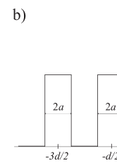
Figure 1: (a) Sketch of a 4-slits aperture. On the left side are shown the slit labels ($l$). (b) Transmission function of this aperture.

The $|\,{l}\,\rangle$ (or $|\,{m}\,\rangle$) state is a single-photon state defined, up to a global phase factor, by

$$|\,{l}\,\rangle_{{}_{\!\scriptstyle j}}\equiv\sqrt{\frac{a}{\pi}}\int\!\!d{q_{j}}\,e^{-iq_{j}ld}\mbox{\hskip 1.3ptsinc}\,(q_{j}a)|\,{1q_{j}}\,\rangle,$$ (3)

and represents the photon in mode $j$ ($j=i,s$)transmitted by the slit $l$. $|\,{1\mbox{\boldmath{${q}$}}_{j}}\,\rangle$ is the Fock state for one photon in mode $j$ with transverse wave vector $\mbox{\boldmath{${q}$}}_{j}$. The base $\{\,|\,{l}\,\rangle_{{}_{\!\scriptstyle j}}\}$ satisfies ${}_{{}_{\!\scriptstyle j}}\langle\,{l}\,|\,{l^{\prime}}\,\rangle_{{}_{\!\scriptstyle j}}=\delta_{ll^{\prime}}$. We use these states to define the logical states of the qudits and thus, it is clear that Eq. (1) represents a composite system of two qudits. Each qudit is represented by a vector in a Hilbert space of dimension $D$ because the degrees of freedom of each photon are the $D$ available paths for their transmission through the multi-slits.

It can be seen from Eq. (1) and Eq. (2) that it is possible to create different pure states of spatial qudits if one knows how to manipulate the pump beam in order to generate distinct transverse profiles at the plane of the multi-slits. In Ref. [7], for example , we showed experimentally that an entangled state of spatial ququads ($D=4$)

$$|\,{\Psi}\,\rangle=\frac{1}{2}\sum_{l=-\frac{3}{2}}^{\frac{3}{2}}e^{ik\frac{d^{2}l^{2}}{2z_{A}}}\;|\,{l}\,\rangle_{{}_{\!\scriptstyle s}}\otimes|\,{-l}\,\rangle_{{}_{\!\scriptstyle i}},$$ (4)

can be generated when the pump beam is focused at the plane of two identical four-slits in such a way that it is non-vanishing except in a region smaller than the dark part of these apertures.

2.2 Controlled generation of mixed states

Suppose now that, before reaching the crystal, the pump beam passes through an unbalanced Mach-Zehnder interferometer where the transverse profile of the laser beam is modified differently in each arm. If the difference between the lengths of these arms is set larger than the laser coherence length, we will obtain an incoherent superposition of the twin photon states generated by each arm. Whenever multi-slits are placed in the propagation paths of these photons, we will be generating a mixed state of two spatial qudits.

To generate a mixed state of two spatial qubits we performed the experiment outlined in Fig 2. A $5$ mm $\beta$-barium borate crystal is pumped by a $500$ mW krypton laser emitting at $\lambda=413$ nm for generating SPDC. Before being incident upon the crystal, the pump beam crosses an unbalanced Mach-Zehnder interferometer. The difference between the lengths of the interferometer arms ($200$ mm) is set larger than the laser coherence length ($80$ mm). Two identical double slits $A_{s}$ and $A_{i}$ are aligned in the direction of the signal and idler beams, respectively, at a distance of $200$ mm from the crystal ($z_{A}$). The slits’ width is $2a=0.09$ mm and their separation, $2d=0.18$ mm. At arm 1 of the interferometer we place a lens that focuses the laser beam at the plane of these double slits into a region smaller than $d$. In arm 2, we use a set of lenses that increases the transverse width of the laser beam at $z_{A}$. The transverse profiles generated are illustrated in Fig  2. The photons transmitted through the double-slits are detected in coincidence between the detectors $D_{i}$ and $D_{s}$. Two identical single slits of dimension $5.0$ x $0.1$ mm and two interference filters with $8$ nm full width at half maximum (FWHM) bandwidth are placed in front of the detectors.

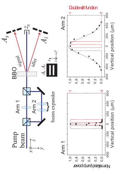
Figure 2: Schematic diagram of the experimental setup used for generating mixed states of spatial qubits. The pump beam that crosses arm 1 is focused at the plane of the double slits ($z=z_{A}$). When it passes through arm 2, it will be in a broader spatial region at this same plane. The transverse profiles generated are illustrated and compared with the double slit’s transmission function. $A_{s}$ and $A_{i}$ are the double-slits in signal and idler propagation paths, respectively.

Using Eq. (1) and Eq. (2), we can show that the two-photon state, after the double slits, when only arm 1 is open, is given by

$$|\,{\Psi}\,\rangle_{1}=\frac{1}{\sqrt{2}}(|\,{+}\,\rangle_{s}|\,{-}\,\rangle_{i}+|\,{-}\,\rangle_{s}|\,{+}\,\rangle_{i}).$$ (5)

To simplify, we used the state $|\,{+}\,\rangle_{j}$ ($|\,{-}\,\rangle_{j}$) to represent the $j$ photon being transmitted by the upper (lower) slit of the respective double slit (i.e., $l=+,-$). The state shown in Eq. (5) is a maximally entangled state of two spatial qubits.

However, if the laser beam crosses only arm 2, the state of the twin photons transmitted by the apertures will be

$$|\,{\Psi}\,\rangle_{2} = \frac{1}{2}\,e^{i\phi}(|\,{-}\,\rangle_{s}|\,{+}\,\rangle_{i}+|\,{+}\,\rangle_{s}|\,{-}\,\rangle_{i})$$ (6)

$$+\frac{1}{2}(|\,{-}\,\rangle_{s}|\,{-}\,\rangle_{i}+|\,{+}\,\rangle_{s}|\,{+}\,\rangle_{i}),$$

where $\phi=\frac{kd^{2}}{8z_{A}}$. The state $|\,{\Psi}\,\rangle_{2}$ is just partially entangled and, as was calculated in Ref [16], it has a concurrence [17] which is about three times weaker than the concurrence of the state $|\,{\Psi}\,\rangle_{1}$.

Therefore, the two-photon state generated in our experiment, when the two arms are liberated, is a mixed state of the spatial maximally entangled state of Eq. (5) and the state of Eq. (6). It is described by the density operator

$$\rho=A|\,{\Psi}\,\rangle_{{}_{\!\scriptstyle\,1\,1\!}}\langle\,{\Psi}\,|+B|\,{\Psi}\,\rangle_{{}_{\!\scriptstyle\,2\,2\!}}\langle\,{\Psi}\,|,$$ (7)

where $A$ and $B$ are the probabilities for generating the states of arm 1 and arm 2, respectively.

It is interesting to note that this generation can be completely controlled. Besides the fact that we can control the states generated in each arm (by controlling for each arm the pump beam transverse profile generated at the plane of the multi-slits), we also can control the probabilities $A$ and $B$ for generating the twin photon states. This is done by controlling the amount of pump power sent through each arm of the interferometer. For this purpose, we can replace the beam splitter at the entrance of the Mach-Zehnder interferometer by a polarizer beam splitter. Hence, a half wave plate in front of the pump beam before the interferometer allows us to propagate defined polarizations along the arms in such way that a rotation of the HWP behaves as a mechanism for a fine control of the fraction of the pump power sent through each arm. Furthermore, a HWP rotated at $45^{\circ}$ is inserted in the arm with horizontal polarization, so that photons arriving at the crystal have vertical polarization. This mechanism allows for pumping the non-linear crystal with a constant pump power.

3 Results and Discussion

The theory developed in the previous two sections, besides being quite appealing, is straightforward and now we show that our experimental results are in strong agreement with it. We stress that the subject of state determination [18, 19, 20, 21, 22, 23] of photonic states that are not defined in terms of the photon’s polarization is not trivial and, for this reason, the results here presented should be seen as a step forward in this study for spatial mixed states.

3.1 The probability of the basis states $\{|\,{l}\,\rangle_{{}_{\!\scriptstyle i}}|\,{l^{\prime}}\,\rangle_{{}_{\!\scriptstyle s}}\}$

The probability for the basis states $\{|\,{l}\,\rangle_{{}_{\!\scriptstyle i}}|\,{l^{\prime}}\,\rangle_{{}_{\!\scriptstyle s}}\}$ that appear in the coherent superposition of the states $|\,{\Psi}\,\rangle_{1}$ and $|\,{\Psi}\,\rangle_{2}$ can be measured directly. This is done with selective coincidence measurements recorded with the detectors placed just behind the double slit and it can be seen as a test of our theory, since one can infer from these probabilities the amplitudes of the coefficients of the states really generated by the the arms of the interferometer. In these measurements, the detector $D_{s}$ is kept fixed behind one slit while the other detector scans, in the $x$ direction, the entire region of its double slit. Two measurements of this kind with detector $D_{s}$ fixed behind the slit “+” ($l=+$) and then at the slit “-” ($l=-$), allow the determination of the probabilities for all the four basis states for the state of one of the interferometer’s arms . It should be clear that for measuring the amplitudes of the coefficients of $|\,{\Psi}\,\rangle_{1}$, the arm 2 should be blocked and vice-versa. To determine the coefficients of the other state, this procedure must be repeated.

According to the quantum state in Eq. (5), one is expected to have peaks of coincidences only when detector $D_{i}$ passes by the slit for which $l^{\prime}=-l$. However, for the state of arm 2 (Eq. (6)), coincidence peaks should happen with approximately the same number of coincidences between them, even when $l^{\prime}\neq-l$. The experimental data recorded is shown in Fig 3. One can clearly see that our results are in agreement with our theoretical predictions.

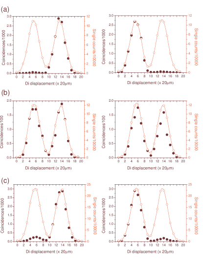
Figure 3: $D_{i}$ single counts ($\circ$) and coincidence counts ($\bullet$) measured in 20 s, simultaneously, with $D_{s}$ fixed behind one of the slits of its aperture. The data on the left side was recorded with $D_{s}$ fixed behind the slit “+” and on the right side with it fixed behind slit “-”. In (a) the measurements were done for determining part of the state of arm 1. This was done with arm 2 blocked. In (b) they were done for determining part of the state of arm 2. Arm 1 was blocked in this measurement. In (c) both arms are unblocked.

The general expression for the states that are more “likely” to have produced these results are, for arm 1

$$|\,{\Phi}\,\rangle_{1} = 0.077|\,{++}\,\rangle+0.704e^{i\phi}|\,{+-}\,\rangle$$ (8)

$$+0.699e^{i\phi}|\,{-+}\,\rangle+0.099|\,{--}\,\rangle,$$

whose fidelity with the state $|\,{\Psi}\,\rangle_{1}$ (Eq (5)) is $F=0.98\pm 0.05$. And for arm 2

$$|\,{\Phi}\,\rangle_{2} = 0.514|\,{++}\,\rangle+0.502e^{i\phi}|\,{+-}\,\rangle$$ (9)

$$+0.501e^{i\phi}|\,{-+}\,\rangle+0.483|\,{--}\,\rangle,$$

whose fidelity with the state $|\,{\Psi}\,\rangle_{2}$ is $F=1.00\pm 0.08$.

3.2 The Measurement of $A$ and $B$

The probabilities for generating the states $|\,{\Psi}\,\rangle_{1}$ ($A$) and $|\,{\Psi}\,\rangle_{2}$ ($B$) while both arms of the interferometer are unblocked can also be measured. And this measurement can also be used as a test for the theory given above.

We measured the values of $A$ and $B$ by blocking one of the arms of the interferometer and detecting the transmitted coincident photons through the signal and idler double-slits (See Fig 3). A (B) is the ratio between the total coincidence when arm 2 (arm 1) is blocked and the total coincidence when both arms are unblocked. From this measurement we obtained $A=0.85\pm 0.03$ and $B=0.15\pm 0.03$. The reason for having the probability of generating the state of arm 1 much higher than the probability for generating the state of arm 2 is quite simple. The laser beam that crosses arm 1 of the interferometer is focused at the slits’ plane and the spatial correlation of the generated photon pairs is such that it is more favorable to their transmission through the double slits than it is when the photon pairs are generated by the pump beam that crosses arm 2. These values of $A$ and $B$ can be properly manipulated by inserting attenuators at the interferometer.

This result can now be used for a test of our theory. To do this we must consider the detection of the fourth order interference patterns [14] at a transverse $z$-plane far behind the plane of the double slits. Since the state $|\,{\Psi}\,\rangle_{1}$ is a maximally entangled state, we would expect to observe strong conditional interference patterns [25, 26] for a mixture given by Eq (7) and with a high value of $A$, when both interferometer arms are unblocked. This would not be the case for high values of $B$, since the degree of entanglement of $|\,{\Psi}\,\rangle_{2}$ is at least three times smaller than the degree of $|\,{\Psi}\,\rangle_{1}$. The existence of a relation between the conditionality of the fourth-order interference patterns and the degree of entanglement of the two spatial qubit states was proven in Ref [16]. The interference patterns were recorded at a transversal plane that was $600$ mm behind the double slit’s plane. They were recorded as a function of the $D_{s}$ $x$-position and they are shown in Fig 4. In Fig 4(a), the idler detector was fixed at $x=0$ mm. In Fig 4(b), it was fixed at the transverse position $x=1376$ $\mu$m. The solid curves were obtained theoretically by using Eq (7) and the measured values of $A$ and $B$. The conditionality can be clearly observed in the interference patterns. One can also clearly see the good fit between the theoretical curve and our results.

Figure 4: Fourth order interference pattern as a function of $D_{s}$ position. In (a), the detector idler was fixed at the transverse position $x=0$ mm. In (b), it was fixed at the transverse position $x=1376$ $\mu$m. The solid curves were obtained theoretically.

As we discussed in the beginning of this section, these experimental observations corroborate the use of states $|\,{\Psi}\,\rangle_{1}$ and $|\,{\Psi}\,\rangle_{2}$ as good approximations for the states generated through arm 1 and arm 2 of the interferometer used.

4 Conclusion

In conclusion, we have shown that it is possible to generate a broader family of composite systems of spatial qudits by exploring the transverse correlations of the down-converted photons and the effects of optical interferometry. The process was discussed in detail and experimental evidences were shown that corroborate with the theory here proposed.

References

- [1] P. G. Kwiat, Klaus Matlle, H. Weinfurter, and A. Zeilinger, Phys. Rev. Lett. 75 (1995) 4337.
- [2] P. G. Kwiat et al. Phys. Rev. A 60 (1999) R773.
- [3] A. G. White et al. Phys. Rev. Lett. 83 (1999) 3103.
- [4] A. Vaziri, G. Weihs, and A. Zeilinger, Phys. Rev. Lett. 89 (2002) 240401.
- [5] J. Brendel, N. Gisin, W. Tittel, and H. Zbinden, Phys. Rev. Lett. 82 (1999) 2594.
- [6] L. Neves, S. Pádua and C. Saavedra Phys. Rev. A 69 (2004) 042305.
- [7] L. Neves, G. Lima, J. G. Aguirre Gómez, C. H. Monken, C. Saavedra, and S. Pádua, Phys. Rev. Lett. 94 (2005) 100501; Mod. Phys. Lett. B 20 (2006) 1.
- [8] J. C. Howell, A. Lamas-Linares, and D. Bouwmeester, Phys. Rev. Lett. 85 (2002) 030401.
- [9] A. G. White, D. F. V. James, W. J. Munro, and P. G. Kwiat, Phys. Rev. A 65 (2001) 012301.
- [10] N. A. Peters et al. Phys. Rev. Lett. 92 (2004) 133601.
- [11] M. Barbieri, F. De Martini, G. Di Nepi, and P. Mataloni, Phys. Rev. Lett. 92 (2004) 177901.
- [12] R. F. Werner, Phys. Rev. A 40 (1989) 4277.
- [13] A. Poppe et al., Opt. Express 12 (2004) 3865.
- [14] L. Mandel and E. Wolf, Optical Coherence and Quantum Optics, Cambridge University Press, Cambridge, 1995.
- [15] C. K. Hong, Z. Y. Ou, and L. Mandel, Phys. Rev. Lett. 37 (1987) 2044.
- [16] L. Neves, G. Lima, E. J. S. Fonseca, L. Davidovich, and S. Pádua, Phys. Rev. A 76 (2007) 032314.
- [17] W. K. Wootters, Phys. Rev. Lett. 80 (1998) 2245.
- [18] S. Wallentowitz and W. Vogel, Phys. Rev. Lett. 75 (1996) 2932.
- [19] T. J. Dunn, I. A. Walmsley and S. Mukamel, Phys. Rev. Lett. 74 (1995) 884.
- [20] K. Vogel and H. Risken, Phys. Rev. A 40 (1989) 2847.
- [21] D. T. Smithey et al., Phys. Rev. Lett. 70 (1993) 1244.
- [22] H. Kuhn, D. G. Welsch and W. Vogel, Phys. Rev. A 51 (1995) 4240.
- [23] D. F. V. James, P. G. Kwiat, W. J. Munro and A. G. White, Phys. Rev. A 64 (2001) 052312.
- [24] G. Lima, L. Neves, Ivan F. Santos, J. G. Aguirre Gómez, C. Saavedra and S. Pádua, Phys. Rev. A 73 (2006) 032340; Int. J. Q. Inf. 5 (2007) 69.
- [25] E. J. S. Fonseca, J. C. Machado da Silva, C. H. Monken, and S. Pádua, Phys. Rev. A 61 (2000) 023801.
- [26] D. M. Greenberger, M. A. Horne, and A. Zeilinger, Phys. Today 46 (1993) (8) 22.