High-order low-storage explicit Runge-Kutta schemes for equations with quadratic nonlinearities

Abstract

We show in this paper that third- and fourth-order low storage Runge-Kutta algorithms can be built specifically for quadratic nonlinear operators, at the expense of roughly doubling the time needed for evaluating the temporal derivatives. The resulting algorithms are especially well suited for computational fluid dynamics. Examples are given for the Hénon-Heiles Hamiltonian system and, in one and two space dimensions, for the Burgers equation using both a pseudo-spectral code and a spectral element code, respectively. The scheme is also shown to be practical in three space solving the incompressible Euler equation using a fully parallelized pseudo-spectral code.

.

1 Introduction

The explicit Runge–Kutta (ERK) method has a long and illustrious history in computational science and engineering. For example, these schemes are often selected in high spatial resolution studies of turbulence, in which the explicit nature of the scheme is used specifically in order to capture all time scales in the manner of direct numerical simulation (DNS). In the petascale era extremely high spatial resolutions can be reached, and improved accuracy in the time integration will also become necessary. The National Science Foundation has issued a baseline capability for its peta-scale initiative whereby a computation of homogeneous turbulence on a uniform grid of $12288^{3}$ points and at a Taylor Reynolds number $R_{\lambda}\sim 2000$ should be accomplished in forty wall clock hours. In view of the large arrays to be stored for such a computation, and in view of the large number of operations required in order to arrive at a time of order unity required for this initiative, it is clear that an accurate, low–storage and reasonably simple scheme is imperative if this challenge is to be met.

While there are many references to Runge-Kutta schemes in the scientific and engineering literature, we mention several that are of particular interest in this paper. It is well known that the standard fourth-order Runge-Kutta method can be evaluated using three levels of storage [1], and several low storage versions of Runge-Kutta methods are considered in [2]. In reference [3], new low storage methods adapted to acoustic problems is presented. Obviously, the stability of the integration schemes is an important issue. For high–order pseudo–spectral advection type problems this topic is also examined in detail in [4]; we consider here the problem of the stability of the algorithms empirically rather than from an analytical perspective.

In this work we begin with an algorithm (see Eq. 5 in Sec. (2.2)) which is attributed to Jameson, Schmidt and Turkel [5] in the text of [6]. We do not find this algorithm in [5], and are thus uncertain why the latter text would make this attribution. Nevertheless, we refer in the following to the algorithm given by Eq. (5) as the JST algorithm. Ostensibly, the JST algorithm requires only two levels of storage, but is of arbitrary order only for time–dependent linear problems. We show here that when the right hand side is nonlinear, corrections to the JST algorithm are needed if one wants to go beyond second order. The purpose of the present note is, after showing the limitations of the original algorithm, to compute the first corrections to the algorithm for quadratic nonlinearities as encountered for example in the modeling of incompressible flows. Our main result is that they can be implemented while preserving the low storage requirements.

The paper is organized as follows. Section 2 contains the general formulation of our new time-stepping algorithm. Numerical applications to conservative and dissipative systems are provided in Section 3. Finally, in Section 4 we present our conclusion.

2 General formulation

2.1 Basic definitions

Our starting point will be the following equation of motion for the vector ${\bf u}$

$${d{\bf u}\over{dt}}={\bf F}({\bf u}),$$ (1)

with

$${\bf F}({\bf u})={\bf L}({\bf u})+{\bf N}({\bf u},{\bf u}).$$ (2)

In what follows, all that we will explicitly require of ${\bf F}$ is the linearity of ${\bf L}$ and the fact that ${\bf N}$ is quadratic and symmetric in its arguments. The following considerations will thus be valid for any ${\bf L}$ satisfying

$${\bf L}(\lambda{\bf u_{1}}+\mu{\bf u_{2}})=\lambda{\bf L}({\bf u_{1}})+\mu{\bf L}({\bf u_{2}})$$ (3)

and quadratic ${\bf N}$ satisfying

$${\bf N}({\bf u_{1}},{\bf u_{2}})={\bf N}({\bf u_{2}},{\bf u_{1}}).$$ (4)

The main applications we have in mind are high order spatial discretizations of the Navier-Stokes equation, the incompressible Euler equation (Eq. 16), the magnetohydrodynamics (MHD) equations, or similarly nonlinear systems. Thus, the (real) vector ${\bf u}$ represents all of the (complex) components (modes) ${\hat{v}}_{\alpha}({\bf k})$ in a pseudo–spectral treatment, or all nodal or modal values in a spectral element or other high–order discretization. In these cases ${\bf L}$ and ${\bf N}$ can be obtained readily from the relevant terms in the discrete systems. Naturally, the same schemes may be useful in low order or fixed truncation methods as well.

2.2 JST loop

All of our new algorithms start by using the current value of the field ${\bf u}={\bf u}(t)$, to compute the order-$s$ JST loop [6]

$${\bf u}^{*}\leftarrow{\bf u}~{}$$

$$\ {\rm For\ }k=s,1,-1~{}$$

$$\ {\bf u}^{*}\leftarrow{\bf u}+\Delta t\frac{{\bf F}({\bf u}^{*})}{k}~{}$$

$$\ {\rm End\ For}~{}.$$ (5)

The original order-$s$ JST algorithm [6] simply amounts to setting, after the JST loop 5,

$${\bf u}^{\rm JST}(t+\Delta t)={\bf u}^{*}.$$ (6)

In the special case of linear ${\bf F}$, where ${\bf N}=0$, this algorithm can be obtained directly by factorizing the Taylor expansion

$${\bf u}(t+\Delta t)={\bf u}(t)+\sum_{k=1}^{s}(\Delta t)^{k}\frac{{\bf u^{(k)}}(t)}{k!}+\mathcal{O}(\Delta t^{s+1})$$ (7)

into

$${\bf u}(t+\Delta t)=\prod_{k=1}^{s}(1+\frac{\Delta t}{k}\frac{d}{dt}){\bf u}(t)$$ (8)

and is therefore exact. However, it is easy to check by explicit computation that when ${\bf N}\neq 0$, errors are present, beginning at order $3$ for $s\geq 3$.

Indeed, defining the error term by

$$\delta{\bf u}={\bf u}^{\rm JST}(t+\Delta t)-{\bf u}^{\rm exact}(t+\Delta t)\ ,$$ (9)

it is straightforward to obtain explicit Taylor expansions in time for both ${\bf u}^{\rm exact}(t+\Delta t)$ and ${\bf u}^{\rm JST}(t+\Delta t)$ respectively from the evolution equation (Eq. 1) and the definitions (Eq. 5) and (Eq. 6), and compute the difference (Eq. 9). For example, using obvious index notation for the rank-$n$ vectors ${\bf u}$ and ${\bf F}$, we obtain for the $i$ component when $s\geq 3$

$$\delta u_{i}=-\frac{\Delta t^{3}}{24}\sum_{j,k=1}^{n}\frac{\partial F_{i}}{\partial u_{j}\partial u_{k}}F_{j}F_{k}+\mathcal{O}(\Delta t^{4}).$$ (10)

Note that this expression suggests that the local error is $\mathcal{O}(\Delta t^{3})$; in almost all problems of interest, we integrate to a finite time, so the global error will then be $\mathcal{O}(\Delta t^{2})$. The basic idea of the new algorithms we propose below is to modify the JST loop in order to cancel the $\mathcal{O}(\Delta t^{3})$ term (and higher order terms) in (Eq. 10) that arises in the presence of nonlinear terms in the evolution equation.

2.3 Correction terms

In the following it will be convenient to vary the number of iterations of the JSP algorithm independently of the order of the desired algorithm. As a result, we will refer to calculations made with the original algorithm at arbitraty iteration count $s$ as a JST-$s$ scheme. Recall that for nonlinear problems, all these algorithms have second order global truncation errors.

Using (Eq. 10) we immediately arrive at a new $3^{\rm rd}$–order algorithm setting, after $s=3$ JST iterations,

$${\bf u} \leftarrow{\bf L}({\bf u})+{\bf N}({\bf u},{\bf u})~{}$$ (11)

$${\bf u} \leftarrow 2{\bf N}({\bf u},{\bf u})~{}$$

$${\bf u}^{*} \leftarrow{\bf u}^{*}+\frac{\Delta t^{3}}{24}{\bf u}~{}$$

$${\bf u} \leftarrow{\bf u}^{*}~{}.$$

Empirically we find that by increasing the number of JST iterations at a given truncation order, the overall error of the result is reduced. This can be shown to be the result of partial cancellations in higher order tems in (Eq. 10). For example, if we use $s=4$ JST iterations (a JST-4 algorithm), and then apply the recipe (Eq. 11), we reduce the errors still further, even though the scheme is still manifestly $3^{\rm rd}$ order. We denote these cases with a $+$, where the number of $+$ following the order indicate how many extra JST iterations were done. As a result, the $3^{\rm rd}$–order method with $s=4$ is refered to as $3+$ in the discussion below.

Following the same procedure, we can compute $4^{\rm th}$–order correction terms. Higher order terms in (Eq. 10) can be canceled by making use of reasonable extra computational resources. Thus, a new $4^{\rm th}$–order algorithm requires that after the JST-4 algorithm we set

$${\bf u} \leftarrow{\bf L}({\bf u})+{\bf N}({\bf u},{\bf u})~{}$$ (12)

$${\bf u} \leftarrow{\bf u}+\frac{\Delta t}{2}[{\bf L}({\bf u})+2{\bf N}({\bf u^{*}},{\bf u})]~{}$$

$${\bf u} \leftarrow 2{\bf N}({\bf u},{\bf u})~{}$$

$${\bf u}^{*} \leftarrow{\bf u}^{*}+\frac{\Delta t^{3}}{24}{\bf u}~{}$$

$${\bf u}^{*} \leftarrow{\bf u}^{*}+\frac{\Delta t^{4}}{72}[{\bf L}({\bf u})+2{\bf N}({\bf u^{*}},{\bf u})]~{}$$

$${\bf u} \leftarrow{\bf u}^{*}~{}.$$

Again, if (Eq. 5) is executed for $5$ iterations before applying (Eq. 12), we generally see a reduction in the overall error; hence, this approach is called the $4+$ scheme.

Table 1 contains a summary of some of the different possibilities. The rows correspond to the number $s$ of JST loop iterations and the columns to the order of the correction terms (Eq. 11) or (Eq. 12). The number of evaluations of nonlinear terms and the order of the resulting method are indicated. Extra $+$ symbols follow the previously defined convention and are also related to the amount of error present in the numerical examples (cf. Sec. (3)).

$s$	No correction		Third order		Fourth order
	Order	$n_{\rm NL}$	Order	$n_{\rm NL}$	Order	$n_{\rm NL}$
2	$2^{\rm nd}$	2	*	*	*	*
3	$2^{\rm nd}+$	3	$3^{\rm rd}$	5	*	*
4	$2^{\rm nd}++$	4	$3^{\rm rd}+$	6	$4^{\rm th}$	8

Table 1: Number of evaluations of nonlinear terms $n_{\rm NL}$ and order of the method obtained with $s$ JST iterations (Eq. 5) using, respectively, no correction, $3^{\rm rd}$ order (Eq. 11), and $4^{\rm th}$ order (Eq. 12) correction terms.

3 Numerical results

We now test these new algorithms on both conservative and dissipative systems. The conservative systems are the $2$–degree–of–freedom classical mechanics Hénon–Heiles system and the full $3$-D spatially-periodic incompressible Euler equation. Two dissipative systems are described by the Burgers equation. The first dissipative example uses a standard 1-$D$ Fourier pseudo-spectral method, while the second a 2-$D$ spectral element method.

3.1 Conservative systems

3.1.1 Hénon-Heiles

The Hénon–Heiles Hamiltonian was introduced in 1964 [7] as a mathematical model of the chaotic motion of stars in a galaxy. It is one of the simplest Hamiltonian systems to display soft chaos in classical mechanics. The Hénon-Heiles Hamiltonian reads

$$E=\frac{\dot{x}^{2}+\dot{y}^{2}}{2}+\frac{x^{2}+y^{2}+2x^{2}y-\frac{2}{3}y^{3}}{2}.$$ (13)

The associated nonlinear nonintegrable canonical equations of motion that, of course, exactly conserve the total energy $E$ are

$$\ddot{x} = -x-2xy~{},$$

$$\ddot{y} = -y-x^{2}+y^{2}\ .$$ (14)

These equations are of the general quadratic form (Eq. 2), so the Hénon-Heiles system (Eq. 14) is thus perhaps one of the simplest non-trivial dynamical system in which to test our new algorithms.

Figure 1 displays the numerical time-evolution of the relative error in the conserved energy $E(t)$ (Eq. 13), with $\Delta t=.001$ and initial data $x(0)=0$, $y(0)=0.12$, $\dot{x}(0)=0.486239$, $\dot{y}(0)=0.018$ corresponding to $E_{0}=.125$ for all cases. The error is computed as $(E(t)-E_{0})/E_{0}$.

It is apparent in the figure that the level of error decreases as the order of the method is increased. We note further that secular errors that are present in the third order method are canceled in the $3+$ case. As expected, the fourth order conservation is much more precise than the $3+$, in this case, at or below machine round–off.

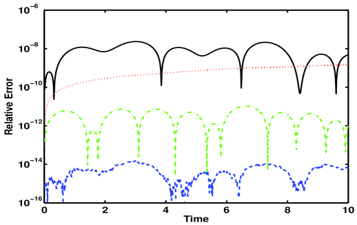
Figure 1: Relative error in energy versus time in the Hénon-Heiles system. Since the system is conservative, the error should be zero. Equations (Eq. 14) are solved and the resulting errors (Eq. 13) are shown corresponding to $2^{\rm nd}$–order ($3$ JST iterations; solid), $3^{\rm rd}$–order ($3$ JST iterations with correction; dotted), $3+$ ($4$ JST iterations with $3^{\rm rd}$–order correction; dash-dotted), and $4^{\rm th}$–order ($4$ JST iterations with $4^{\rm th}$–order corrections; dash).

3.1.2 Three-dimensional incompressible Euler equations

The (unit density) three-dimensional (3D) incompressible Euler equations,

$${\partial_{t}{\bf v}}+({\bf v}\cdot\nabla){\bf v} = -\nabla p~{},$$

$$\nabla\cdot{\bf v} = 0~{},$$ (15)

obeyed by a spatially $2\pi$-periodic velocity field can be approximated [6] by a (large) number of ordinary differential equations (ODEs) by performing a Galerkin truncation (${\bf\hat{v}}({\bf k})=0$ for $|{\bf k}|\leq k_{\rm max}$) on the Fourier transform ${\bf v}({\bf x},t)=\sum{\bf\hat{v}}({\bf k},t)e^{i{\bf k}\cdot{\bf x}}$.

One thus needs to solve the finite system of ODEs for the complex variables ${\bf\hat{v}}({\bf k})$ (${\bf k}$ is a 3D vector of relative integers $(k_{1},k_{2},k_{3})$ satisfying $|{\bf k}|\leq k_{\rm max}$)

$${\partial_{t}{\hat{v}}_{\alpha}({\bf k},t)}=-\frac{i}{2}{\mathcal{P}}_{\alpha\beta\gamma}({\bf k})\sum_{\bf p}{\hat{v}}_{\beta}({\bf p},t){\hat{v}}_{\gamma}({\bf k-p},t)\,,$$ (16)

where ${\mathcal{P}}_{\alpha\beta\gamma}=k_{\beta}P_{\alpha\gamma}+k_{\gamma}P_{\alpha\beta}$ with $P_{\alpha\beta}=\delta_{\alpha\beta}-k_{\alpha}k_{\beta}/k^{2}$ and the convolution in (Eq. 16) is truncated to $|{\bf k}|\leq k_{\rm max}$, $|{\bf p}|\leq k_{\rm max}$ and $|{\bf k}-{\bf p}|\leq k_{\rm max}$. This time-reversible system exactly conserves the kinetic energy $E=\sum_{k}E(k,t)$ and helicity $H=\sum_{k}H(k,t)$ where the energy and helicity spectra, $E(k,t)$ and $H(k,t)$, are defined by respectively averaging ${\frac{1}{2}}|{\bf\hat{u}}({\bf k^{\prime}},t)|^{2}\,$ and ${\bf\hat{u}}({\bf k^{\prime}},t)\cdot{\bf\hat{\omega}}({\bf-k^{\prime}},t)$ (with ${\bf\omega=\nabla\times{\bf u}}$ the vorticity) on spherical shells of width $\Delta k=1$.

Numerical solutions of equation (Eq. 16) are efficiently computed using a pseudo-spectral general-periodic code [8, 9] with $64^{3}$ Fourier modes that is dealiased using the standard $2/3$ rule [10] by spherical Galerkin truncation at $k_{\rm max}=21$. The code is fully parallelized with the message passing interface (MPI) library.

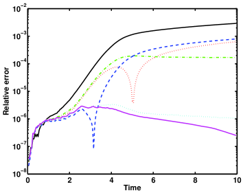
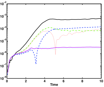
Figure 2: (left) Energy conservation in terms of relative error versus time. The incompressible Euler equation is solved using a dealiased pseudospectral method with resolution $64^{3}$. Results are shown for JST-$2$, -$3$, and -$4$ schemes (black, red dotted, and green dash-dotted curves, respectively), $3^{\rm rd}$–order (blue dashed), $3+$ (cyan dotted), and $4^{\rm th}$–order (solid magenta). (right) Helicity conservation in terms of relative error versus time, with curves representing the same schemes as for energy conservation.

The truncated Euler equation dynamics reaches, by way of progressive thermalization [11], an absolute equilibrium that is a statistically stationary gaussian exact solution of the associated Liouville equation [12]. Fig. 2 displays the energy and helicity conservation during this process. As in the previous section, the error in the conservation is measured as the relative difference in the energy (helicity) compared to that at $t=0$, as in Fig. 1.

The first thing we notice is that the original JST-$s$ scheme (5) has secular errors that are clearly visible for $s=2$ and $s=3$ but generally not as pronounced for $s=4$ at late time ($t>6$). We also observe that both JST–$3$ and the $3^{\rm rd}$–order schemes behave monotonically up to a certain time, then begin to increase its global error. In fact, the global error of the $3^{\rm rd}$–order algorithm begins to exceed that of the JST-$2$ and JST-$3$ schemes at around $t=4$. Before $t\approx 2.5$, however, we see convergence of the errors that behave with the new schemes roughly as they do in Fig. 1. As expected, we see the lowest errors when the method is increased to $4^{\rm th}$–order; however, it is clear that part of the errors present in the pure $3^{\rm rd}$–order scheme are canceled in the $3+$ case. Note that the $3+$ and $4^{\rm th}$–order schemes yield errors that decrease with time for this problem, a feature which may become important for very long integration times.

3.2 Dissipative systems

3.2.1 $1$D Burgers equation with a pseudospectral calculation

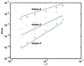
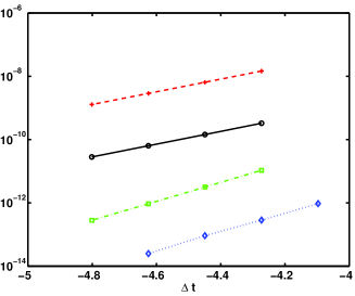
Figure 3: (left) Absolute error of the slope of the Burgers front $\sup_{x}(-\partial_{x}v)$ at $t=2$ versus time-step $\Delta t$. Burgers equation with initial data $\sin(x)$ is solved using a dealiased pseudospectral method with resolution $N=64$, $\nu=2\pi/N$. Results are shown for JST-$4$, (no corrections; circles), third order corrections (crosses), $3+$ (squares), and fourth order corrections (diamonds). Straight lines show the slopes indicating convergence orders 2, 3 and 4. (right) Absolute error in the area under the 1d curve (from [13]) vs time step for a spectral element N-wave solution to Burgers equation. Top red curve (slope $2.0017$): JST-$2$ algorithm; black curve: JST-$3$ (slope $2.0181$); green curve: $3^{\rm rd}$–order (slope $2.989$). The blue curve (bottom) uses the $3+$ algorithm (slope $2.9716$).

The $1$D Burgers equation

$$\partial_{t}u(x,t)+u(x,t)\partial_{x}u(x,t)=\nu\partial_{xx}u(x,t),$$ (17)

is of the general form (2). It is solved here using a standard pseudo-spectral code with $64$ Fourier modes, dealiased using the $2/3$ rule [10]. We run to $t=2$ by which time a sharp front has formed for the chosen initial conditions $u(x,t=0)=\sin x$, a front whose width is related to the viscosity, $\nu$. Each run is made with a different time step $\Delta t$, in order to check the truncation error as a function of $\Delta t$. We use as an error measure the absolute difference between the slope of the front in the numerical and analytical (see, e.g., [13]) solutions.

In Fig. 3 we present the Burgers front truncation errors. We see immediately that the errors decrease generally with an increase in the order of the scheme. In addition it is clear that here, as in Fig. 2, the $3+$ scheme, while still $3^{\rm rd}$–order, can produce global errors that are significantly lower than the $3^{\rm rd}$–order scheme alone.

3.2.2 $1$D Spectral elements

The spectral element method [14] combines the flexibility of finite elements with the spectral convergence of the pseudo–spectral method. Functions are expanded in each element in terms of Lagrange interpolating polynomials (here the Gauss–Lobatto–Legendre polynomials), and $\mathbb{C}^{0}$ continuity conditions are imposed on the element interfaces so that the functions reside in $\mathbb{H}^{1}$. The implementation we use is described in [15], and draws heavily from works by other investigators [16, 17, 18, 19, 20] in order to develop a new dynamic h–adaptive mesh refinement (AMR) formulation whereby the elements are subdivided isotropically according to a variety of a-posteriori refinement (and coarsening) conditions. The implementation sets the same polynomial degree in all elements, although this is not required of the method, and the polynomial degree can be varied for each run. The code forms a framework for solving a variety of PDEs. In addition, it is scalable, and is parallelized also by way of MPI. For this work, we use the nonlinear advection–diffusion solver, which solves the multi–dimensional Burgers equation. The solver allows the use of semi–implicit and explicit time stepping methods; an existing $2^{\rm nd}$–order JST method was modified to include trivially the third order correction terms (Eq. 11), with no additional storage.

For this test, we solve the N-wave problem [13] on a 2D mesh without adaptivity. The 2D Cole-Hopf transformation

$$u=-2\nu\vec{\nabla}\ln\chi$$ (18)

transforms (Eq. 17) into a heat equation for $\chi$. Choosing a source solution [13]

$$\chi(x,t)=1+\frac{a}{t}\exp-\frac{(x-x_{\,0})^{2}}{4\nu t},$$

we obtain the solution to (Eq. 17) immediately from (Eq. 18):

$$u(x,t)=\frac{x-x_{\,0}}{t}\frac{a}{a+t\exp((x-x_{\,0})^{2}/4\nu t)}.$$ (19)

This N-wave solution is essentially a 1D solution, but solved using a 2D solver with and without the new high order time integration schemes. We choose $\nu=0.1$, $a=0.01$, and initial time $t=0.04$, and integrate (Eq. 17) to $t=0.06$ using a polynomials of degree $8$ in each direction. In Fig. 3 we consider the absolute error in the area under the surface [13] vs time step in order to demonstrate the temporal convergence orders of the schemes.

4 Conclusion

We have shown that for quadratically nonlinear equations of motion the JST algorithm [5], [6] needs corrections to go beyond second order. We have computed the correction terms that enable the JST algorithm to be used for $3^{\rm rd}$- and $4^{\rm th}$-order truncation errors in non-linear quadratic equations, and we show that by utilizing the original JST algorithm, the new algorithm up to $4^{\rm th}$-order can be implemented with low storage requirements.

Numerical solutions to conservative and dissipative systems were used to verify the truncation errors of the new schemes, to verify their stability properties, and to demonstrate that they may be implemented easily using existing RK schemes. We considered implementations for a $3$D pseudo–spectral incompressible Euler code, a $1$D pseudo–spectral Burgers code, and a $2$D spectral element code. We find that the most cost effective method is the $3+$ scheme, which requires $4$ JST iterations and includes third order correction terms as described in the text.

A natural question to ask is whether such high order explicit integration schemes are required. We hinted at an answer in discussing our 3D results: for problems which are highly resolved spatially, as in pseudo–spectral or other spectrally convergent discretizations, the time error can come to dominate the dynamics. This is clearly the case in Fig. 2, which shows that a low order time integration scheme integrated for a long time could produce spurious conservation properties, yielding an unphysical result.

Acknowledgments

The National Center for Atmospheric Research is sponsored by the National Science Foundation.

References

- [1] E. K. Blum. A modification of the Runge-Kutta fourth-order method. Math. Comput., 16:176–187, 1962.
- [2] J. H. Williamson. Low storage Runge-Kutta schemes. J. Comput. Phys., 35:48–56, 1980.
- [3] M. Calvo, J. Franco, and L. Rández. A new minimum storage Runge–Kutta scheme for computational acoustics. J. Comput. Phys., 201(1):1–12, 2004.
- [4] J.L. Mead and R.A. Renaut. Optimal Runge-Kutta methods for first order pseudospectral operators. J. Comput. Phys., 152:404–419, 1999.
- [5] A. Jameson, W. Schmidt, and E. Turkel. Numerical solution of the Euler equations by finite volume methods using Runge-Kutta time stepping schemes. AIAA Paper, 81:1259, 1981.
- [6] C. Canuto, M. Y. Hussani, A. Quarteroni, and T. A. Zang. Spectral Methods in Fluid Dynamics. Springer-Verlag, New York and Berlin, 2nd printing edition, 1988.
- [7] M. Henon and C. Heiles. The applicability of third integral of motion: some numerical experiments. Astronomical Journal, 69(1):73–79, 1963.
- [8] D.O. Gómez, P.D. Mininni, and P. Dmitruk. Parallel simulations in turbulent MHD. Physica Scripta, 2005:123–127, 2005.
- [9] D.O. Gómez, P.D. Mininni, and P. Dmitruk. Mhd simulations and astrophysical applications. Advances in Space Research, 35:889–907, 2005.
- [10] D. Gottlieb and S. A. Orszag. Numerical Analysis of Spectral Methods. SIAM, Philadelphia, 1977.
- [11] C. Cichowlas, P. Bonaïti, F. Debbasch, and M.E. Brachet. Effective dissipation and turbulence in spectrally truncated Euler flows. Phys. Rev. Lett., 95(26), 2005.
- [12] S.A. Orszag. Analytical theories of turbulence. J. Fluid Mech., 41(363), 1970.
- [13] G. B. Whitham. Linear and Nonlinear Waves. Wiley, New York, 1974.
- [14] A. Patera. A spectral element method for fluid dynamics: laminar flow in a channel expansion. J. Comp. Phys., 54:468–488, 1984.
- [15] D. L. Rosenberg, A. Fournier, P. Fischer, and A. Pouquet. Geophysical-astrophysical spectral-element adaptive refinement (gaspar): Object-oriented h-adaptive fluid dynamics simulation. J. Comp. Phys., 215:59–80, 2006.
- [16] C. Mavriplis. Nonconforming discretizations and a posteriori error estimations for adaptive spectral element techniques. Ph.D. Disserataion, Massachusetts Institute of Technology, 1993.
- [17] R. D. Henderson. Dynamic refinement algorithms for spectral element methods. Comput. Methods Appl. Mech. Engrg., 175:395–411, 1999.
- [18] F. Loth P.F. Fischer, G. W. Kruse. Spectral element methods for transitional flows in complex geometries. J. Sci. Comp., 17:81–98, 2002.
- [19] H. Feng and C. Mavriplis. Adaptive spectral element simulations of thin flame sheet deformations. J. Sci. Comp., 17:1–3, 2002.
- [20] A. Patera. High-Order Methods for Incompressible Fluid Flow. Cambridge University Press, Cambrdige, 2002.