Measurements of time-dependent asymmetries in decays
B. Aubert
M. Bona
Y. Karyotakis
J. P. Lees
V. Poireau
E. Prencipe
X. Prudent
V. Tisserand
Laboratoire de Physique des Particules, IN2P3/CNRS et Université de Savoie, F-74941 Annecy-Le-Vieux, France
J. Garra Tico
E. Grauges
Universitat de Barcelona, Facultat de Fisica, Departament ECM, E-08028 Barcelona, Spain
L. LopezabA. PalanoabM. PappagalloabINFN Sezione di Baria; Dipartmento di Fisica, Università di Barib, I-70126 Bari, Italy
G. Eigen
B. Stugu
L. Sun
University of Bergen, Institute of Physics, N-5007 Bergen, Norway
G. S. Abrams
M. Battaglia
D. N. Brown
R. N. Cahn
R. G. Jacobsen
L. T. Kerth
Yu. G. Kolomensky
G. Lynch
I. L. Osipenkov
M. T. Ronan
K. Tackmann
T. Tanabe
Lawrence Berkeley National Laboratory and University of California, Berkeley, California 94720, USA
C. M. Hawkes
N. Soni
A. T. Watson
University of Birmingham, Birmingham, B15 2TT, United Kingdom
H. Koch
T. Schroeder
Ruhr Universität Bochum, Institut für Experimentalphysik 1, D-44780 Bochum, Germany
D. Walker
University of Bristol, Bristol BS8 1TL, United Kingdom
D. J. Asgeirsson
B. G. Fulsom
C. Hearty
T. S. Mattison
J. A. McKenna
University of British Columbia, Vancouver, British Columbia, Canada V6T 1Z1
M. Barrett
A. Khan
Brunel University, Uxbridge, Middlesex UB8 3PH, United Kingdom
V. E. Blinov
A. D. Bukin
A. R. Buzykaev
V. P. Druzhinin
V. B. Golubev
A. P. Onuchin
S. I. Serednyakov
Yu. I. Skovpen
E. P. Solodov
K. Yu. Todyshev
Budker Institute of Nuclear Physics, Novosibirsk 630090, Russia
M. Bondioli
S. Curry
I. Eschrich
D. Kirkby
A. J. Lankford
P. Lund
M. Mandelkern
E. C. Martin
D. P. Stoker
University of California at Irvine, Irvine, California 92697, USA
S. Abachi
C. Buchanan
University of California at Los Angeles, Los Angeles, California 90024, USA
J. W. Gary
F. Liu
O. Long
B. C. Shen
G. M. Vitug
Z. Yasin
L. Zhang
University of California at Riverside, Riverside, California 92521, USA
V. Sharma
University of California at San Diego, La Jolla, California 92093, USA
C. Campagnari
T. M. Hong
D. Kovalskyi
M. A. Mazur
J. D. Richman
University of California at Santa Barbara, Santa Barbara, California 93106, USA
T. W. Beck
A. M. Eisner
C. J. Flacco
C. A. Heusch
J. Kroseberg
W. S. Lockman
A. J. Martinez
T. Schalk
B. A. Schumm
A. Seiden
M. G. Wilson
L. O. Winstrom
University of California at Santa Cruz, Institute for Particle Physics, Santa Cruz, California 95064, USA
C. H. Cheng
D. A. Doll
B. Echenard
F. Fang
D. G. Hitlin
I. Narsky
T. Piatenko
F. C. Porter
California Institute of Technology, Pasadena, California 91125, USA
R. Andreassen
G. Mancinelli
B. T. Meadows
K. Mishra
M. D. Sokoloff
University of Cincinnati, Cincinnati, Ohio 45221, USA
P. C. Bloom
W. T. Ford
A. Gaz
J. F. Hirschauer
M. Nagel
U. Nauenberg
J. G. Smith
K. A. Ulmer
S. R. Wagner
University of Colorado, Boulder, Colorado 80309, USA
R. Ayad
Now at Temple University, Philadelphia, Pennsylvania 19122, USA
A. Soffer
Now at Tel Aviv University, Tel Aviv, 69978, Israel
W. H. Toki
R. J. Wilson
Colorado State University, Fort Collins, Colorado 80523, USA
D. D. Altenburg
E. Feltresi
A. Hauke
H. Jasper
M. Karbach
J. Merkel
A. Petzold
B. Spaan
K. Wacker
Technische Universität Dortmund, Fakultät Physik, D-44221 Dortmund, Germany
M. J. Kobel
W. F. Mader
R. Nogowski
K. R. Schubert
R. Schwierz
A. Volk
Technische Universität Dresden, Institut für Kern- und Teilchenphysik, D-01062 Dresden, Germany
D. Bernard
G. R. Bonneaud
E. Latour
M. Verderi
Laboratoire Leprince-Ringuet, CNRS/IN2P3, Ecole Polytechnique, F-91128 Palaiseau, France
P. J. Clark
S. Playfer
J. E. Watson
University of Edinburgh, Edinburgh EH9 3JZ, United Kingdom
M. AndreottiabD. BettoniaC. BozziaR. CalabreseabA. CecchiabG. CibinettoabP. FranchiniabE. LuppiabM. NegriniabA. PetrellaabL. PiemonteseaV. SantoroabINFN Sezione di Ferraraa; Dipartimento di Fisica, Università di Ferrarab, I-44100 Ferrara, Italy
R. Baldini-Ferroli
A. Calcaterra
R. de Sangro
G. Finocchiaro
S. Pacetti
P. Patteri
I. M. Peruzzi
Also with Università di Perugia, Dipartimento di Fisica, Perugia, Italy
M. Piccolo
M. Rama
A. Zallo
INFN Laboratori Nazionali di Frascati, I-00044 Frascati, Italy
A. BuzzoaR. ContriabM. Lo VetereabM. M. MacriaM. R. MongeabS. PassaggioaC. PatrignaniabE. RobuttiaA. SantroniabS. TosiabINFN Sezione di Genovaa; Dipartimento di Fisica, Università di Genovab, I-16146 Genova, Italy
K. S. Chaisanguanthum
M. Morii
Harvard University, Cambridge, Massachusetts 02138, USA
A. Adametz
J. Marks
S. Schenk
U. Uwer
Universität Heidelberg, Physikalisches Institut, Philosophenweg 12, D-69120 Heidelberg, Germany
V. Klose
H. M. Lacker
Humboldt-Universität zu Berlin, Institut für Physik, Newtonstr. 15, D-12489 Berlin, Germany
D. J. Bard
P. D. Dauncey
J. A. Nash
M. Tibbetts
Imperial College London, London, SW7 2AZ, United Kingdom
P. K. Behera
X. Chai
M. J. Charles
U. Mallik
University of Iowa, Iowa City, Iowa 52242, USA
J. Cochran
H. B. Crawley
L. Dong
W. T. Meyer
S. Prell
E. I. Rosenberg
A. E. Rubin
Iowa State University, Ames, Iowa 50011-3160, USA
Y. Y. Gao
A. V. Gritsan
Z. J. Guo
C. K. Lae
Johns Hopkins University, Baltimore, Maryland 21218, USA
N. Arnaud
J. Béquilleux
A. D’Orazio
M. Davier
J. Firmino da Costa
G. Grosdidier
A. Höcker
V. Lepeltier
F. Le Diberder
A. M. Lutz
S. Pruvot
P. Roudeau
M. H. Schune
J. Serrano
V. Sordini
Also with Università di Roma La Sapienza, I-00185 Roma, Italy
A. Stocchi
G. Wormser
Laboratoire de l’Accélérateur Linéaire, IN2P3/CNRS et Université Paris-Sud 11, Centre Scientifique d’Orsay, B. P. 34, F-91898 Orsay Cedex, France
D. J. Lange
D. M. Wright
Lawrence Livermore National Laboratory, Livermore, California 94550, USA
I. Bingham
J. P. Burke
C. A. Chavez
J. R. Fry
E. Gabathuler
R. Gamet
D. E. Hutchcroft
D. J. Payne
C. Touramanis
University of Liverpool, Liverpool L69 7ZE, United Kingdom
A. J. Bevan
C. K. Clarke
K. A. George
F. Di Lodovico
R. Sacco
M. Sigamani
Queen Mary, University of London, London, E1 4NS, United Kingdom
G. Cowan
H. U. Flaecher
D. A. Hopkins
S. Paramesvaran
F. Salvatore
A. C. Wren
University of London, Royal Holloway and Bedford New College, Egham, Surrey TW20 0EX, United Kingdom
D. N. Brown
C. L. Davis
University of Louisville, Louisville, Kentucky 40292, USA
A. G. Denig
M. Fritsch
W. Gradl
G. Schott
Johannes Gutenberg-Universität Mainz, Institut für Kernphysik, D-55099 Mainz, Germany
K. E. Alwyn
D. Bailey
R. J. Barlow
Y. M. Chia
C. L. Edgar
G. Jackson
G. D. Lafferty
T. J. West
J. I. Yi
University of Manchester, Manchester M13 9PL, United Kingdom
J. Anderson
C. Chen
A. Jawahery
D. A. Roberts
G. Simi
J. M. Tuggle
University of Maryland, College Park, Maryland 20742, USA
C. Dallapiccola
X. Li
E. Salvati
S. Saremi
University of Massachusetts, Amherst, Massachusetts 01003, USA
R. Cowan
D. Dujmic
P. H. Fisher
G. Sciolla
M. Spitznagel
F. Taylor
R. K. Yamamoto
M. Zhao
Massachusetts Institute of Technology, Laboratory for Nuclear Science, Cambridge, Massachusetts 02139, USA
P. M. Patel
S. H. Robertson
McGill University, Montréal, Québec, Canada H3A 2T8
A. LazzaroabV. LombardoaF. PalomboabINFN Sezione di Milanoa; Dipartimento di Fisica, Università di Milanob, I-20133 Milano, Italy
J. M. Bauer
L. Cremaldi
R. Godang
Now at University of South Alabama, Mobile, Alabama 36688, USA
R. Kroeger
D. A. Sanders
D. J. Summers
H. W. Zhao
University of Mississippi, University, Mississippi 38677, USA
M. Simard
P. Taras
F. B. Viaud
Université de Montréal, Physique des Particules, Montréal, Québec, Canada H3C 3J7
H. Nicholson
Mount Holyoke College, South Hadley, Massachusetts 01075, USA
G. De NardoabL. ListaaD. MonorchioabG. OnoratoabC. SciaccaabINFN Sezione di Napolia; Dipartimento di Scienze Fisiche, Università di Napoli Federico IIb, I-80126 Napoli, Italy
G. Raven
H. L. Snoek
NIKHEF, National Institute for Nuclear Physics and High Energy Physics, NL-1009 DB Amsterdam, The Netherlands
C. P. Jessop
K. J. Knoepfel
J. M. LoSecco
W. F. Wang
University of Notre Dame, Notre Dame, Indiana 46556, USA
G. Benelli
L. A. Corwin
K. Honscheid
H. Kagan
R. Kass
J. P. Morris
A. M. Rahimi
J. J. Regensburger
S. J. Sekula
Q. K. Wong
Ohio State University, Columbus, Ohio 43210, USA
N. L. Blount
J. Brau
R. Frey
O. Igonkina
J. A. Kolb
M. Lu
R. Rahmat
N. B. Sinev
D. Strom
J. Strube
E. Torrence
University of Oregon, Eugene, Oregon 97403, USA
G. CastelliabN. GagliardiabM. MargoniabM. MorandinaM. PosoccoaM. RotondoaF. SimonettoabR. StroiliabC. VociabINFN Sezione di Padovaa; Dipartimento di Fisica, Università di Padovab, I-35131 Padova, Italy
P. del Amo Sanchez
E. Ben-Haim
H. Briand
G. Calderini
J. Chauveau
P. David
L. Del Buono
O. Hamon
Ph. Leruste
J. Ocariz
A. Perez
J. Prendki
S. Sitt
Laboratoire de Physique Nucléaire et de Hautes Energies, IN2P3/CNRS, Université Pierre et Marie Curie-Paris6, Université Denis Diderot-Paris7, F-75252 Paris, France
L. Gladney
University of Pennsylvania, Philadelphia, Pennsylvania 19104, USA
M. BiasiniabR. CovarelliabE. ManoniabINFN Sezione di Perugiaa; Dipartimento di Fisica, Università di Perugiab, I-06100 Perugia, Italy
C. AngeliniabG. BatignaniabS. BettariniabM. CarpinelliabAlso with Università di Sassari, Sassari, Italy
A. CervelliabF. FortiabM. A. GiorgiabA. LusianiacG. MarchioriabM. MorgantiabN. NeriabE. PaoloniabG. RizzoabJ. J. WalshaINFN Sezione di Pisaa; Dipartimento di Fisica, Università di Pisab; Scuola Normale Superiore di Pisac, I-56127 Pisa, Italy
D. Lopes Pegna
C. Lu
J. Olsen
A. J. S. Smith
A. V. Telnov
Princeton University, Princeton, New Jersey 08544, USA
F. AnulliaE. BaracchiniabG. CavotoaD. del ReabE. Di MarcoabR. FacciniabF. FerrarottoaF. FerroniabM. GasperoabP. D. JacksonaL. Li GioiaM. A. MazzoniaS. MorgantiaG. PireddaaF. PolciabF. RengaabC. VoenaaINFN Sezione di Romaa; Dipartimento di Fisica, Università di Roma La Sapienzab, I-00185 Roma, Italy
M. Ebert
T. Hartmann
H. Schröder
R. Waldi
Universität Rostock, D-18051 Rostock, Germany
T. Adye
B. Franek
E. O. Olaiya
F. F. Wilson
Rutherford Appleton Laboratory, Chilton, Didcot, Oxon, OX11 0QX, United Kingdom
S. Emery
M. Escalier
L. Esteve
S. F. Ganzhur
G. Hamel de Monchenault
W. Kozanecki
G. Vasseur
Ch. Yèche
M. Zito
CEA, Irfu, SPP, Centre de Saclay, F-91191 Gif-sur-Yvette, France
X. R. Chen
H. Liu
W. Park
M. V. Purohit
R. M. White
J. R. Wilson
University of South Carolina, Columbia, South Carolina 29208, USA
M. T. Allen
D. Aston
R. Bartoldus
P. Bechtle
J. F. Benitez
R. Cenci
J. P. Coleman
M. R. Convery
J. C. Dingfelder
J. Dorfan
G. P. Dubois-Felsmann
W. Dunwoodie
R. C. Field
A. M. Gabareen
S. J. Gowdy
M. T. Graham
P. Grenier
C. Hast
W. R. Innes
J. Kaminski
M. H. Kelsey
H. Kim
P. Kim
M. L. Kocian
D. W. G. S. Leith
S. Li
B. Lindquist
S. Luitz
V. Luth
H. L. Lynch
D. B. MacFarlane
H. Marsiske
R. Messner
D. R. Muller
H. Neal
S. Nelson
C. P. O’Grady
I. Ofte
A. Perazzo
M. Perl
B. N. Ratcliff
A. Roodman
A. A. Salnikov
R. H. Schindler
J. Schwiening
A. Snyder
D. Su
M. K. Sullivan
K. Suzuki
S. K. Swain
J. M. Thompson
J. Va’vra
A. P. Wagner
M. Weaver
C. A. West
W. J. Wisniewski
M. Wittgen
D. H. Wright
H. W. Wulsin
A. K. Yarritu
K. Yi
C. C. Young
V. Ziegler
Stanford Linear Accelerator Center, Stanford, California 94309, USA
P. R. Burchat
A. J. Edwards
S. A. Majewski
T. S. Miyashita
B. A. Petersen
L. Wilden
Stanford University, Stanford, California 94305-4060, USA
S. Ahmed
M. S. Alam
J. A. Ernst
B. Pan
M. A. Saeed
S. B. Zain
State University of New York, Albany, New York 12222, USA
S. M. Spanier
B. J. Wogsland
University of Tennessee, Knoxville, Tennessee 37996, USA
R. Eckmann
J. L. Ritchie
A. M. Ruland
C. J. Schilling
R. F. Schwitters
University of Texas at Austin, Austin, Texas 78712, USA
B. W. Drummond
J. M. Izen
X. C. Lou
University of Texas at Dallas, Richardson, Texas 75083, USA
F. BianchiabD. GambaabM. PelliccioniabINFN Sezione di Torinoa; Dipartimento di Fisica Sperimentale, Università di Torinob, I-10125 Torino, Italy
M. BombenabL. BosisioabC. CartaroabG. Della RiccaabL. LanceriabL. VitaleabINFN Sezione di Triestea; Dipartimento di Fisica, Università di Triesteb, I-34127 Trieste, Italy
V. Azzolini
N. Lopez-March
F. Martinez-Vidal
D. A. Milanes
A. Oyanguren
IFIC, Universitat de Valencia-CSIC, E-46071 Valencia, Spain
J. Albert
Sw. Banerjee
B. Bhuyan
H. H. F. Choi
K. Hamano
R. Kowalewski
M. J. Lewczuk
I. M. Nugent
J. M. Roney
R. J. Sobie
University of Victoria, Victoria, British Columbia, Canada V8W 3P6
T. J. Gershon
P. F. Harrison
J. Ilic
T. E. Latham
G. B. Mohanty
Department of Physics, University of Warwick, Coventry CV4 7AL, United Kingdom
H. R. Band
X. Chen
S. Dasu
K. T. Flood
Y. Pan
M. Pierini
R. Prepost
C. O. Vuosalo
S. L. Wu
University of Wisconsin, Madison, Wisconsin 53706, USA
Abstract
We present new measurements of time-dependent asymmetries for
decays using pairs
collected with the BABAR detector located at the PEP-II Factory at
the Stanford Linear Accelerator Center. We determine the -odd
fraction of the decays to be and find asymmetry parameters and for the -even component
of this decay and and for the -odd component. We measure and for
, and for , and and for . For the decays, we also determine the -violating
asymmetry . In each case,
the first uncertainty is statistical and the second is systematic.
The measured values for the asymmetries are all consistent with the
Standard Model.
In the Standard Model (SM), violation is described by the
Cabibbo-Kobayashi-Maskawa (CKM) quark mixing matrix,
Cabibbo (1963); Kobayashi and Maskawa (1973). In particular, an
irreducible complex phase in the mixing matrix is the
source of all SM violation. Both the
BABAR Aubert et al. (2001) and Belle
Abe et al. (2001) collaborations have measured the parameter , where , in processes.
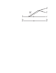
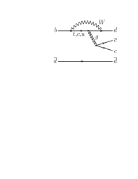
(a) Tree
(b) Penguin
Figure 1: Leading-order Feynman graphs for the decays.
The leading-order diagrams contributing to decays are
shown in Fig. 1, where the color-favored tree-diagram of
Fig 1(a) dominates. When neglecting the penguin (loop)
amplitude in Fig. 1(b), the mixing-induced asymmetry
of , denoted , is also determined by
Sanda:1996pm . The effect of neglecting the penguin
amplitude has been estimated in models based on factorization and
heavy quark symmetry, and the corrections are expected to be a few
percent Xing (1998, 2000). Large deviations of in
decays with respect to determined from
transitions could indicate physics beyond the
SM Grossman and Worah (1997); Gronau:2008ed ; Zwicky:2007vv .
The asymmetries of decays have been studied by both
the BABAR Aubert et al. (2007a, b) and
Belle Miyake et al. (2005); Aushev et al. (2004); Fratina et al. (2007)
collaborations. In the SM, the direct asymmetry , defined in
Sec. IV, for the decays is expected to be
near zero. The Belle Collaboration has observed a 3.2 sigma deviation
of from zero in the channel Fratina et al. (2007). This
has not been observed by BABAR nor has it been seen in other
decay modes, which involve the same quark-level
diagrams. As was pointed out in Gronau:2008ed , understanding
any possible asymmetries in these decays is important to constraining
theoretical models.
In this article, we update the previous measurements of asymmetry
parameters in decays Aubert et al. (2007a, b),
including the -odd fraction for , using the final
BABAR data sample. Charge conjugate decays are included implicitly
in expressions throughout this article unless otherwise indicated.
II Detector, data sample, and reconstruction
II.1 The BABAR detector
The data used in this analysis were collected with the BABAR detector Aubert et al. (2002a) operating at the PEP-II Factory located at
the Stanford Linear Accelerator Center (SLAC). The BABAR dataset
comprises pairs collected from 1999 to
2007 at the center-of-mass (CM) energy ,
corresponding to the resonance. We use
GEANT4-based Agostinelli et al. (2003) Monte Carlo (MC) simulation to
study backgrounds and to validate the analysis procedures.
The asymmetric energies of the PEP-II beams provide an ideal
environment to study time-dependent phenomena in the
system by boosting the in the laboratory frame, thus making
possible precise determination of the decay vertices of the two
meson daughters. BABAR employs a five-layer silicon vertex tracker
(SVT) close to the interaction region to provide precise vertex
measurements and to track low momentum charged particles. A drift
chamber (DCH) provides excellent momentum measurement of charged
particles. Particle identification of kaons and pions is primarily
derived from ionization losses in the SVT and DCH and from
measurements of photons produced in the fused silica bars of a
ring-imaging Cherenkov light detector (DIRC). A CsI(Tl) crystal-based
electromagnetic calorimeter enables reconstruction of photons and
identification of electrons. All of these systems operate within a
1.5 T superconducting solenoid, whose iron flux return is instrumented
to detect muons.
II.2 Candidate reconstruction and selection
The candidates used in this analysis are formed from oppositely
charged mesons where we include the decay modes
and and decay modes
, , ,
, and . In the mode, we reject candidates where both mesons decay to
because of its smaller branching fraction and larger
backgrounds. Reference Aubert et al. (2006) contains the details of
the reconstruction procedure, outlined here, used to select signal
candidates. Charged kaon candidates must be identified as such using
a likelihood technique based on the opening angle of the Cherenkov
light measured in the DIRC and the ionization energy loss measured in
the SVT and DCH Aubert et al. (2002a). We reconstruct candidates
from two oppositely charged tracks, geometrically constrained to a
common vertex and with an invariant mass within of the
nominal value Yao et al. (2006). We also require that the
probability of the vertex fit of the be greater than 0.1%. We
form candidates from a pair of photons detected in the
calorimeter, each with energy greater than . The invariant
mass of the two photons must be less than from the nominal
mass, and their summed energy must be greater than .
In addition, we apply a mass constraint to the candidates. We
require the reconstructed meson candidate mass to be within of the nominal value, except for the
decays where we use a looser requirement of . The
daughters of each candidate are fit to a common vertex with their
combined mass constrained to that of the meson. We use
candidates combined with a pion track with momentum less than in the CM frame to form candidates. We fit the decay with a vertex constraint.
Since the time of our previous
publications Aubert et al. (2007a, b, 2006), the
BABAR reconstruction routines have been extensively revised, leading
to significant improvements in localizing and reconstructing tracks,
particularly for low momentum charged particles. These improvements
have increased the reconstruction efficiency for final states with
multiple slow particles, such as the channel which has a
better than 20% improvement. As a result, the statistical
sensitivity of the measurements in this paper has increased more than
would be expected by just the increment in luminosity.
To suppress ()
continuum background, we exploit the spherical shape of events by
requiring the ratio of second to zeroth order Fox-Wolfram
moments Fox:1978vu to be less than . We select the candidates based on four variables: , where is the energy of the meson in the CM
frame, the candidate flight length significance, defined as the
sum of the two candidate flight lengths divided by the error on
the sum, a Fisher discriminant Asner et al. (1996), and a mass
likelihood of the mesons. The Fisher discriminant is a
linear combination of 11 variables: the momentum flow in nine
concentric cones around the thrust axis of the candidate, the
angle between the thrust axis and the beam axis, and the angle between
the line-of-flight of the candidate and the beam axis. The mass
likelihood is formed from Gaussian functions,
(1)
where the PDG subscript refers to the nominal
value Eidelman et al. (2004). The reconstructed masses and
uncertainties for the mesons prior to the
mass constraint are used in the likelihood. The portion of the
likelihood is the sum of two Gaussian functions, a central core and a
wider tail. The value of and the widths of the Gaussian functions are taken from detailed signal MC studies, which
show good agreement between data and MC samples. The selection
criteria are optimized for each decay channel to maximize the
total signal significance for each decay mode,
where and are the signal and background yields, respectively.
The optimized selections are specified in Aubert et al. (2006). We
keep candidates with ,
where is the momentum of the candidate in the CM frame.
On average 1.1–1.8 candidates per event satisfy all of the selection
criteria depending on the process. When more than one candidate
meets the selection criteria, the one with the best is kept.
We find from MC that this procedure retains the correct candidate more
than 95% of the time.
(a)
(b)
(c)
(d)
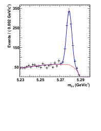
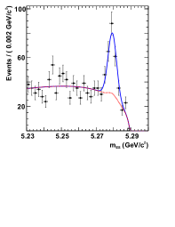
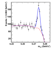
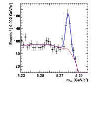
Figure 2: Projections of the fit results. The
solid line represents the total fit PDF and the dashed line is the
background contribution.
To determine the signal yields of the data sample, we use unbinned
maximum likelihood (ML) fits to the distributions. The signal is
described by a Gaussian function and the combinatorial background by a
threshold function Albrecht et al. (1990). In detailed MC studies of
the background, we find that there is a background contribution that
exceeds the threshold function in the region ,
where most of the signal events lie. We describe this component with
a Gaussian function having the same mean and width as the signal and
refer to it as peaking background because if neglected, it would lead
to an overestimate of the signal yields. In the channel,
the peaking background arises primarily from misreconstructed
events where the slow from the
decay is replaced by a to form a candidate. For the other three processes, our studies of the
composition of the peaking background show it to be consistent with
that of the combinatorial background in the region . We treat the peaking background component as an extension of
the combinatorial background. The peaking background yields relative
to the signal are fixed from MC to , ,
and for the , , and
modes, respectively, where the errors are due
primarily to the size of the MC sample available for background
studies. The signal mean and background shape are free parameters in
the fits. We fix the width of the signal Gaussian shape for and to 2.46 and 2.55 , respectively,
determined from MC, while the width of the signal is
allowed to float because of its much higher purity. The signal yields
are events, events, events, and events, where the
uncertainty is statistical only. The signal yields are consistent
with previously measured decay branching fractions from
BABAR Aubert et al. (2006) and
Belle Fratina et al. (2007); Abe:2002zy . When compared with past
BABAR measurements Aubert et al. (2006); Aubert:2005hs ; Aubert:2003ca ,
the low yield in Ref. Aubert et al. (2007a) is consistent
with a statistical fluctuation. The fit projections for each mode
onto are shown in Fig. 2.
III Time-integrated measurement of the -odd fraction
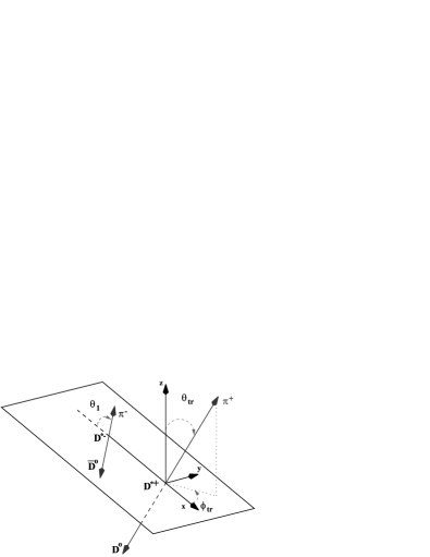
Figure 3: Depiction of the decay in the
transversity basis with the decay plane shown.
The three transversity angles are defined in the text.
The process has two vector mesons in the final state and
is an admixture of -even and -odd states depending on the
orbital angular momentum of the decay products. We measure the
-odd fraction using a time-integrated angular
analysis Dunietz et al. (1991). We define the three angles in the
transversity basis as depicted in Fig. 3: the angle
between the slow pion from the and the direction
opposite to the momentum in the rest frame; the polar
angle and the azimuthal angle of the slow
pion from the in the rest frame where the axis is
normal to the decay plane and the axis is opposite the
momentum. Working in the transversity basis, the
time-dependent angular distribution of the decay products is
(2)
where , with , represent time-dependent amplitudes
given by
(3)
Here, is the eigenvalue, for
, for ; is the parameter defined in Sec. IV; is the mixing
frequency, ; and is the lifetime, Yao et al. (2006). Expressions
similar to Eq. 2 hold for decays where
each is replaced by the appropriate including
. Integrating
Eq. 2 over , ,
and averaging over flavor while taking into account
detector efficiency yields
(4)
where we define
and . The three efficiency moments
are defined as
(5)
where ,
,
, and is the detector
efficiency. The moments are parameterized as second-order even
polynomials in whose parameters are determined from signal MC
simulation and fixed in the fit. The three functions deviate
only slightly from the same constant, making Eq. 4
nearly insensitive to , which we fix to zero in the fit.
Because is defined with respect to the slow pion from the
decay, the measurement resolution smears its distribution. We
convolve the function from Eq. 4 with a resolution
function which is modeled as the sum of
three Gaussian functions. In addition, we include an uncorrelated
Gaussian shape centered at and normalized in
to describe decays where the slow pion is poorly reconstructed leading
to a loss of angular information. The uncorrelated term represents
3% of the signal events where both slow pions are charged and around
16% in the modes where one of the slow pions is neutral. We
determine the parameters of the resolution model and of the
uncorrelated term from signal MC simulation and fix them in the ML
fit. Small differences observed in the angular distributions based on
the charge of the slow pions lead us to divide the efficiency moment
and resolution parameters into three categories, ,
, and .
We determine in a simultaneous unbinned ML fit to the and
distributions for the three slow-pion modes. The probability density function (PDF) was described in
Sec. II.2. The signal distribution is given
by Eq. 4 convolved with the resolution model. The
background distribution is modeled as a second-order even
polynomial , where ,
common to the three slow-pion modes, is allowed to float. The yield
for each of the three slow-pion modes is determined by the fit. We
validate the fitting procedure using high-statistics MC samples
divided into data-sized subsets and find no significant bias. Fitting
the data and including systematic uncertainties described below, we
find
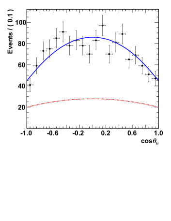
Figure 4: Projection of the fit result onto for events with . The solid line is the projected
fit result. The dashed line is the background component.
To evaluate the systematic uncertainty of , we vary the parameters
used to model the efficiency moments within the uncertainties of the
MC simulation used to extract them. We do the same for the parameters
used to model the experimental resolution. In both cases, we take
into account correlations among the parameters when perturbing the
values. We fix to zero in the nominal fit, so we also set it
to and assign the effect on the fitted result as a systematic
uncertainty. We change the and shapes of the peaking
background and assign the corresponding changes in as a systematic
uncertainty. We allow the background to have an additional
fourth-order term to test our assumption of this background shape.
This term is found to be consistent with zero, and we take the
difference in with respect to the nominal second-order background
description as the uncertainty with this model. We include as a
systematic uncertainty the statistical uncertainty associated with the
MC validation. A summary of the systematic uncertainties is found in
Table 1. The total systematic uncertainty is the sum
in quadrature of the individual contributions.
Table 1: Summary of systematic uncertainties on the
measurement of .
Angular efficiency moments
Angular measurement resolution
parameter uncertainty
Peaking background
background shape
Potential fit bias
Total
IV Time-dependent measurement
The decay rate () of the neutral meson to a common final
state accompanied by a () tag is
(7)
with asymmetry parameters , , and , where
() is the decay amplitude for () and
is the ratio of the flavor contributions to the mass
eigenstates Harrison and Quinn (1998). The parameter is the
average mistag probability, and is the difference
between the mistag probabilities for and . Here,
is the proper time
difference between the reconstructed as () and the used to tag the flavor ().
In the case of , we obtain an expression similar to
Eq. 7 from Eqs. 2
and 3,
The parameters in Eq. 3 need not be the same
because of possible differences in the relative contribution of
penguin and tree amplitudes, therefore the and parameters for
each of the three amplitudes can also differ. Note
that the minus sign before in the expression for absorbs
. We then define
In the absence of penguin contributions, , and . Because
is not a eigenstate, the expressions for
and are related, , where
is the strong phase difference between and decays Aleksan et al. (1993). Neglecting the penguin contributions,
, and .
The technique used to measure the time-dependent asymmetry is
discussed in detail in Ref. Aubert et al. (2002b). We calculate
between the two decays from the measured separation
of their decay vertices along the axis. The
decay vertex is determined from the daughter tracks of
the decay. The decay vertex is
determined in a fit of the charged tracks not belonging to
to a common vertex with a constraint on the beamspot
location and the momentum. Events that do not satisfy
and are
considered untagged in the time-dependent fit.
The flavor of the meson is determined using a
multivariate analysis of its decay products Aubert et al. (2002b). The
tagging algorithm classifies the flavor and assigns the candidate
to one of six mutually exclusive tagging categories based on the
output. A seventh untagged category is for events where the flavor
could not be determined. The performance of the tagging algorithm,
its efficiency and mistag rates, is evaluated using the time-dependent
evolution of a high-statistics data sample of , where the meson decays to
a flavor eigenstate and may be a , ,
or . The tagging algorithm has an efficiency
and an effective tagging
power .
The finite resolution of the vertex reconstruction smears the
distributions described in Eqs. 7
and 8. This measurement resolution is modeled as the sum
of three Gaussian functions described in Ref. Aubert et al. (2002b),
the parameters of which are also determined from the
sample.
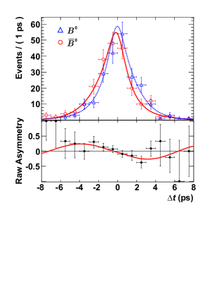
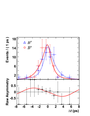
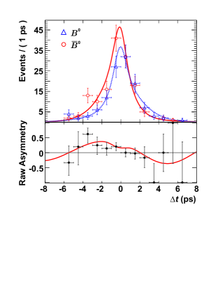
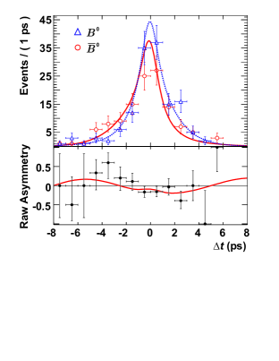
(a)
(b)
(c)
(d)
Figure 5: Projections onto of the fit
result and the data in the region for the
three highest purity tagging categories. The triangular points
and the dashed lines are for tagged events, and the circular
points and solid lines are for tagged events.
We determine the asymmetry parameters in unbinned ML fits to the
, , and in the case of , distributions.
The signal distributions are given in
Eqs. 7 and 8 convolved with the
experimental resolution. The background distribution has both
zero and nonzero lifetime components which are convolved with the
experimental resolution. The lifetime component is allowed to have
effective parameters and lifetime, which are determined in the
fits. The angular measurement resolution, determined for the -odd
fraction measurement, is convolved with the signal angular
distribution. The efficiency moments are not modeled but rather
absorbed into an effective , which is determined in the fit. This
procedure simplifies the distribution and does not introduce
a bias. The peaking background for the
channels shares the background distributions with the
combinatorial background because it originates from similar sources.
The peaking background has only a lifetime component,
since it originates from a specific decay. Untagged events are
also included in the fits to constrain the and shapes
but do not contribute to the determination of the parameters. We
also allow the signal yield, the background shape, and the
background shape to vary in the fits. Again we use
high-statistics MC samples divided into data-sized subsets to validate
the fitting procedure and find no significant bias.
The statistical uncertainties of the measurements below are
consistent with the expected uncertainties obtained from MC studies
that include the signal and background yields observed in data. The
statistical uncertainty for the channels is
essentially unchanged or even slightly worse than our previous
measurement Aubert et al. (2007a). We interpret this as a downward
fluctuation in the statistical uncertainty of the previous
measurement. Using MC data, we estimate the probability of observing
such a fluctuation at about 20%. For each measurement that follows,
the first uncertainty is statistical and the second is systematic.
From the fit to the data, we find
(11)
with an effective . If we perform the fit with
the additional constraints that
and , we obtain
(12)
having an effective . Fitting the data
yields
(13)
and fitting the data yields
(14)
Projections of the fit results onto for events in the region
, and their flavor asymmetry, can be seen in
Fig. 5. To enhance the visibility of the signal in
these projections, we use three of the six tagging categories with the
highest purity, which account for 80% of the total effective tagging
power . The correlations among the parameters are given in the
appendix.
Table 2: Systematic uncertainties on the parameters.
Tagging and resolution
0.022
0.031
0.010
0.017
0.021
0.009
Peaking background
0.012
0.079
0.002
0.019
0.012
0.003
Detector Alignment
0.006
0.029
0.001
0.019
0.005
0.002
Doubly-Cabibbo suppressed decays
0.002
0.002
0.014
0.014
0.002
0.014
Potential Fit Bias
0.011
0.098
0.008
0.065
0.011
0.007
Angular PDF variations
0.025
0.091
0.004
0.015
0.011
0.001
Other
0.013
0.025
0.005
0.029
0.013
0.002
Total
0.040
0.163
0.020
0.080
0.032
0.018
Table 3: Systematic uncertainties on the parameters.
Tagging and resolution
0.031
0.011
0.027
0.012
0.029
0.011
signal width
0.034
0.020
0.013
0.018
0.028
0.012
Peaking background
0.018
0.007
0.014
0.023
0.030
0.013
Detector Alignment
0.002
0.001
0.004
0.002
0.002
0.001
Doubly-Cabibbo suppressed decays
0.002
0.014
0.002
0.014
0.002
0.014
Potential Fit Bias
0.007
0.005
0.008
0.006
0.008
0.006
Other
0.006
0.002
0.002
0.006
0.004
0.003
Total
0.051
0.028
0.034
0.036
0.051
0.026
We evaluate systematic uncertainties in the asymmetries for each
mode by varying the fixed parameters for the mistag quantities and
resolution model within their uncertainties while accounting
for correlations among the parameters. For the and
modes, we change the fixed signal width by
, an amount determined from a comparison of data and MC
event samples in modes with high purity, and take the difference in
fitted results as a systematic uncertainty. Additionally, we vary the
fraction and shape of the peaking background component. We also
include systematics for possible detector misalignment and the
presence of doubly-Cabibbo suppressed decays of the
meson Long et al. (2003). We assign a systematic uncertainty equal to
the statistical uncertainty of the MC sample used to validate the fit.
Other sources of systematic uncertainty include: the meson
properties ( and ), which we vary to of their world averages, and uncertainty in the boost; the
corresponding changes in the asymmetries are taken as the estimate
of the systematic uncertainties. For the mode, we vary
the resolution parameters and background shape in the manner
described for the evaluation of systematic uncertainties on and
take the effects on the parameters as the associated systematic
uncertainty. A summary of the systematic uncertainties for the parameters is given in Tables 2 and 3.
As before, the total systematic uncertainty is the sum in quadrature
of the individual contributions.
Because decays are not eigenstates, it is
illustrative to express the asymmetry parameters and in a
slightly different parametrization Aubert:2003wr
(15)
The and parameters characterize
mixing-induced violation related to the angle and
flavor-dependent direct violation, respectively. is insensitive to violation but is related to the
strong phase difference . describes the
asymmetry between the rates and . Using the results from
Eq. 14 and taking into account correlations among the
variables, we find
(16)
From the signal yields and
determined in the time-dependent fit described above, we also measure
the time-integrated asymmetry in decays,
defined as
(17)
We find
(18)
where the systematic uncertainty is dominated by track reconstruction
efficiency differences for positive and negative tracks (0.013).
There is also a small contribution from the signal width, peaking
background, and MC statistics (0.002).
V Conclusion
We have measured the asymmetry parameters for decays, including the -odd fraction in the channel,
using the final BABAR data sample. All of the parameters are
consistent with the value of measured in
transitions Aubert:2007hm and with the expectation from the
Standard Model for small penguin contributions. The parameters
are consistent with zero in all modes. In particular, we see no
evidence of the large direct violation reported by the Belle
Collaboration in the channel Fratina et al. (2007). This
measurement supersedes the previous BABAR measurements Aubert et al. (2007a, b) of asymmetries in
these decays.
Acknowledgements.
We are grateful for the extraordinary contributions of our PEP-II colleagues in achieving the excellent luminosity and machine
conditions that have made this work possible. The success of this
project also relies critically on the expertise and dedication of the
computing organizations that support BABAR. The collaborating
institutions wish to thank SLAC for its support and the kind
hospitality extended to them. This work is supported by the U.S.
Department of Energy and National Science Foundation, the Natural
Sciences and Engineering Research Council (Canada), the Commissariat
à l’Energie Atomique and Institut National de Physique Nucléaire
et de Physique des Particules (France), the Bundesministerium für
Bildung und Forschung and Deutsche Forschungsgemeinschaft (Germany),
the Istituto Nazionale di Fisica Nucleare (Italy), the Foundation for
Fundamental Research on Matter (The Netherlands), the Research Council
of Norway, the Ministry of Education and Science of the Russian
Federation, Ministerio de Educación y Ciencia (Spain), and the
Science and Technology Facilities Council (United Kingdom).
Individuals have received support from the Marie-Curie IEF program
(European Union) and the A. P. Sloan Foundation.
*
Appendix A Correlations among the parameters
To allow detailed use of these results, we include the correlation
matrices for the parameters. Table 4 contains
correlations among the fit parameters in the channel with
separate -even and -odd asymmetries, and in the combined case,
the correlation between and
is with correlations to the effective the same as the
-even parameters. Table 5 contains the
correlations among the asymmetries. The
correlation of the time-integrated asymmetry with
any of the parameters is less than . The correlation
between and is .
Table 4: Correlations among the parameters
of the mode split by -even and -odd.
1
1
1
1
1
Table 5: Correlations among the parameters
of the mode.
1
1
1
1
References
Cabibbo (1963)
N. Cabibbo,
Phys. Rev. Lett. 10,
531 (1963).
Kobayashi and Maskawa (1973)
M. Kobayashi and
T. Maskawa,
Prog. Theor. Phys. 49,
652 (1973).
Aubert et al. (2001)
B. Aubert et al.
(BABAR Collaboration), Phys.
Rev. Lett. 87, 091801
(2001).
Abe et al. (2001)
K. Abe et al.
(Belle Collaboration), Phys. Rev.
Lett. 87, 091802
(2001).
(5)
A. I. Sanda and Z. Z. Xing,
Phys. Rev. D 56, 341 (1997).
Xing (1998)
Z. Z. Xing,
Phys. Lett. B443,
365 (1998).
Xing (2000)
Z. Z. Xing,
Phys. Rev. D61,
014010 (1999).
Grossman and Worah (1997)
Y. Grossman and
M. P. Worah,
Phys. Lett. B395,
241 (1997).
(9)
M. Gronau, J. L. Rosner and D. Pirjol,
Phys. Rev. D 78, 033011 (2008).
(10)
R. Zwicky,
Phys. Rev. D 77, 036004 (2008).
Aubert et al. (2007a)
B. Aubert et al.
(BABAR Collaboration), Phys.
Rev. Lett. 99, 071801
(2007a).
Aubert et al. (2007b)
B. Aubert et al.
(BABAR Collaboration), Phys.
Rev. D76, 111102
(2007b).
Miyake et al. (2005)
H. Miyake et al.
(Belle Collaboration), Phys.
Lett. B618, 34
(2005).
Aushev et al. (2004)
T. Aushev et al.
(Belle Collaboration), Phys. Rev.
Lett. 93, 201802
(2004).
Fratina et al. (2007)
S. Fratina et al.
(Belle Collaboration), Phys. Rev.
Lett. 98, 221802
(2007).
Aubert et al. (2002a)
B. Aubert et al.
(BABAR Collaboration), Nucl.
Instrum. Meth. A479, 1
(2002a).
Agostinelli et al. (2003)
S. Agostinelli
et al. (GEANT4 Collaboration),
Nucl. Instrum. Meth. A506,
250 (2003).
Aubert et al. (2006)
B. Aubert et al.
(BABAR Collaboration), Phys.
Rev. D73, 112004
(2006).
Yao et al. (2006)
W. M. Yao et al.
(Particle Data Group), J. Phys.
G33, 1 (2006).
(20)
G. C. Fox and S. Wolfram,
Phys. Rev. Lett. 41, 1581 (1978).
Asner et al. (1996)
D. M. Asner et al.
(CLEO Collaboration), Phys. Rev.
D53, 1039 (1996).
Eidelman et al. (2004)
S. Eidelman et al.
(Particle Data Group), Phys.
Lett. B592, 1
(2004).
Albrecht et al. (1990)
H. Albrecht et al.
(ARGUS Collaboration), Phys.
Lett. B241, 278
(1990).
(24)
K. Abe et al. (Belle Collaboration),
Phys. Rev. Lett. 89, 122001 (2002).
(25)
B. Aubert et al. (BABAR Collaboration),
Phys. Rev. Lett. 95, 131802 (2005).
(26)
B. Aubert et al. (BABAR Collaboration),
Phys. Rev. Lett. 90, 221801 (2003).
Dunietz et al. (1991)
I. Dunietz,
H. R. Quinn,
A. Snyder,
W. Toki, and
H. J. Lipkin,
Phys. Rev. D43,
2193 (1991).
Harrison and Quinn (1998)
P. F. Harrison and
H. R. Quinn
(BABAR Collaboration), The
BABAR physics book: Physics at an asymmetric factory
(1998), SLAC-R-0504, Papers from Workshop on
Physics at an Asymmetric B Factory (BABAR Collaboration Meeting), Rome,
Italy, 11-14 Nov 1996, Princeton, NJ, 17-20 Mar 1997, Orsay, France, 16-19
Jun 1997 and Pasadena, CA, 22-24 Sep 1997.
(29)
The order of the definition of these coefficients has changed since our previous publication Aubert et al. (2007b).
Aleksan et al. (1993)
R. Aleksan,
A. Le Yaouanc,
L. Oliver,
O. Pene, and
J. C. Raynal,
Phys. Lett. B317,
173 (1993).
Aubert et al. (2002b)
B. Aubert et al.
(BABAR Collaboration), Phys.
Rev. D66, 032003
(2002b).
Long et al. (2003)
O. Long,
M. Baak,
R. N. Cahn, and
D. Kirkby,
Phys. Rev. D68,
034010 (2003).
(33)
B. Aubert et al. (BABAR Collaboration),
Phys. Rev. Lett. 91, 201802 (2003).
(34)
B. Aubert et al. (BABAR Collaboration),
Phys. Rev. Lett. 99, 171803 (2007).