Warm Inflation and its Microphysical Basis
Abstract
The microscopic quantum field theory origins of warm inflation dynamics are reviewed. The warm inflation scenario is first described along with its results, predictions and comparison with the standard cold inflation scenario. The basics of thermal field theory required in the study of warm inflation are discussed. Quantum field theory real time calculations at finite temperature are then presented and the derivation of dissipation and stochastic fluctuations are shown from a general perspective. Specific results are given of dissipation coefficients for a variety of quantum field theory interaction structures relevant to warm inflation, in a form that can readily be used by model builders. Different particle physics models realising warm inflation are presented along with their observational predictions.
pacs:
98.80.Cq, 11.10.Wx, 12.60.Jvkeywords: cosmology, inflation, dissipation, particle production, supersymmetry
In Press Reports on Progress in Physics, 2009
I Introduction
It has been fourteen years since warm inflation was introduced and with it the first and still only alternative dynamical realisation of inflation to the standard scenario. The standard picture of inflation introduced in 1981 relied on a scalar field, called the inflaton, which during inflation was assumed to have no interaction with any other fields. During inflation, this field rolls down its potential and due to it being coupled to the background metric, a damping-like term is present which slows down its motion. As this inflaton field was assumed to not interact with other fields, there was no possibility for radiation to be produced during inflation, thus leading to a thermodynamically supercooled phase of the Universe during inflation. Getting out of this inflation phase and putting the Universe into a radiation dominated phase was a key issue, termed the “graceful exit” problem oldinf ; ni ; reheatu . The first successful solution of the graceful exit problem and so the first successful cold inflation model, was new inflation ni . The solution was to picture particle production as a distinct separate stage after inflationary expansion in a period called reheating. In this phase, couplings to other fields were assumed to be present and the inflaton would find itself in a very steep potential well in which it would oscillate. These oscillations would lead to a radiative production of particles. There have been many variants of the original cold inflation picture, first introduced in the context of the new inflation model and shortly afterwards in the chaotic inflation model ci , with many other models that followed.
The warm inflation picture differs from the cold inflation picture in that there is no separate reheating phase in the former, and rather radiation production occurs concurrently with inflationary expansion. The constraints by General Relativity for realising an inflationary phase simply require that the vacuum energy density dominates and so this does not rule out the possibility that there is still a substantial radiation energy density present during inflation. Thus on basic principles, the most general picture of inflation accommodates a radiation energy density component. The presence of radiation during inflation implies the inflationary phase could smoothly end into a radiation dominated phase without a distinctively separate reheating phase, by the simple process of the vacuum energy falling faster than the radiation energy, so that at some point a smooth crossover occurs. This is the warm inflation solution to the graceful exit problem.
Dynamically warm inflation is realised if the inflaton were interacting with other fields during the inflation phase. In fact in any realistic model of inflation, the inflaton must be coupled to other fields, since eventually the inflaton must release its vacuum energy to other fields thereby creating particles which form the subsequent radiation dominated era in the Universe. Thus the idea that these couplings to other fields somehow are inactive during inflation, as pictured in the cold inflation picture, is something that does require verifying by detailed calculation. When such calculations are done, the result is that there are regimes in which particle production during inflation occurs. This review will present the calculations which demonstrate particle production during inflation, thereby leading to a warm inflationary expansion.
The idea of particle production concurrent with inflationary expansion was first suggested in the pre-inflation inflation paper by L.Z. Fang in 1980 Fang:1980wi . His paper proposed using a scalar field with the origin of inflationary expansion due to a claimed anomalous dissipation term that would be generated based on Landau theory if the field was undergoing a second order phase transition. This was dynamically very different from the scalar field inflation that eventually became successful, and the source of dissipation was also different from that in warm inflation. However this model captured the basic idea of concurrent particle production and inflation. Then in the mid-80s two papers proposed adding a local type dissipation term into the evolution equation of the inflaton field, Moss im and then Yokoyama and Maeda Yokoyama:1987an . In both cases the dissipative term generated a source of radiation production during inflation. The idea of a dissipative term was re-discovered independently by Berera and Fang Berera:1995wh almost a decade later. They went further by proposing that the consistent dynamics of the inflaton field was a Langevin equation, in which a fluctuation-dissipation theorem would uniquely specify the fluctuations of the inflaton field. That paper by Berera and Fang provided the foundations for the theory of fluctuations in warm inflation and the Langevin equation has since been the fundamental equation governing inflaton dynamics. Following that work, in Berera:1995ie Berera proposed that a separate reheating phase, as standard in all inflation models up to then, could be eliminated altogether. This paper proposed a new picture of inflation, which it termed warm inflation, in which the process of inflationary expansion with concurrent radiation production could terminate simply by the radiation energy over-taking the vacuum energy, thus going from an inflationary to a radiation dominated era. This work presented an alternative solution to the graceful exit problem to the one given by the standard inflation scenario. This warm inflation picture was verified explicitly in Berera:1996fm , where the Friedmann equations for a Universe consisting of vacuum and radiation energy were studied and gave many exact warm inflation solutions to the graceful exit problem. Finally in Berera:1999ws the calculation of fluctuations were done by Berera for the inflaton evolving by a Langevin equation in a thermal inflationary Universe.
Alongside the development of the basic scenario, the first principles quantum field theory dynamics of warm inflation was developed. This started in Berera:1996nv with a quantum mechanical model which demonstrated the origin of the fluctuation-dissipation relation in warm inflation. The key step in deriving warm inflation from quantum field theory is in realising an overdamped regime for the evolution of the background inflaton field. The initial attempt at this was done by Berera, Gleiser and Ramos in BGR . In this work, it was proposed that the overdamped evolution should occur under adiabatic conditions in which the microscopic dynamical processes operated much faster than all macroscopic evolution, in particular the scalar field motion and Hubble expansion. Based on this criteria, a set of consistency conditions were formulated in BGR , which would be required for a self-consistent solution. However in BGR no explicit warm inflation solutions were found. This point was further highlighted by Yokoyama and Linde in Yokoyama:1998ju , in which several models were studied from which the conclusions of BGR were verified. The problem in these early works was that dissipation effects were being looked at in a high temperature regime and it proved too difficult to keep finite temperature effective potential corrections small, so that the inflaton potential remained relatively flat, and at the same time obtain a large dissipative coefficient. One type of model was shown that could realise such requirements BGR2 and this was the first quantum field theory model of warm inflation, although it was not a very compelling model. Subsequently Berera and Ramos in BR1 suggested a solution for getting around the mutual constraints of obtaining a large dissipative coefficient and yet small effective potential corrections. The main observation was that supersymmetry can cancel local quantum corrections, such as zero temperature corrections to the effective potential, whereas temporally non-local quantum effects, such as those that underly the dissipative effects, will not be cancelled. This led to BR1 proposing a two-stage interaction configuration, in which the inflaton was coupled to heavy “catalyst” fields with masses larger than the temperature of the Universe and these fields in turn were coupled to light fields. The evolution of the inflaton would induce light particle production via the heavy catalyst fields. Since these heavy catalyst fields were basically in their ground state, the quantum corrections associated with them could be cancelled in supersymmetric models. The calculation of the low temperature dissipative coefficients for this two-stage mechanism were first done by Moss and Xiong mx .
There is an earlier review which covered the basics of the warm inflation scenario Berera:2006xq . In this review full details will be developed of the quantum field theory dynamics of warm inflation. This will first start in Sec. II with a summary of the warm inflation scenario, including a comparison of it to cold inflation. In Sec. III a basic introduction to thermal field theory is given including the real time formalism for interacting field theories. In Sec. IV the effective evolution equation of the inflaton field is derived, in which all fields it interacts with are integrated out, leading to a Langevin type nonconservative equation which contains a dissipative term and a noise force term. The detailed properties of these dissipation and fluctuation terms is then studied in Sec. V. In addition the physical picture of the dissipation effects in warm inflation are discussed. In Sec. VI the calculations are extended to curved spacetime. In Sec. VII various particle physics models of warm inflation are presented. Finally Sec. VIII presents some concluding remarks and future work being done on the subject. Our conventions are as follows. We use spacetime metrics with signature, and we use natural units for the Planck’s constant, Boltzmann’s constant and the velocity of light .
II The Warm Inflation Picture and its Motivations
II.1 Background equations
The foundation of cosmology is the cosmological principle which states no observer occupies a preferred position in the Universe. This principle implies the Universe must be homogeneous (looks the same from every point) and isotropic (looks the same in all directions). To quantify the cosmological principle, in regards the geometry, the metric of a space-time which is spatially homogeneous and isotropic is given by the Friedmann-Robertson-Walker (FRW) metric,
| (1) |
where are spherical-polar coordinates parameterizing the spatial dimensions, is cosmic time, and describe spaces of constant positive, negative and zero spatial curvature. The most important quantity here is which is the cosmic scale factor and describes the expansion of the Universe. The Hubble parameter, defined by
| (2) |
quantifies how fast the Universe expands.
The evolution of the scale factor is related to the pressure and density by the scale factor acceleration equation,
| (3) |
where is Newton’s gravitational constant. Energy conservation is expressed by
| (4) |
Inflation by definition is a phase when the scale factor is growing at an accelerated rate, , which based on Eq. (3) requires , thus for a substance with negative pressure. The spatial part of the metric evolves rapidly towards the flat metric , and
| (5) |
The most common example of inflationary expansion occurs when the dominant form of matter has equation of state , which is called vacuum energy. Such an equation of state plugged into Eq (5) leads to an exponential scale factor behavior , with constant.
II.2 Inflaton dynamics
The key problem of inflationary cosmology has been trying to realise inflation from a realistic particle physics motivated model. The general observation which has driven this idea is that a scalar field has the necessary equation of state needed for inflation. In particular the energy and pressure density of a scalar field are, respectively, given by
| (6) |
with the key point being that the potential energy of this field has precisely the equation of state conducive to inflation. Thus, the basic idea has always been to somehow get the potential energy of a scalar field to dominate the energy density in the Universe, and thereby drive inflation. And then, once enough inflation has occurred, to convert the potential energy into radiation and enter into a radiation dominated expansion phase. There are two underlying dynamical realisations of inflation, into which all models fall, cold and warm inflation. Both dynamical pictures are summarized in Fig. 1 and this subsection will review both pictures.
II.2.1 Cold inflation
This is the standard picture of inflationary dynamics. In the cold inflationary picture, one or more scalar inflaton fields are assumed to decouple from everything apart from gravity. The energy density is dominated by the scalar field potential. For example, in Fig. 2 it is shown a potential, in which when the inflaton amplitude is displaced to some , inflation can occur. The evolution of the scalar field in the FRW universe is described by the General Relativistic version of the Klein-Gordon equation,
| (7) |
In this equation the Hubble damping term, , formally acts like a friction term that damps the inflaton evolution. However this term does not lead to dissipative energy production, since its origin is from the coupling of the scalar field with the background FRW metric. The inflaton plays the role of driving inflation as well as providing the seeds for density fluctuations. This Subsection only focuses on the first of these requirements.
In order for inflation to occur, the inflaton must be potential energy dominated, which means the potential energy must be larger than the gradient energy and the kinetic energy ,
| (8) |
Moreover, in order to obtain enough inflation, these conditions must persist for some span of time. The usual way to achieve this is for the inflaton to start out almost homogeneous and at rest in some small patch of space and then to have the inflaton evolution equation overdamped, with approximate form
| (9) | |||
| (10) |
The consistency of this approximation is governed by conditions on a set of two slow-roll parameters,
| (11) |
where , so GeV. If these conditions hold in a region of space, then inflation can happen.
For the inflaton dynamics described by Eq. (7), it is instructive to see how an inflationary scale factor growth occurs. It follows from the approximate Eqs. (9) and (10) that and therefore, for the expansion is roughly constant. From Eq. (10) we see that , where , as we stated earlier.
The evolution of any radiation contribution to the energy density in the universe also can be easily studied in this example. The energy conservation equation becomes , which has the exponentially decaying solution . In other words, whatever the initial radiation energy density in the universe at the onset of cold inflation, this rapidly decays away, thus supercooling the universe. As shown in Fig. 1, during cold inflation, the vacuum energy density is large and almost constant, whereas the radiation energy density is negligible, hence the name cold inflation.
Once a region of adequately large potential energy materializes, the physics of the subsequent evolution is quite straightforward. The gravitational repulsion caused by the negative pressure drives that region into a period of accelerated expansion. One expresses the amount of inflation as the ratio of the scale factor at the end of inflation to that at the beginning , and it is usually stated in terms of the number of e-folds ,
| (12) |
In order to inflate the horizon size to a scale covering the observable universe, it is necessary to have around 60 e-folds of inflation.
Eventually, inflation must end and radiation must be introduced into a very cold universe so as to put it back into a radiation dominated Hot Big Bang regime, which is the so called graceful exit problem oldinf ; ni ; reheatu . In the cold inflation picture, the process that performs this task is called reheating reheatu . This is usually envisioned as occurring shortly after the slow-roll approximation has broken down, and is often associated with oscillations of the inflaton field about the minimum of its potential. An example of this type of potential will be studied in more detail in Subsec. II.4. If the inflaton is interacting with other matter fields, the oscillations of the inflaton will lead to particle production so that, as shown in Fig. 1, the radiation energy density begins to increase.
II.2.2 Warm inflation
The other dynamical realisation of inflation is warm inflation. This picture is similar to cold inflation to the extent that the scalar inflaton field must be potential energy dominated to realise inflation. The difference is, in this picture the inflaton is not assumed to be an isolated, non-interacting field during the inflation period. So, rather than the Universe supercooling during inflation, instead the Universe maintains a small amount of radiation during inflation, enough to noticeably alter inflaton dynamics. In particular, the dividing point between warm and cold inflation is roughly at , where is the radiation energy density present during inflation and is the Hubble parameter. Thus is the warm inflation regime and is the cold inflation regime. This criterion is independent of thermalisation, but if such were to occur, one sees this criteria basically amounts to the warm inflation regime corresponding to when . This condition is easy to understand since the typical inflaton mass during inflation is and so when , thermal fluctuations of the inflaton field will become important. Subsequent to the introduction of warm inflation, other scenarios have been suggested which utilize some of its concepts such as thermal fluctuations during inflation Alexander:2001dr ; Magueijo:2002pg ; Ferreira:2007cb and graceful exit via radiation energy density that smoothly becomes dominant Alexander:2001dr ; however the dynamics in these scenarios differs from that of scalar field stochastic evolution.
The interaction of the inflaton with other fields implies its effective evolution equation in general will have terms representing dissipation of energy out of the inflaton system and into other particles. Berera and Fang Berera:1995wh initially suggested that for a consistent description of an inflaton field that dissipates energy, the inflaton evolution equation should be of the Langevin form, in which there is a fluctuation-dissipation relation which uniquely relates the field fluctuations and energy dissipation. This has formed the basis of all fluctuation calculations in warm inflation. The simplest such equation would be one in which the dissipation is temporally local,
| (13) |
In this equation, is a dissipative term and is a fluctuating force. Both are effective terms arising due to the interaction of the inflaton with other fields. In general these two terms will be related through a fluctuation-dissipation theorem, which would depend on the statistical state of the system and the microscopic dynamics. Equations like (13) are the main subject of this review, and will be further described in the next subsection and in Secs. III-V.
In order for warm inflation to occur the potential energy must be larger than both the radiation energy density and the inflaton’s kinetic energy. A major difference from cold inflation is in the evolution of the energy densities, as can be compared in Fig. 1. In warm inflation the radiation energy does not vanish because vacuum energy is continuously being dissipated at the rate . The energy conservation equation (4) for this system of vacuum and radiation becomes
| (14) |
In this equation the second term on the right-hand-side acts like a source term which is feeding in radiation energy, whereas the first term is a sink term that is depleting it away. When , and are slowly varying, which is a good approximation during inflation, there will be some nonzero steady state point for . Thus at large times, compared to the local Hubble time, the radiation in the universe becomes independent of initial conditions and depends only on the rate at which the source is producing radiation.
A series of slow-roll conditions must be satisfied for a prolonged period of inflation to take place. The slow-roll parameters for warm inflation are
| (15) |
The slow-roll conditions for warm inflation can be expressed as
| (16) |
where the parameter is defined by
| (17) |
The inflationary solution to the system of equations can be shown to be an attractor when the slow-roll conditions are satisfied xiong . These conditions can be weaker than the corresponding slow-roll conditions for cold inflation if is large. Inflation ends when the vacuum energy ceases to dominate, which is typically when and . An example is shown in Fig. 1. Exact solutions for background warm inflationary cosmologies of radiation and vacuum energy densities were computed in Berera:1996fm .
Additional slow-roll conditions must be imposed if the dissipation coefficient or the potential depend on the radiation density. For example, in the case of thermal radiation there are quantum thermal corrections to the inflaton potential. An additional slow-roll parameter describes this effect,
| (18) |
The slow-roll condition for is stronger than the slow-roll conditions on the other parameters xiong ,
| (19) |
This condition is crucial to the realisation of warm inflationary models. Basically, this condition states that viable warm inflationary models use some mechanism for suppressing thermal corrections to the inflaton potential.
It is worth stressing the fact that the presence of radiation during the inflationary epoch is perfectly consistent with the equations of motion. All that is required is that the vacuum energy density be larger than the radiation energy density . In cold inflation, both the radiation energy density and the friction term are negligible, i.e., and . The main difference between warm inflation and cold inflation is the reversal of this first condition, i.e. . There are two regimes that can then be identified, strong and weak dissipative warm inflation. Strong dissipative warm inflation is the case , and weak dissipative warm inflation is . The terminology here is almost self-explanatory, in the strong dissipative regime, the dissipative coefficient controls the damped evolution of the inflaton field and in the weak dissipative regime, the Hubble damping is still the dominant term.
Even though the presence of radiation need not hinder inflationary growth, it can still influence inflaton dynamics. Consider, for example, inflation occurring at the Grand Unified Theory scale, which means GeV. In this case the Hubble parameter turns out to be GeV. For cold inflation and weak dissipative warm inflation, with just the Hubble damping term, the effective inflaton mass could be at most . The key point to appreciate here is that there are five orders of magnitude difference here between the vacuum energy scale and the scale of the inflaton mass. Thus there is a huge difference in scales between the energy scale driving inflation and the energy scale governing inflaton dynamics. This means, for example, in order to excite the inflaton fluctuations above their ground state only requires a minuscule fraction of the vacuum energy to be dissipated as radiation, something at a level as low as . This gives an indication that dissipative effects during inflation have the possibility to play a noticeable role (several models of warm inflation models exploiting these properties exist Berera:1996fm ; dr ; gmn ; Berera:1998hv ; mb ; lf ; BGR2 ; ml ; Billyard:2000bh ; tb ; Donoghue:2000fk ; dj ; Dymnikova:2001jy ; cjzp ; DeOliveira:2002wk ; by ; hmb ; Jeannerot:2005mc ; Mimoso:2005bv ; ch ; bb4 ; Hall:2007qw ; BuenoSanchez:2008nc ; Battefeld:2008py ; Mohanty:2008ab ). Of course, this energy scale assessment is only suggestive. This remains a question that only a proper dynamical calculation can answer. In particular, the universe is expanding rapidly during inflation, at a rate characterised by the Hubble parameter , and one must determine whether the fundamental dynamics responsible for dissipation can occur at a rate faster than the Hubble expansion.
Another difference between warm inflation and cold inflation is how the slow-roll conditions feed back into conditions on the parameters of the underlying particle model. This in particular becomes evident in the strong dissipative regime when . To appreciate this point, note that in cold inflation the slow-roll conditions require inflaton mass to satisfy , and this can be a problem in realistic quantum field theory models of inflation. The reason most realistic models of inflation rely on supersymmetry is to help cancel quantum corrections and thus maintain the desired flatness of the inflaton potential. However, supersymmetry can be local as well as global. Any local, or supergravity theory has associated with it a Kähler potential which alters the scalar field potential sugra . Generic Kähler potentials lead to inflaton masses bigger than , thus contradicting the slow roll conditions. One must then consider only very special Kähler potentials that can be consistent with inflation. This restricts model building prospects, but even more seriously, it is very likely that these very special forms may not be produced when the Kähler potential is derived, as opposed to put in by hand. This is often called the “-problem” Copeland:1994vg ; Dine ; Gaillard:1995az ; Kolda:1998kc ; Arkani-Hamed:2003mz . There are solutions that attempt to stablize the flat directions Gaillard:1995az ; Davis:2008sa thus allow cold inflation. Moreover a very different proposal that can overcome the “-problem” in cold inflation is D-term inflation Halyo:1996pp ; Binetruy:1996xj . However all these solutions require greater model building details. In contrast, in warm inflation slow-roll motion only requires from Eq. (16) , which means that when the inflaton mass , which can be much bigger than in the cold inflation case. This relaxation on the constraint in the inflaton mass permits much greater freedom in building realistic inflaton models, since the “-problem” is eliminated.
Another model building consequence differing warm inflation to cold inflation relates to the range of the scalar field in which the inflation occurs. For cold inflation, for the simplest kinds of potentials, which also are the most commonly used, such as and , calculations show that the inflaton range has to be above the Planck scale . This arises because inflation ends when , and in order to have the desired 60 or so e-folds of inflation, the inflaton has to start with a value larger than . Although the potential can still be below the Planck energy density, there are likely to be difficulties from quantum gravity or supergravity effects, which are discussed in further detail in Sec. VII. The upshot is that restrictions have to be placed on model building simply to avoid this problem. On the other hand in warm inflation, when , the added dissipation means the period of slow roll necessary to obtain the desired 60 or so e-folds can be achieved with the inflaton traversing over a much smaller range. For example, with monomial potentials, the inflaton amplitude is below the Planck scale in warm inflation. Potentials which do not allow cold inflation can sometimes be used for warm inflationary model building, as will be further discussed in Sec. VII.
II.3 Fluctuations
The sources of density fluctuations in warm inflationary models are the thermal fluctuations in the radiation fields. This is a substantial departure from cold inflation, where the density fluctuations arise from quantum vacuum fluctuations. In this subsection the inflaton fluctuations during warm inflation are related to a Langevin equation for the inflaton field. An intuitive argument is presented and results from the systematic derivation given.
Inflaton fluctuations are described by the amplitude for comoving wave number and cosmic time . These satisfy a Langevin equation similar to Eq. (13), but now in an expanding universe Berera:1995wh ; Berera:1999ws ,
| (20) |
In the above equation, the noise correlator is taken to satisfy the fluctuation-dissipation relation, in which case we have the result
| (21) |
The noise drives scalar field fluctuations with amplitude , defined by
| (22) |
The regime of interest here is where the zero-mode is overdamped, i.e., meaning . As time progresses, the oscillation frequency decreases until eventually the mode gets frozen in, similar to what happens in cold inflation. However, since the dissipative term in warm inflation can be much larger than that in cold inflation due to the term, this freeze-out momentum scale can be much larger than that in cold inflation, which is . At the freeze-out time , when the physical wavenumber , the mode amplitude can be estimated using a purely thermal spectrum,
| (23) |
Note that, since the solutions to the source-free equation for are heavily damped, the system looses any memory of the initial conditions.
To estimate , one must determine when the damping rate of Eq. (20) falls below the expansion rate , which occurs at . Thus, in the strong dissipative regime , this implies . Substituting for in Eq. (23), one finds the expression for the inflaton amplitude at freeze-out
| (24) |
This expression was first derived by Berera in Berera:1999ws . In the weak dissipative regime , the freeze-out wavenumber , the latter being consistent with what occurs in cold inflation. The inflaton amplitude at freeze-out becomes
| (25) |
This expression was first found by Moss in im and then independently rediscovered by Berera and Fang in Berera:1995wh . In both cases it was incorrectly asserted to be the expression for the entire dissipative regime, and in Berera:1999ws the appropriate regime of its validity, the weak dissipative regime, was clarified.
A much more rigorous description of the fluctuation amplitude can be found in Hall, Moss and Berera hmb and Moss and Xiong Moss:2007cv . These papers solved the Langevin equation (20) explicitly using Green’s function methods. They also solved the full set of equations for linear fluctuations, including metric and entropy perturbations, in addition to the inflaton perturbations. Solving the Langevin equation gives
| (26) |
at the freezout scale, in agreement with the heuristic description above. However, a new effect can be seen when the friction coefficient depends on the temperature of the radiation. In this case the fluctuation amplitude has an oscillatory dependence on scale, caused by the entropy fluctuations which are present on sub-horizon scales.
II.4 Worked example
In this Subsection an example of the quadratic potential is presented to show how inflation models are solved in both the cold and warm inflation dynamics. The results will also help illustrate some key features that differentiate the two dynamics.
II.4.1 Cold inflation
We start with the slow-roll equations (9) and (10) with potential
| (27) |
To solve an inflation model, one must first determine the value at which inflation ends, and then evolve the field backwards to find the value of the field e-folds before the end of inflation, which we call . The slow-roll parameters Eq. (11) for this potential become
| (28) |
so that the slow-roll conditions are satisfied for . Inflation ends when the slow-roll parameter , after which the inflaton starts oscillating and the reheating phase commences. The number of e-folds is computed as
| (29) |
Thus, for our quadratic potential we find and
| (30) |
Next, we choose to correspond to the largest observable scales and fix the amplitude of density fluctuations to coincide with the observed value. The amplitude is given by
| (31) |
where all quantities are evaluated as the perturbation exits the horizon. Using the cold inflation expression and the slow-roll approximation, it leads to
| (32) |
Setting to the observed value and using leads to .
Finally, when computing the spectral index, , we find the result
| (33) |
Note that in this model the inflaton background amplitude and the expansion rate . Both these features are common to such monomial cold inflation models and, as discussed in Sec. VII, pose model building problems.
II.4.2 Warm inflation
Consider strong dissipation with constant, then the first slow-roll equation becomes
| (34) |
The number of e-folds of inflation between and is now given by
| (35) |
Inflation ends when , where is defined in Eq. (17). Using the slow-roll equation (35) gives .
Having now determined , we can calculate the amplitude for density perturbations at this point and normalise it to the observational value. For this, the same expression Eq. (31) for the amplitude is used, except now is given by Eq. (26). Going through the calculation, with effective particle number , we find
| (36) |
Once again setting to the observational value and setting and , leads to a normalisation condition, . (In fact, the number of e-folds can be as low as 40 in warm inflationary models.) Finally, for the spectral index, we have the general expression in warm inflation hmb
| (37) |
This is slightly closer to spectrum than the value for cold inflation case.
From these results we find that
| (38) |
so that choosing the inflaton mass will mean that the inflaton mass is bigger than the Hubble parameter, thus eliminating the -problem, and is below the Planck scale, thus making such models amenable to particle physics model building. Finally note that this analysis can be extended to other potentials tb and to more general cases where and dependence is in both and the inflaton potential hmb .
III Thermal Field Theory
We turn now to the main subject of this review, which is to describe how the dissipative effects which where put into the inflaton dynamics in the earlier sections have been obtained from microphysical descriptions of quantum field systems close to thermal equilibrium. In this section we give a basic introduction to thermal field theory with the assumption the reader is familiar with ordinary quantum field theory. For more extensive reviews of thermal field theory, please see, for example, Refs. chou ; rivers ; weert ; bellac .
III.1 Preliminaries
In thermal field theory the quantities of interest are ensemble averages of operator expectation values. The ‘tried and tested’ approach to thermal field theory involves expressing the observable quantities in terms of propagators and then applying perturbation theory. This is similar in many respects to ordinary quantum field theory, except that the emphasis is on the evolution of operators rather than the scattering matrix. It is best in this context to regard the system as being always in the ‘in’ state, and as we shall see below this leads to a richer propagator structure than usual.
We shall be using the Schwinger-Keldysh, or the closed-time path (CTP) approach schw to evaluate ensemble averages. We take a complete sets of states and along with a density matrix . The Schwinger-Keldysh generating function is defined in terms of two source terms, and , by
| (39) |
where denotes time ordering of the operators with the smallest time on the left.
Ensemble averages of products of can be obtained by differentiation of the generating functional with respect to , for example, an average like
| (40) |
with both ‘time ordering’ and ‘reverse time ordering’ is obtained from derivatives with respect to and derivatives with respect to . It proves convenient to remove the minus sign in front of by defining and .
Four different connected two-point functions can be obtained from the second derivatives of the generating function,
| (41) |
These can be placed neatly into a matrix
| (42) |
We recognise that is the thermal analogue of the Feynman propagator . The remaining combinations are the thermal Dyson function , the thermal Wightman function and its transpose . Note that the two-point functions only depend on the initial density matrix, and because of this fact the formalism is sometimes called the ‘in-in’ formalism.
The propagator can be split into real and imaginary parts by introducing the real anticommutator function and real spectral function , defined by
| (43) | |||||
| (44) |
The propagator matrix separates into real and imaginary parts according to
| (45) |
where is the real and time-symmetric Wheeler-Feynman propagator.
III.2 Thermal equilibrium
Systems in thermal equilibrium are invariant under time translation, space translation and additionally the propagators satisfy periodicity relations in imaginary time. The propagators depend on and only in the combination , and it usually proves convenient to use the Fourier transform over space and time, replacing with .
The imaginary-time periodicity relations imply that the anticommutator function and the spectral function , in space-time momentum representation, are related by bellac
| (46) |
where is the thermal distribution function for inverse temperature ,
| (47) |
This remarkable relation between and , means that the full thermal propagator depends only on the spectral functions.
The spectral functions can be obtained perturbatively by solving the Schwinger-Dyson equation,
| (48) |
where is the self-energy matrix. The tensor is a diagonal matrix with entries . It is used as a metric to raise indices and , and keeps track of the minus signs introduced by the reverse time ordering.
As with the propagator, the self-energy matrix can also be expressed in terms of two functions and ,
| (49) | |||||
| (50) |
In thermal equilibrium, the Fourier transforms of and are related by a local relation just like Eq. (46),
| (51) |
The physical interpretation of is that it is related to the decay processes and can be associated with a relaxation time defined by
| (52) |
Equation (51) will turn out later to be related to a fluctuation-dissipation theorem.
III.3 Real time formalism for interacting field theories
We now explain how to relate the general Green’s functions to the free field case using perturbation theory, i.e., Feynman diagram expansion, in the context of the Schwinger-Keldysh formalism. The causality properties of the Feynman diagrams are also discussed.
In path integral form, the generating function (39) becomes
| (53) |
where is the density matrix at the initial time and the paths cross asymptotically as . This path integral is equivalent to using a single field on a closed time path (CTP), taking the time integration along a contour in the complex time plane going from to (forward branch) and then back to (backwards branch). We still refer to the formalism as the CTP formalism even though we find it convenient to keep the fields and branches distinct.
The CTP Feynman diagram expansion for ensemble averages mirrors the ordinary Feynman diagram expansion for -point functions very closely. An important difference is that vertices carry an extra integer label taking the value or which determines the component of the propagator matrix between them. The vertices represent the difference of interaction Lagrangians, , and therefore a minus sign is included for each vertex labeled . Troublesome minus signs can be removed from the source terms by using a metric .
One useful feature of the Feynman diagram expansion is the maximum time rule. If the diagrams are drawn in configuration space, then a diagram gives a zero contribution if the time on any internal vertex is larger than the largest external time. This rule follows from the symmetries of the Green’s function. It implies that the effects of source terms always satisfy the rules of causality, event though the Green’s function is acausal.
The CTP effective action also follows by direct analogy with the usual effective action,
| (54) |
where only the 1-particle irreducible (1PI) diagrams contribute. It satisfies the effective field equation
| (55) |
The new features introduced in the CTP approach are the doubling of fields and the condition .
The path integral may be constructed from the original vertices and Green’s functions, or by shifting the Lagrangian about a background field and then using shifted vertices and corrected Green’s functions. When the propagators and the vertices of the Feynman diagram expansion depend on the background fields, they must be kept distinct. However, after taking the variation of the effective action to obtain the effective field equations, the values of and are set to the same value. Note that the maximum time rule quoted above only applies when .
An important case of the background field approach is when the system is close to thermal equilibrium and the background fields vary slowly compared to the relaxation time of the system. In this case, it can be appropriate to take the propagator of the background field expansion to be in thermal equilibrium, and relate all of the non-equilibrium effects to the background field dependent interaction terms.
IV The Effective equations of motion
Now we introduce effective equations of motion, where there is a background field, which makes the role of a system, and quantum fields, considered as the environment to which the system is coupled to. By integrating out the quantum fields it is possible to arrive at a background field equation, which is of a Langevin-like type typical of a system in interaction with an environment. We will keep our formalism as simple and general as possible, allowing then to extend it to specific model examples later on.
IV.1 Historical background and motivation
The basic motivation for the study of the nonequilibrium dynamics of a background field in the context of a separation between a system and an environment to which it is coupled to comes from many different physical systems of interest. In the case of inflation, it is the inflaton field whose slow-roll dynamics generates the necessary conditions for a successful inflationary scenario. Almost all models of inflation involve evolution with loss of energy of the inflaton field to other fields (or degrees of freedom) to which it is coupled to. This process of energy transfer from the inflaton (regarded as the system) to the other fields is a fundamental requirement of equipartition, where some portion of the system’s energy has to flow irreversibly to the environment. This process is not exclusive to inflation, and occurs in any phase transition where some order parameter characterising the global thermodynamic properties of the system relaxes to an equilibrium point.
The study of the nonequilibrium dynamics of fields have been approached using different techniques of quantum field theory and quantum statistical mechanics, including variational techniques eboli , the use of resummation techniques, for example using the two-particle irreducible (2PI) procedure 2pi , and the use of kinetic equation methods kinetic . These different approaches have in common the possibility of keeping all the dynamics unitary, but at the expense of keeping track of every field, and not just the one whose dynamics we are most interested in. Even though this study might be done in a relatively complete fashion for some simple models, it gets quickly cumbersome as the number of fields (and field modes) increases.
In the Langevin-like approach we focus on the dynamics of the relevant field describing the system and not on the the remaining field modes. These instead act on the system through dissipative and stochastic noise terms, whose effects then become manifest. This is a much more economical way of studying the nonequilibrium dynamics, since we concentrate only on a given (more relevant) field mode. This approach has a long history which can be traced back to Einstein’s famous explanation of Brownian motion einstein , and includes classics such as the work of Caldeira and Leggett caldeira . In their work an harmonic oscillator, regarded as the system, is coupled linearly to a set of other oscillators, regarded as the thermal bath or environment. By integrating out the thermal bath, the resulting dynamics of the system becomes explicitly of Langevin form, where dissipation and stochastic noise emerges. Extension of these studies to the context of nonlinear couplings between system and thermal bath have been implemented by Hu, Paz and Zhang hu-nl .
Though in quantum mechanics the system, which is out of equilibrium, and the thermal bath, which drives the system towards equilibrium, may be well separated, in the context of nonlinear field theories this distinction may be considered somewhat blurred. Even so, for self-interacting field theories, there are situations where short wavelength modes can serve as the thermal bath driving the longer wavelength modes, which have slower dynamics, into equilibrium. In this sense, the field can be its own thermal bath. Of course, other fields coupled to a background scalar field (the system) may also serve as the thermal bath. One of the first implementations of this interpretation in the context of quantum field theory, and motivated by the reheating problem in inflation, was the work by Hosoya and Sakagami hosoya1 , who obtained an approximate dissipation term in the equation of motion for a scalar field. They did this by examining small deviations from equilibrium in the Boltzmann equation for the number density operator and then supplemented this by a computation of transport coefficients using Zubarev’s method for nonequilibrium statistical operators hosoya1 . The derivation of dissipation terms in the context of the model was also performed using operator methods by Morikawa and Sasaki in morikawa1 . Later, in the context of the CTP formalism, Morikawa morikawa2 obtained an effective Langevin-like equation for a scalar field interacting with a fermionic bath, including explicit fluctuation and dissipation terms.
Other work that analysed the emergence of dissipation and fluctuation in the effective field dynamics was the work done by Hu and collaborators hu1 , who analysed a scalar field quantum bath quadratically coupled to a background scalar field system, while Lee and Boyanovsky considered the case of a scalar field thermal bath linearly coupled to a background scalar field system boya1 , with more realistic couplings considered later on boya2 . In the work of Gleiser and Ramos GR , a systematic study in the context of the loop expansion at high temperature was performed for both the model and also for quadratic coupling to another scalar field. One important aspect of the dynamics that was demonstrated by these first references was that the noise terms emerging in the effective dynamics was in general colored, i.e. non Markovian, and multiplicative, i.e. field dependent (unless the coupling between system and bath was linear). Thus, these studies have shown that the effective equation that describes the approach to equilibrium of the slower moving modes can be quite different from the typical phenomenological Langevin equation with its white and additive noise terms.
All these early studies were performed in the context of Minkowski spacetime. One of the first to consider dissipative dynamics in the context of a curved spacetime was Ringwald ringwald . Later on, the problem of dissipation and damping in a de Sitter spacetime was considered by the authors of Ref. boya3 , while more recently the nonequilibrium dynamics of the inflaton field in the Friedmann-Robertson-Walker spacetime was considered by Berera and Ramos in BRfrw , where an extensive analysis of the dissipation kernels, entropy and particle production were performed. In this section and in the next one we will be most concerned with the dynamics in Minkowski spacetime, while in Sec. VI we will discuss the changes necessary to implement in order to describe our results in the context of the Friedmann-Robertson-Walker curved spacetime.
IV.2 Introducing the Keldysh Representation
We start by noting, from the definitions given in Sec. III for the four two-point functions defined in the CTP formalism, Eqs. (45), that they are not all independent. This indicates that we can define a linear transformation of the fields to make some components of the propagator matrix vanish. In terms of the field defined in the forward branch of the CTP contour and in the backwards branch , this linear transformation (also called Keldysh rotation) leads to two new fields and defined by
| (56) | |||
| (57) |
Now, it is a matter of simple algebra to show that the propagator matrix transforms to ()
| (58) |
where
| (59) | |||
| (60) |
and can be identified with the retarded and advanced two-point functions, while the function , defined in Eq. (44), is sometimes also called the Keldysh two-point function.
The self-energy matrix in the Keldysh representation also has a simple form,
| (61) |
where
| (62) | |||||
| (63) |
Let us see some of the advantages of working with the Keldysh representation for the fields. As an example consider the classical action for a theory in the CTP formalism,
| (64) | |||||
which in terms of becomes
| (65) |
The first thing to note from the action is that it vanishes for a field configuration that it is the same on the forward and backwards branches of the closed-time path, i.e. when . Although this seems obvious for the classical action, it is important to realise that the same structure remains true for the effective action, with no terms independent of appearing at any perturbative order. This restricts the form of vertex and self-energy corrections. For example, the term in the self energy has to vanish because of the form of the self-energy matrix, Eq. (61). Another consequence of using the representation of the action in terms of the and fields is that the classical field equation can be obtained from
| (66) |
which for Eq. (65) can be seen to immediately reproduce the usual classical equation of motion for a theory,
| (67) |
The down-side of working with the Keldysh representation is that the simplicity of the propagators is offset by the complexity of the vertices in the Feynman diagram expansion. The best approach often is to use the original matrix propagator of the Feynman diagram expansion and then to use the Keldysh representation for the end result.
IV.3 The Effective Action and Equation of Motion: A System-Environment (Langevin) Interpretation
Due to the special properties of the Keldysh representation, the quantum corrections to the classical action, i.e. the effective action Eq. (54), can be represented generically in the form:
| (68) |
where we have kept terms up to second order in the field . As we are going to see next, these terms have an important interpretation in the definition of the effective dynamics for a background field.
The first term in Eq. (68) can be recognized as the term which leads to the effective field equation , in the absence of the second term in that equation, where
| (69) |
Perturbatively, this is given by the classical field equations plus corrections from the 1-particle irreducible Feynman diagrams. For the moment, we shall drop the vertex corrections but keep the full the self-energy. (A better approximation scheme is adopted in the next section.) The effective field equation becomes
| (70) |
where the self-energy term . An important property of the effective equations of motion in the Keldysh formalism is that the causality is always explicit, a fact reflected here in the use of the retarded combination of self-energy.
The second term in Eq. (68) is a purely imaginary term in the effective action that depends only on the self-energy. This term contains information which is needed to describe fluctuations about the solutions to the effective field equations. A useful trick has been developed which replaces the quantum fluctuations by statistical fluctuations in an ensemble of random fields. This is done by performing a Hubbard–Stratonovich transformation in the functional partition function, introducing a random field to decouple the quadratic term in in Eq. (68).
Consider a functional integral with the classical action replaced by the effective action (68). The tree diagram contributions to this functional integral generates the full -point functions, just as it does in the non-CPT formalism. The quadratic term in in the functional integrand can be written as
| (71) |
The functional integrand now has a real quadratic term in the field , and a linear term in . Taking the tree diagram contributions to the functional integral with this new effective action gives a stochastic equation of motion,
| (72) |
Equation (72) can be seen as a Langevin-like equation of motion. From Eq. (71), can be interpreted as a Gaussian stochastic noise with the general properties of having zero mean, , and two-point statistical correlation function
| (73) |
Statistical averages are defined as functional integrals over the field. An important property of Eq. (72), related to the Langevin-like form, is the existence of a dissipative-like term. To demonstrate this, note that we can define a dissipation kernel as yoko ; localnoise
| (74) |
and Eq. (72) then becomes,
| (75) |
Under a space-time Fourier transform, using the definition (74), we find that the noise kernel given by Eq. (73) and the dissipation kernel in Eq. (75) are related by the relation (51),
| (76) |
Note that, in the Rayleigh-Jeans regime , , so that Eq. (76) and Eq. (73) reproduce the classical relation between the fluctuation two-point function and the dissipation,
| (77) |
which forms the basis of Eq. (21) used in Sec. II. In Ref. GR was demonstrated that, at high temperatures (typically ), the noise and dissipation kernels tend to approach local forms and then Eq. (75) becomes Markovian, with a white multiplicative noise term. Improved analysis for the localization of the noise, and consequently the dissipation term, was recently done in Ref. localnoise .
V Markovian Approximation for the Noise and Dissipation Kernels
The possibility of approximating nonlinear and nonlocal equations of motion like Eq. (75) in a local form offers many advantages. Typically, solving nonlinear stochastic equations of the form of Eq. (75) is very hard both analytically and numerically. Any method attempting to solve these kind of equations requires keeping the memory of the past history of the scalar field configuration at each stage of the evolution. These equations also typically involve highly oscillating nonlocal kernels that can lead to errors which quickly build up and that are too hard to control, thus preventing any simple numerical solution. There is an immense saving of effort as well as a much better understanding of the physics from a local equation as opposed to a nonlocal one, since the former can generally be analysed with a more transparent numerical treatment than the latter. For these reasons, attempts have been made to express the equations in a local or Markovian approximate form. In particular, it has been suggested in BGR that at high temperatures and with a large set of heat-bath fields, the existence of many decay channels could lead to an approximate local Langevin equation of motion for . The results in BGR motivated one of the first microscopically motivated models for warm inflation BGR2 . The large set of heat-bath fields proposed in BGR2 would constitute of a tower of massive modes, in a string motivated model, through which the inflaton field could interact. In the model proposed in BGR2 enough radiation would be produced, leading to an overdamped motion for the inflaton and making possible to sustain inflation long enough.
Later attempts to treat the nonlocal kernels, and not relying on a local approximation, but still at high temperature with a large thermal bath, where proposed in Refs. BR1 . There the analysis were based on the possibility of constructing models where the kernels exhibit a strong exponential damping in time, making possible a numerical approach to analyse the nonlocal equation of motion for the scalar field background. The results in Refs. BR1 have also shown that a local approximation for the kernels, and then for the equation of motion, is in very good agreement with the full numerical solution of the nonlocal equation. However, as shown in Ref. mx , there are cases where such a strong damping behavior for the kernels are not possible and, thus, we must resort to other alternative analysis to determine how good a local approximation is for the nonlocal equation.
Local approximations for equations of motion of the form of Eq. (75) have been criticized by a number of authors. Lawrie lawrie , for example, has studied the non-equilibrium dynamics using various approximations to the propagators. He has argued, from a formal point of view, that the local approximation would violate some specific sum rules in the kinetic equation approach. In the cases where the local approximation was tested against the numerical solutions coming from the kinetic equations derived in lawrie , it was found that the local approximation tended to over-estimate the real dissipation. A similar conclusion was reached by Aarts and Tranberg Aarts:2007ye , who used a numerical code to evolve the propagators in a large ‘’ approximation for various models which resemble those used in warm inflation.
The main drawback with these numerical approaches so far is that they have, of necessity, to be based on models in which warm inflation is not expected to occur even in the close-to equilibrium approximation. This is because they have no mechanism to suppress thermal corrections to the inflaton potential and, as we argued in Sect II.2.2, warm inflation cannot take place. The warm inflation models discussed in Sec. VII all use some form of supersymmetry, and at the present time no fully non-equilibrium calculation has been possible due to the complexity of the field content.
Very recently, in Ref. localnoise , specific conditions were derived for the validity of adopting a local approximation for the dissipation and fluctuation kernels in a specific model favored by warm inflation and that can be physically realised in the context of supersymmetric models mx ; BRplb1 ; BRplb2 . In this model, first identified in BR1 , the background scalar field is coupled to heavy intermediate quantum fields which in turn are coupled to the light quantum fields. The dynamics of dissipation and radiation production in this model is realised by a two-stage mechanism: the background scalar field indirectly induces particle production in the light fields through the intermediate heavy fields which in a sense help to catalyze the effect. A throughout study of model realisations of such mechanism for dissipation, in systems near thermal equilibrium has been given in Ref. mx , while application of these effects to inflation have been shown to have significant importance bb4 .
One important result drawn from the analysis of Ref. localnoise was the demonstration of the nonexistence of a local approximation for the dissipation and fluctuation kernels at zero temperature. This result was shown to be a direct consequence of the application of the Markovian approximation to the generalised fluctuation-dissipation relation like Eq. (76). This in particular implies that there should be no local first order time derivatives in the equation of motion like Eq. (75) at . This result was also explicitly shown to be the case in Ref. mx (though it was also shown that higher order local but non analytic derivative terms were possible).
V.1 Dissipative Effects: Local Approximation
As discussed above, the dissipative term takes a local form when the background field is slowly varying and the system remains close to thermal equilibrium. The dissipation in this case is related to the transport coefficient which we have been calling the friction coefficient . We now give a general formula for the friction coefficient.
Consider the effective field equation for the field in the CTP formalism, which was generated by
| (78) |
In the following, let us explicitly consider that is spatially homogeneous and that it varies slowly about its value at a fixed time . Set and expand by
| (79) |
where
| (80) |
The first term represents the part of the field equations which contains no derivative terms, and can be expressed as the derivative of an effective potential ,
| (81) |
The next term depends on the equilibrium self-energy of the inflaton with constant values of the background field,
| (82) |
where , as before. The total field equation up to first order in becomes
| (83) |
We re-iterate that, when the self-energy is calculated, we can take to be constant. Since we expand about thermal equilibrium, we have used the fact that .
The non-local dissipative term can be localized when there is a separation of timescales in the system. Suppose, for example, that the self-energy introduces a response timescale . If is slowly varying on the response timescale , then we can use a simple Taylor expansion and write
| (84) |
The equation of motion including the linear dissipative terms is then
| (85) |
with dissipation coefficient
| (86) |
where is related to in Eq. (62). This equation forms the starting point for calculating the friction coefficient in particular particle models. The general expression relates the friction coefficient to the imaginary part of the self energy at zero momentum.
V.2 Coupled field systems
We shall now obtain the friction term in a basic example with an inflaton field, another scalar field , and thermal radiation fields . The field in this example acts as the only channel for the transfer of energy from the inflaton into heat radiation. This situation offers the best prospect so far for realising warm inflation in realistic models, as it gives some degree of separation between the processes which govern the thermalisation of the heat bath and the coupling constants which are relevant to the dissipative dynamics of the scalar field. Model building will be discussed further in Sec. VII.
A suitable Lagrangian for the inflaton and interactions is
| (87) |
where we use to denote the background value of the inflaton field and to denote the fluctuating components. For the and interactions,
| (88) |
Complex fields are used because they embed more easily into supersymmetric theories, which, as discussed previously in Sec. II, are more suitable to describe realistic warm inflation models by keeping quantum (and thermal) corrections to the potential, that would be otherwise harmful, small enough.
The contribution to the self-energy of the inflaton field at order is given by the first diagram in Fig. 3 with two propagators. When the self-energy is expressed in terms of the spectral function of the field, one obtains a formula for the dissipation coefficient,
| (89) |
For small and fixed , the energy integral is dominated by the point , which lies close to two poles in the spectral function. These two poles are at , where is the relaxation time for the boson defined by Eq. (52). The integrand can be expanded about to obtain a formula first obtained by Hosoya and Sakagami hosoya1 ,
| (90) |
The dependence on a relaxation timescale is typical of the structure which one might expect from elementary transport theory. Note that reducing the coupling constant increases the relaxation time (since ) and therefore increases the friction coefficient. This is also typical of elementary transport theory and is seen, for example, in the Drude theory of conductivity. The obvious ‘reductio ad absurdam’ argument of reducing the coupling to zero does not apply because our assumption that the system remains near thermal equilibrium sets an upper limit to the relaxation time.
| (91) |
Note that including other interactions which reduce will also reduce .
The approximation used to derive Eq. (90) fails at low temperatures, when the low energy and momentum behavior of the spectral function becomes the crucial consideration. This case was first addressed correctly in mx . In cases where the -field self-energy is non-vanishing in a neighborhood of , we use the relation to deduce that
| (92) |
for a constant , which can be determined accurately from numerical integration. For the interaction Lagrangian given above, . In figure 4, we plot the overall behaviour for the dissipation coefficient for different regimes of temperature.


A fully supersymmetric theory has many other interaction terms which contribute to the dissipation term in the inflaton equation of motion. At high temperatures we must consider an interaction term,
| (93) |
in addition to those in Eqs. (87) and (88). This term dominates the -field self-energy at large temperatures leading to and, from an analogous expression to the one given by Eq. (90), it gives for the dissipation coefficient the result hosoya1 ; GR ; BGR
| (94) |
Another interaction which may be present in the supersymmetric theory is
| (95) |
This allows a direct interaction between the inflaton and the heat bath, but it does so without affecting the inflaton potential in any serious way. The interaction results in a vertex correction to the inflaton self-energy which modifies the friction coefficient , increasing the value of the constant , in Eq. (92), to .
Fermionic decays can also be included, replacing the scalar field by a fermion or replacing the scalar field by a fermion. These are also considered in mx , where the different dissipation coefficients for each case can be found. The fermionic heat bath fields reduce the high temperature friction coefficient, but at low temperatures they contribute terms to the friction coefficient, which are negligible compared to the bosonic contributions.
V.3 Physical picture of particle production
So far we have concentrated on the dissipative effects produced by the interaction between the inflaton and the radiation fields. The underlying process here is some form of particle production, and it should be possible to see the same physics by a consideration of the particle production rates. This is in fact the case, and this approach offers a way of understanding the thermalisation processes in the radiation, or indeed, of discussing what happens when thermalisation is incomplete.
Energy conservation implies that the evolution of the total radiation energy density is given by
| (96) |
This equation may have an equilibrium point where the redshift and the particle production vanish. In the thermal case, this equation has a stable equilibrium when , but not if or any higher power of the temperature. It was therefore very important that the friction coefficients given in the previous subsection had the necessary behaviour.
We can weaken the thermal assumption and assume a quasiparticle approximation in which the propagators have a similar form to thermal propagators but where the momentum distribution function of the radiation fields is arbitrary. The energy density is then
| (97) |
The distribution function for the radiation evolves by a Boltzmann-type of equation with a source term representing particle production from the evolving inflaton fields, a collision term due to the field interactions and a redshift term caused by the expansion of the universe,
| (98) |
Just as we discussed for the total energy density, equilibrium may occur when the redshift and the particle production balance, but now we also need the collision integral to drive the momentum dependence towards a thermal spectrum. Given a sufficiently large self-coupling for the radiation fields there is no reason in principle why thermalisation cannot occur, and numerical solutions support this conclusion grahammoss . An interesting possibility is that departures from a thermal distribution can be studied using this approach and their effects on the density fluctuations analysed. This problem is also well-suited to numerical analysis.
The source term depends on the details of the particle production mechanism. For the two-stage decay mechanism used in Sec. V.2, the slowly evolving inflaton field cannot produce very massive particles directly, but it can decay into massless radiation fields via an intermediate virtual channel. The source term for massless radiation can be found analytically grahammoss ,
| (99) |
where is plotted in figure 5. The momentum distribution is larger at low momentum than a thermal distribution with similar total energy. Integrating the Boltzmann equation over momentum recovers the energy density equation (96) with the same friction coefficient as was obtained before in Eq. (92). This provides an important consistency check between the dissipation and the particle production mechanisms.

VI Extending dissipative dynamics to curved Friedmann-Robertson-Walker space-time
In order to complete our discussion of dissipative dynamics we now consider how the results quoted so far extend to curved space-time. Specifically, we consider a homogeneous and isotropic, spatially flat, Friedmann-Robertson-Walker metric with scale factor . The naive expectation would be that thermal effects are more important than curved space quantum effects when we have radiation with temperature which is much larger than the expansion rate , . This expectation can be supported by an approximation scheme given below, and therefore curved space quantum effects can be considered small during warm inflation, at least during a thermal regime.
Scalar field propagators can be defined as in Eq. (42) on the Friedmann-Robertson-Walker background and satisfy a curved space version of the propagator equation,
| (100) |
where is the curvature scalar, , and is dimensionless parameter describing the coupling of matter fields to the gravitational background. Both and implicitly include factors, where is the metric determinant, e.g.
| (101) |
as required by general covariance.
The Lagrangian density for the inflaton field given in Eq. (64) is now,
| (102) |
We can decompose the propagator and self-energy matrices as we did in flat space. Thus, for the Lagrangian density model given by Eq. (102), it follows by the same arguments given in Sec. IV that the effective stochastic equation of motion for the background scalar field is given by
| (103) |
where noise field again satisfies and it has the same two-point function as in Eq. (73), but where the self-energy terms are expressed in terms of propagators in curved space-time.
These expressions hide the fact that the propagators for the fields in curved space-time are in general very complicated functions semeno ; mallik2 . For the situation of interest here, we have a homogeneous background with scalar and radiation fields present. In the spatially homogeneous case, let
| (104) |
We shall make a pseudoparticle (or Kadanoff-Baym) approximation for the radiation (and field) propagators, introducing an occupation number . This may, for example, be thermal at some initial time with frequency , where
| (105) |
with the quadratic mass term for the field in the curved space-time. The spectral and anticommutator functions defined by Eqs. (43) and (44), respectively, in the pseudo-particle approximation are
| (106) | |||||
| (107) |
where the functions are defined by the solutions of the differential equation semeno2
| (108) |
with Wronskian .
Usually, solutions for Eq. (108) are known only for some specific cases, e.g. for de Sitter expansion constant, so davis , and power law expansion habib . For example, in de Sitter the solutions for constant are given in terms of Hankel functions,
| (109) |
with .
Alternatively, adiabatic approximations for the mode functions can be derived by applying a WKB approximation to Eq. (108) mallik2 ; semeno2 ,
| (110) |
Note that this leads to a well defined split between positive and negative frequency modes.
The WKB approximation requires the adiabatic conditions , which apply at large mass or large momentum. Both of these are relevant to models of warm inflation, where we may have large mass (for the field) and large momentum due to large temperature (compared to the expansion rate), as shown in Sec. VII.
These adiabatic conditions also simplify the equations for the propagators and allow interactions to be taken into account. Berera and Ramos in BRfrw have demonstrated both numerically and also analytically that the dynamics of the inflaton including dissipation effects, is well approximated by the Minskowkian dynamics, thus allowing us to use the results in Subsec. V.2 for the dissipation coefficients in warm inflation.
The energy density of the radiation in the pseudo-particle approximation can be expressed in terms of the anti-commutator function (107). For massless radiation in de Sitter space, the energy density is given by
| (111) |
where is the energy density of the de Sitter vacuum. A consequence of this expression is that the energy density rapidly redshifts towards the de Sitter value if is time independent. On the other hand, the combination of particle production and particle interactions can produce a thermal distribution in the physical energy spectrum as in Sec. V.3, i.e., and then we recover a thermal contribution to the energy density.
VII Particle Physics Model Building for Warm Inflation
Several phenomenological warm inflation models have been constructed Berera:1996fm ; dr ; gmn ; mb ; lf ; ml ; Billyard:2000bh ; tb ; Donoghue:2000fk ; dj ; Dymnikova:2001jy ; cjzp ; DeOliveira:2002wk ; hmb ; Jeannerot:2005mc ; Mimoso:2005bv ; ch ; Hall:2007qw ; Battefeld:2008py ; Mohanty:2008ab . Moreover, interesting applications of the warm inflation regime have been suggested for generating cosmic magnetic fields Berera:1998hv and for baryogenesis by . More interesting are models of warm inflation constructed completely from first principles quantum field theory. There are by now many such models and these models have some unique and attractive features. First, in the strong dissipative regime they have no “”-problem. The “”-problem typically emerges since supergravity (SUGRA) corrections to the inflaton mass are of order the Hubble scale, yet in cold inflation the inflaton needs a mass less than the Hubble scale to realise slow-roll inflation Copeland:1994vg ; Dine ; Gaillard:1995az ; Kolda:1998kc ; Arkani-Hamed:2003mz . In contrast, in strong dissipative warm inflation, the inflaton mass is much bigger than the Hubble scale, so such models are fairly insensitive to SUGRA corrections. The second attractive feature of warm inflation models is for monomial potentials the amplitude of the inflaton field is always below the Planck scale. In cold inflation, for monomial potentials ci , the inflaton amplitude during inflation is larger than the Planck scale. This is a problem for model building. Quantum field theory models are generally regarded as low energy effective theories of some higher more fundamental theory, such as possibly strings, and there is some upper energy scale to which this low energy approximation is valid. Above this scale, the theory would be modified by additional, usually an infinite number of, operator corrections. The highest scale can be the Planck scale, and so for any quantum theory above this scale one expects an infinite number of nonrenormalisable operator corrections, , which have to be retained Copeland:1994vg ; Gaillard:1995az ; Kolda:1998kc ; Arkani-Hamed:2003mz . In such a regime the low energy approximation to the theory is essentially not useful. Thus from a model building perspective cold monomial inflation models are difficult to implement, whereas warm inflation models discussed in this section do not suffer this complication.
Hilltop inflation models German:1999gi ; Boubekeur:2005zm are one type of single field cold inflation model where the inflaton amplitude remains below the Planck scale initially during inflation, thus when the large scale features are determined. However even in these models typically the inflaton amplitude goes above the Planck scale by the end of inflation. Beyond these models, maintaining the inflaton amplitude below the Planck scale in cold inflation models requires more elaborate constructions, with a few examples such as Ross:1995dq ; Adams:1996yd ; Lyth:1998xn ; Burgess:2007pz . However for warm inflation, as will be seen in this section the simplest monomial models are consistent both from the cosmological and particle physics perspective.
One generic feature of warm inflation models is that they require a large number of fields, usually in the hundreds or more. From the perspective of the simple single or few field inflation models typically seen in cold inflation, this feature of warm inflation models may appear undesirable. However in most high energy particle physics models, there are typically many fields present. In fact, from the perspective of string theory, where there are a huge number of fields, warm inflation models can look very compelling. Thus, in its own right, the requirement of a large number of fields distinguishes warm inflation models from their cold counterparts, but one can not say that they are necessarily more peculiar.
To calculate a warm inflation model it requires solving the evolution equation (13) and constraining the result with the density fluctuation amplitude and spectral index. In addition, for a first principles model, the dissipative coefficient has been computed from an underlying quantum field theory model. One assumption in such calculations is that the microphysical dynamics determining is operating at time scales much faster than that of the macroscopic motion of the inflaton background field and the expansion scale of the Universe. To realise such an adiabatic regime leads to a set of consistency conditions BGR ,
| (112) |
where here represents all relevant decay widths of the fields responsible for dissipation.
Another challenge in realising warm inflation models from first principles is the effect of radiative and thermal corrections to the effective potential, which if too large would ruin the necessary flatness of the inflaton potential. There are competing requirements in that large dissipation prefers large couplings whereas controlling radiative and thermal corrections requires small couplings. Supersymmetry provides a means to achieve both these requirements. The observation is that SUSY will cancel local radiative corrections such as the loop corrections to the effective potential. Thus the use of SUSY models with interactions like the ones shown in Sec. V. However SUSY is ineffective in cancelling time nonlocal loop effects from which dissipation emerges. Of course there are still limitations. For one thing, since inflation requires a nonzero vacuum energy, SUSY must be broken, thus cancellations of radiative corrections are never perfect. Moreover, SUSY is also broken at finite temperature and so thermal loop corrections do not cancel exactly, although a significant amount of cancellation does occur Hall:2004zr .
With these considerations in mind, several warm inflation models have by now been constructed. The first of these were the distributed mass (DM) models BGR2 . In these models there are a set of bosonic fields coupled to the inflaton field through shifted couplings. The interaction term in the Lagrangian which realizes such shifted couplings has the form,
| (113) |
so that when , the mass of the field becomes small. In particular the mass is meant to get below the temperature scale in the Universe, so that these fields can become thermally excited. Once thermally excited, as the background inflaton field evolves, it is able to dissipate energy into these fields. This results in a dissipative term in the inflaton evolution equation BGR . If these mass scales are now distributed over a range of values that will go through, then during evolution of , some subset of these fields will be light and generate a dissipative term. In order to control the radiative corrections in this model, SUSY has to be implemented. A simple superpotential that realises this model is
| (114) |
Here the bosonic part of the chiral superfield , with and , is the inflaton field , and it interacts with both the bose and fermi fields of the chiral superfields . The potential terms of the Lagrangian are obtained from Eq. (114) by standard procedures; the potential is and the auxiliary fields and are eliminated through the “field equations”, , which results in the Lagrangian only in terms of the bose and fermi fields. This leads for the above superpotential Eq. (114) to a inflaton potential with interactions to the fields similar to Eq. (113) and corresponding interaction terms to the fermi fields. The mass scales are distributed along the line which traverses during the inflationary period. Moreover the coupling must remain small for successful inflation, and in this SUSY theory it occurs since the renormalization group equations for the quartic coupling are proportional to the coupling itself, thus even if there is another large coupling this will not lead to a problem. This model can generate warm inflation with adequate e-foldings to solve the horizon and flatness problems BGR2 as well as produce observationally consistent primordial fluctuations Berera:1999ws . It should be noted that the most general superpotential would include a term in Eq. (114) linear in the fields, and this term has been eliminated by hand. This term induces a dependent mass term to all the fields and so must be very small for the success of this model. The stability of the SUSY theory under radiative corrections allows this term to be eliminated by hand. However one can prohibit the linear term in the superpotential more elegantly by imposing a charge under some, for example GUT, symmetry so that these fields are not singlets.
In Berera:1998cq ; Berera:1999wt the DM model has been shown as arising from a fine structure splitting of a single highly degenerate mass level. For typical cases studied in BGR2 ; Berera:1999ws , it was shown in Berera:1999wt that for significant expansion e-folding, , if denotes the characteristic splitting scale between adjacent levels, warm inflation occurred in the interval and of note, at temperature and not at the much higher scale of the mass levels . What makes these massive states light is precisely the shifted mass couplings. In the string picture, this arrangement corresponds to a fine structure splitting of a highly degenerate state of very large mass, , with the fine structure splitting scale several orders of magnitude less than the mass of the state, say .
In Ref. Berera:1999wt the following string scenario was suggested. Initially in the high temperature region, some highly degenerate and very massive level assumes a shifted mass coupling to . Since all the states in this level are degenerate, at this point they all couple identically as . The string then undergoes a series of symmetry breakings that split the degeneracy and arrange the states into a DM model with .
This string scenario has several appealing features:
-
(i)
Strings have an ample supply of highly degenerate massive states.
-
(ii)
The generic circumstance is that as temperature decreases, many of the degeneracies will break at least a little, and for warm inflation a little is all that is needed. Moreover, warm inflation occurs when is at or above the fine structure splitting scale but much below the scale of the string mass level. Thus, for the respective mass level, warm inflation is occurring in a low temperature region. This further supports the expectation that degeneracies for that level have broken.
-
(iii)
The shifted mass coupling to is much more probable to occur to a single mass level, albeit highly degenerate, as opposed to the coincidence probability to several mass levels.
-
(iv)
There are minimal symmetry requirements for interactions. Since zero modes and any higher mass level modes fall into representations of the gauge and Lorentz groups, the interacting fields must tensor together to form singlets.
The distributed mass models are the only warm inflation models constructed in which the fields directly interacting with the inflaton are thermally excited. In general it is too difficult to control adequately the thermal loop corrections to the inflaton effective potential to maintain the needed flatness of the potential. This has led to the development of the two stage dissipative mechanism of warm inflation BR1 in which the inflaton is coupled to a set of heavy fields and which in turn are coupled to light fields and . The main point is the heavy fields are not thermally excited and so the loop corrections to the inflaton potential are only from vacuum fluctuations, which can be controlled by SUSY. A generic superpotential that realises the two stage mechanism is
| (115) |
where , and are chiral superfields. The field will be identified as the inflaton in this model with and . In the context of the two stage mechanism is the heavy fields to which the inflaton is directly coupled and these fields in term are coupled to light fields. In order to see the effect of this interaction structure on radiative corrections to the inflaton potential, a particular model has to be chosen. Thus, considering the case of a monomial inflaton potential and adding the superpotential term so that
| (116) |
this model generates at tree-level the inflaton potential
| (117) |
When , there is a nonzero vacuum energy and so SUSY is broken. This manifests in the splitting of masses between the and SUSY partners with in particular
| (118) |
The one loop zero temperature effective potential correction in this case is
| (119) |
which is further suppressed than the tree level potential Eq. (117) and so will not alter the flatness of the inflaton potential. There are several first principles warm inflation models that implement the two-stage mechanism Eq. (115), which will be summarized here.
VII.1 monomial potential
The general form of the inflaton monomial potential to be studied is,
| (120) |
with . Without enough dissipation, i.e., either for cold inflation with , or only weak dissipation with , where is defined in Eq. (17), these kind of models lead to inflation only for values of the inflaton field larger than the Planck mass . On the other hand, in the strong dissipative regime due to the larger friction term, slow-roll conditions Eqs. (16) can be fulfilled for values of the field well below the Planck scale. Thus Eq. (120) can be regarded from the effective field theory point of view, with the potential well defined below the cut-off scale ; higher order term contributions suppressed by will be then negligible, without the need of fine-tuning the coefficients in front. In bb4 and were treated as free parameters, and it was examined for which values and can be kept small enough for at least 50 e-folds or so (and ). For example, for a quartic potential with and , in order to satisfy all the constraints it required but . Similar results were obtained for other powers of the potential. By lowering the value of the potential, it was found to be easier to fulfill all conditions except that for the ratio . Keeping the latter below one gives the lower bound:
| (121) |
and the lower is, the larger has to be. For example, for , , and , it requires , but getting to the number of degrees of freedom for the MSSM, , would require . The interesting result from this analysis was that due to the extra friction, inflation occurred for values of the field below the Planck scale, although the model prefers an initial value of the height of the potential only an order of magnitude or so below the Planck scale.
On the other hand, the amplitude of the primordial spectrum is also affected by the strong dissipative friction term and the presence of a thermal bath. In order to keep the amplitude of the primordial spectrum consistent with WMAP’s value Komatsu:2008hk , , it required a potential much smaller than . For such a value of the potential, it needs roughly in order to get at least 50 e-folds in the strong dissipative regime.
VII.2 hybrid potential
In bb4 small field models of inflation were also considered of the form,
| (122) | |||||
| (123) |
Given that during inflation the potential is dominated by the constant term , the value of the field can easily be kept below the Planck scale in these models during slow-roll inflation. These potentials can be regarded as a generalisation of a hybrid model Linde:1993cn ; Copeland:1994vg , where inflation ends once the inflaton field reaches the critical value, destabilising the waterfall field coupled to it. Those interactions are not relevant to study the slow-roll dynamics, only to mark the end of inflation, and therefore they do not need to be considered in the inflationary potential Eqs. (122) and (123). As observed in bb4 , the same interactions between the inflaton and the waterfall field required by the hybrid mechanism will give rise to dissipation, and leads in the low-T regime to the dissipative coefficients given in Subsec. V.2. The case would be the standard hybrid model Linde:1993cn ; Copeland:1994vg , with a mass term for the inflaton, whereas is the susy model with the logarithmic correction coming from the one-loop effective potential dvali ; lazarides .
In supersymmetric hybrid models, one needs to worry about the -problem discussed earlier Copeland:1994vg ; Dine ; Gaillard:1995az ; Kolda:1998kc ; Arkani-Hamed:2003mz , i.e., the fact that generically SUGRA corrections give rise to scalar masses of the order of the Hubble parameter, including that of the inflaton, which in turn forbids slow-roll inflation. Different solution to this problem exist in the literature, for example by combining specific forms of the superpotential and the Kähler potential Copeland:1994vg ; dvali ; lazarides ; BasteroGil:2006cm . Nevertheless, typically, although the quadratic correction can be avoided, i.e., a mass contribution, SUGRA corrections manifest as higher powers in the inflaton field sugra . In the case of strong dissipative warm inflation, the presence of the extra friction term alleviates the problem: slow-roll conditions are fulfilled also for inflaton masses in the range . In addition, the values of the field being smaller than in standard cold inflation, the effect of higher order SUGRA corrections is also suppressed.
It also should be noted that in all the warm inflation models constructed in this Section, the inflaton field is a singlet, for which an extra complication arises in that a linear term in is allowed in the Kähler potential. This induces a tadpole term for the singlet, which results in a large vacuum expectation value (VEV) of the order the cutoff scale. This can lead to problems for both the low-energy theory in destabilizing the electroweak scale Bagger:1993ji as well as make it difficult to realize inflation Boubekeur:2001ys . Slight modifications have been shown can keep the singlet corrections under control for both the low-energy theory Nilles:1997me ; Kolda:1998kb as well as inflation Boubekeur:2001ys ; Battye:2006pk . Without a higher theory, the terms in the Kähler potential ultimately are arbitrary and one can always tune the linear term to be small. Alternatively one can impose a symmetry on which prohibits such a term. As yet, warm inflation model building has not explored these detailed questions. However one point should be noted, that the presence of the friction term in warm inflation allows for larger and , and so the effect of all terms including the linear term in the Kähler potential is alleviated.
The amplitude of the primordial spectrum is given by Eq. (2.28) and the spectral index is found in bb4 to be
| (124) |
and
| (125) |
where it is assumed . Notice that the spectral index is of the order of , whilst the running is of the order of . Therefore, the same condition needed to have slow-roll in the strong dissipative regime will avoid having too large a spectral index. The model has a blue-tilted spectrum when , including the case of , i.e., the logarithmic potential. The more negative running, the more blue-tilted the spectrum can be, which would be the case for with .
Given that the field decreases during inflation, so does , and also (or equivalently ) for any power , being constant for the logarithmic potential . Therefore, the energy density in radiation will never dominate in this regime. On the other hand, diminishes for , but only decreases for . Therefore, for a logarithmic or quadratic potential once the system is brought into the strong dissipative regime, it stays there until the end. Indeed one can start in the weak dissipative regime, with but , and it will evolve into .
For the model exhibits the interesting situation of a transition from “cold” “weak warm” “strong warm” inflation. For , remains constant until it diminishes in the strong dissipative regime, so that the parameter space divides into either cold or warm inflation, but the system can evolve from weak to strong dissipation. In the weak dissipative regime, quantum fluctuations of the inflaton field will also have a thermal origin, with spectral index bb1
| (126) |
where note that when , it also follows and so there is no singularity. Notice that even in the weak dissipative regime a logarithmic potential gives rise to blue-tilted spectrum, while leads to a red-tilted spectrum, just the reverse than the standard cold predictions. For larger powers , the opposite behavior is found, so even if inflation starts in the strong dissipative regime it will evolve towards the weak and the cold regime. When this happens before the last 50 e-folds of inflation, then dissipation becomes irrelevant.
There are a few specific interesting features of these models found in bb4 , which are discussed next for .
Case : Hybrid logarithmic potential. This model has its lower bound on in the limiting case for slow-roll warm inflation, when , and , which gives:
| (127) |
For example, with , we have the lower bound: , , , ; with , we have: , , , and . Those values of are quite in the range of a realistic model; for example with in the 126 or 351 of (), and , one can expect having in the range of a few thousands. However, for such values in bb4 , the amplitude was found to be too large. In order to match the amplitude of the primordial spectrum with WMAP’s value, it requires a larger initial value of the field , but then the value of () has to be larger in order to stay within the low approximation, with . Satisfying WMAP’s constraints requires then , which is rather large, with and , where
| (128) |
An alternative example in bb4 was inflation in the weak warm regime, and a transition from weak to strong dissipation at the end. This helps in fixing the amplitude of the spectrum to lower values. The following conditions were still imposed, that (a) (b) to obtain enough inflation, i.e., . These translated into , with , and so gives the lower bound . For example for and it gives , which again is rather large.
Case : Hybrid Quadratic potential. Figure (6) shows results for the evolution of the ratios , and , for and . The end of inflation was taken as the point at which , and the analytical approximations do not any longer hold, and therefore in the figure counts the number of e-folds left to the end of inflation. The condition in turn translates into a lower bound for :
| (129) |
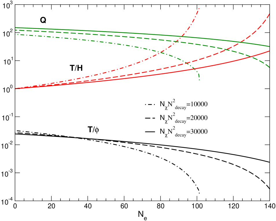
From the approximated expression for the spectral index, Eq. (124), if one wants to keep within the observable range, it requires , which for gives the lower bound . Again, having slow-roll warm inflation for example with needs , but for it only requires . As an example, Fig. 7 shows the predicted spectral index depending on the number of e-folds left to the end of inflation, for and . The corresponding spectral index of the primordial spectrum would be that at around 50-55 e-folds, which is always . The value of the running can be obtained from Eq. (125), and it is given respectively by .

Controlling the amplitude for the primordial spectrum from getting too large was found to require values of as large as possible, but not too large values of . For values of , within the range of Eq. (129), the amplitude remains below say for values of of order . Therefore in these kinds of models parameter values can be found giving rise to the right order of magnitude for the primordial spectrum in the strong dissipative regime, but the stronger constraint comes from avoiding an overly blue-tilted spectrum. The results for this example also reveal one generic feature of warm inflation solutions in quantum field theory models, that the total duration of inflation tends to be small, of order the observational requirement of e-folds. This is in contrast to cold inflation models, which in general cases can predict huge numbers of e-folds, orders of magnitude larger that the observational lower bound. This fact about small e-folds in warm inflation has been explored as a possible solution to the low quadrapole observed in the CMB data Berera:1997wz . Moreover, the small e-folds predicted in warm inflation could also be a possible benefit to the transplankian problem, in which small e-folds of inflation are preferred Martin:2000xs ; Niemeyer:2000eh .
Case : Hybrid quartic and higher powers. In this case having 50 e-folds in the strong regime requires for example for , and for . In addition if we want to get the right amplitude for the spectrum and spectral index, it increases by one order of magnitude, since the quartic coupling has to be adjusted to rather small values, and then the initial value of the field to larger values to have . Numbers do not change much whether 10 or 50 e-folds of inflation are demanded in the strong dissipative regime.
VII.3 hilltop potential

In BuenoSanchez:2008nc the warm hilltop model Boubekeur:2005zm was investigated for the potential
where , , and the dots represent higher order terms that become important only after relevant scales exit the horizon during inflation. The inflaton field is coupled to the fields of the two stage mechanism in Eq. (115). The scenario starts with the inflaton field close to the hilltop. In BuenoSanchez:2008nc this model was constrained to obtain adequate e-folds of warm inflation and a consistent amplitude for density perturbations. In addition constraints were placed to avoid gravitino overproduction. The resulting parameter space for the strong dissipative warm inflation regime is shown in Fig. 8, where . Moreover nongaussian effects in warm inflation Gupta:2002kn ; Moss:2007cv ; Chen:2007gd have been studied for this model in BuenoSanchez:2008nc . In the strong dissipative regime, there are in general large nongaussian effects Moss:2007cv ; Chen:2007gd . In particular it was shown in Moss:2007cv that entropy fluctuations during warm inflation play an important role in generating non-Gaussianity, with the prediction
| (130) |
where is the non-linearity parameter and . For the warm inflation results in Fig. 8, ranges from to , and this implies from the above equation that ranges from to . This is an interesting result in light of the recent WMAP analysis: the third year CMB data Yadav:2007yy gives at confidence level, although the five-year WMAP data Komatsu:2008hk give the limit ( CL). The latest data show then a tendency for , although this still will need to be confirmed by future data, and in particular by data from Planck surveyor satellite planck . If this is the case, this would disfavor conventional cold inflation models which generally yield very low values of . On the other hand, the strong dissipative warm inflation regime, such as the one found in this hilltop model, would be consistent with a non-gaussian signal. For example, in this case taking translates in an upper limit on , and therefore from Fig. 8 on a lower limit on the scale of inflation given by GeV.
VIII Conclusions and Future Perspectives
Generically, the inflaton interacts with other fields in any typical inflation model and so its dynamics is dissipative. As such, inflation, like most dynamics in nature is an open system phenomenon, thus requiring a much more complex analysis of its dynamics than the one typically formulated for the cold inflation picture. This general point has been voiced by B. L. Hu and coworkers hu1 and more specifically in the initial motivating papers of warm inflation Berera:1995wh ; Berera:1995ie ; Berera:1996nv ; BGR . In all these cases, the point has been made that the problem of inflation encompasses many different branches of Physics, from nonequilibrium statistical dynamics to particle physics phenomenology.
Warm inflation dynamics is a rich area of study for both quantum field theory real time dynamics and for particle physics model building. The study of the warm inflation dynamics has almost exclusively motivated the understanding of strong dissipative behavior in quantum field theory. This started initially with the work of Berera, Gleiser and Ramos BGR , in which dissipation was examined in the overdamped regime for the first time in quantum field theory using extended linear response calculations. Since then, specific progress has been made to underpin interaction structures in interacting quantum field theory models which lead to strong dissipative behavior under warm inflationary conditions BR1 ; BRplb1 ; BRfrw ; BRplb2 . At a more general level, this work has motivated the first calculations of dissipation in the low temperature regime mx . In this review, a physical picture has also been developed in Sec. V, for explaining the dissipation behavior found in warm inflation from the quantum field theory calculations, and this is further developed in grahammoss .
Up to now all these studies has been based on variants of linear response methods, in which case the dynamics is supposed to happen close to equilibrium, or in a quasi-adiabatic regime, including various types of resummations. Several extensions to this work, which will give a more accurate understanding of dissipation, are under way. For instance, when departing from the quasi-adiabatic regime for the field dynamics, it is expected that the local Markovian approximation commonly used to analyse the field equations can differ significantly from the exact nonlocal equations. Preliminary tests have shown that this difference can be very large for a period of time starting from the initial period, but with differences between the dynamics getting smaller at longer times, depending on the model parameters FRS .
The methods used in this review are all based on the effective equation of motion derived from the action functional. In order to study strong nonequilibrium dynamics, it requires methods beyond these. In this case, full kinetic set of equations for the relevant fields have to be studied, which contain information not only of the inflaton effective dynamics but also about thermalisation and equilibration. Work in this direction, also can help to better understand the physics of particle production during the system dynamics and be used to check the reliability of using the approximation of thermal initial conditions for the bath fields. Initial work in this direction, though not directly related to the type of models relevant to warm inflation as discussed extensively e.g. in Sec. VII, has appeared Aarts:2007ye , while a work more on the warm inflation dynamics motivated side is under way BMR .
This review has presented in detail the methods used so far to understand warm inflation dynamics as well as the limitations of these studies. In particular these methods used so far are primarily quasi-adiabatic approximations for the fields with the assumption of near thermal equilibrium evolution. Despite these limitations, these results find parameter regimes in which physically acceptable solutions exist over time periods sufficiently long to be of use in studies of warm inflation. During this time interval in which these approximations apply, and where a local Markovian dynamics can be used, in contrast to the full non Markovian one, in the typical model implementations discussed in Sec. VII, the amount of radiation production was seen to be sufficient to change the cold inflationary picture predictions regarding the density perturbations, thus requiring its description in terms of the warm inflation picture. Moreover, once dissipative effects are strong enough, inflation can be sustained and driven longer than when these effects are neglected. Consequently, parameter values typically required in the cold inflation case can be relaxed, which can help to evade various problems that plaque the standard scenario of inflation, like the graceful exit and -problem, discussed in details in this review, as well as the problems of quantum-to-classical transition Berera:1995ie ; bel and the initial conditions for inflation BG ; ROR .
The development of the quantum field theory dynamics of warm inflation has in turn been applied to particle physics model building, in which warm inflation dynamics in realised. Early on it was recognisied in Berera:1999ws that warm inflation has some appealing and unique model building features. In particular, it offers a simple solution to the -problem and for monomial potentials, observationally consistent inflation can occur for the inflaton amplitude below the Planck scale . These features have been realised in explicit first principles quantum field theory models of warm inflation in BGR2 ; Berera:1999ws ; bb4 ; BuenoSanchez:2008nc . These studies are now being extended to develop a complete particle cosmology in which not only is warm inflation realised, but in addition other features such as leptogenesis and gravitino abundances are addressed, developing in depth some of the work already started on these topics Taylor:2000jw ; bb1 ; bb4 ; Lambiase:2006md ; BuenoSanchez:2008nc . In a separate direction, the warm inflation models developed so far in bb4 ; BuenoSanchez:2008nc have been in the low temperature regime. In bbrecent this is being extended to higher temperatures. This requires calculating all the thermal loop corrections in the SUSY models that have the two-stage interaction structure Eq. (115) relevant for warm inflation. Some initial work has been done in Hall:2004zr , and a more detailed analysis is now underway bbrecent .
Acknowledgements.
This work was partially supported by a U.K. Particle Physics and Astronomy Research Council (PPARC) Visiting Researcher Grant. In addition A.B. is partially supported by STFC and R.O.R. is partially supported by Conselho Nacional de Desenvolvimento Científico e Tecnológico (CNPq - Brasil) and Fundação de Amparo à Pesquisa do Estado do Rio de Janeiro (FAPERJ).References
- (1) A. H. Guth, Phys. Rev. D 23, 347 (1981);
- (2) A. D. Linde, Phys. Lett. B 108, 389 (1982); A. Albrecht and P. J. Steinhardt, Phys. Rev. Lett. 48, 1220 (1982).
- (3) A. Albrecht, P. J. Steinhardt, M. S. Turner, and F. Wilczek, Phys. Rev. Lett. 48, 1437 (1982); A. D. Dolgov and A. D. Linde, Phys. Lett. B116, 329 (1982); L. F. Abbott, E. Farhi, and M. B. Wise, Phys. Lett. B117, 29 (1982).
- (4) A. Linde, Phys. Lett. B129, 177 (1983).
- (5) L. Z. Fang, Phys. Lett. B 95, 154 (1980).
- (6) I. G. Moss, Phys. Lett. B 154, 120 (1985).
- (7) J. Yokoyama and K. i. Maeda, Phys. Lett. B 207, 31 (1988).
- (8) A. Berera and L. Z. Fang, Phys. Rev. Lett. 74, 1912 (1995).
- (9) A. Berera, Phys. Rev. Lett. 75, 3218 (1995).
- (10) A. Berera, Phys. Rev. D 55, 3346 (1997).
- (11) A. Berera, Nucl. Phys. B 585, 666 (2000).
- (12) A. Berera, Phys. Rev. D 54, 2519 (1996).
- (13) A. Berera, M. Gleiser and R. O. Ramos, Phys. Rev. D58, 123508 (1998).
- (14) J. Yokoyama and A. D. Linde, Phys. Rev. D 60, 083509 (1999).
- (15) A. Berera, M. Gleiser and R. O. Ramos, Phys. Rev. Lett. 83, 264 (1999).
- (16) A. Berera and R. O. Ramos, Phys. Rev. D 63, 103509 (2001).
- (17) I. G. Moss and C. Xiong, hep-ph/0603266.
- (18) A. Berera, Contemp. Phys. 47, 33 (2006).
- (19) Figure 1 taken from Berera:2006xq with permission from the publishers http://www.informaworld.com.
- (20) S. Alexander, R. Brandenberger and J. Magueijo, Phys. Rev. D 67, 081301 (2003).
- (21) J. Magueijo and L. Pogosian, Phys. Rev. D 67, 043518 (2003).
- (22) P. Ferreira and J. Magueijo, arXiv:0708.0429 [astro-ph].
- (23) I. G. Moss and C. Xiong, JCAP 0811, 023 (2008).
- (24) H. P. de Oliveira and R. O. Ramos, Phys. Rev. D57, 741 (1998).
- (25) E. Gunzig, R. Maartens, and A. V. Nesteruk, Class. Quant. Grav. 15, 923 (1998).
- (26) A. Berera, T. W. Kephart and S. D. Wick, Phys. Rev. D 59, 043510 (1999).
- (27) M. Bellini, Phys. Rev. D58, 103518 (1998); Nucl. Phys. 563, 245 (1999); Phys. Rev. D63, 123510 (2001); Phys.Rev.D67:027303,2003.
- (28) W. Lee and L. Z. Fang, Phys. Rev. D59, 083503 (1999).
- (29) J. M. F. Maia, and J. A. S. Lima, Phys. Rev. D60, 101301 (1999); Phys. Rev. D 65, 083513 (2002).
- (30) A. P. Billyard and A. A. Coley, Phys. Rev. D 61, 083503 (2000).
- (31) A. N. Taylor, and A. Berera, Phys. Rev. D 62, 083517 (2000).
- (32) J. F. Donoghue, JHEP 0008 (2000) 022.
- (33) H. P. de Oliveira and S. E. Joras, Phys. Rev. D64, 063513 (2001).
- (34) I. Dymnikova and M. Khlopov, Eur. Phys. J. C 20, 139 (2001).
- (35) L. P. Chimento, A. S. Jakubi, N. A. Zuccala, and D. Pavon, Phys. Rev. D65, 083510 (2002).
- (36) H. P. De Oliveira, Phys. Lett. B 526, 1 (2002).
- (37) R. H. Brandenberger and Y. Yamaguchi, Phys. Rev. D 68, 023505 (2003).
- (38) L. M. H. Hall, I. G. Moss, and A. Berera, Phys. Rev. D 69, 083525 (2004); Phys. Lett. B 589, 1 (2004).
- (39) R. Jeannerot and M. Postma, JHEP 0505, 071 (2005).
- (40) J. P. Mimoso, A. Nunes and D. Pavon, Phys. Rev. D 73, 023502 (2006).
- (41) S. del Campo and R. Herrera, Phys. Lett. B653, 122 (2007); M. A. Cid, S. del Campo and R. Herrera, JCAP 0710, 5 (2007).
- (42) M. Bastero-Gil and A. Berera, Phys. Rev. D 76, 043515 (2007).
- (43) L. M. H. Hall and H. V. Peiris, JCAP 0801, 027 (2008).
- (44) J. C. Bueno Sanchez, M. Bastero-Gil, A. Berera and K. Dimopoulos, Phys. Rev. D 77, 123527 (2008).
- (45) D. Battefeld, T. Battefeld and A. C. Davis, arXiv:0806.1953 [hep-th].
- (46) S. Mohanty and A. Nautiyal, arXiv:0807.0317 [hep-ph].
- (47) C. Panagiotakopoulos, Phys. Rev. D55, 7335 (1997); A. Linde and A. Riotto, Phys. Rev. D56, R1841 (1997); V. N. Senoguz and Q. Shafi, Phys. Lett. B567, 79 (2003).
- (48) E. J. Copeland, A. R. Liddle, D. H. Lyth, E. D. Stewart and D. Wands, Phys. Rev. D 49, 6410 (1994).
- (49) M. Dine, L. Randall and S. Thomas, Phys. Rev. Lett. 75, 398 (1995).
- (50) M. K. Gaillard, H. Murayama and K. A. Olive, Phys. Lett. B 355, 71 (1995).
- (51) C. F. Kolda and J. March-Russell, Phys. Rev. D 60, 023504 (1999).
- (52) N. Arkani-Hamed, H. C. Cheng, P. Creminelli and L. Randall, JCAP 0307, 003 (2003).
- (53) S. C. Davis and M. Postma, JCAP 0804, 022 (2008).
- (54) E. Halyo, Phys. Lett. B 387, 43 (1996).
- (55) P. Binetruy and G. R. Dvali, Phys. Lett. B 388, 241 (1996).
- (56) I. G. Moss and C. Xiong, JCAP 0704, 007 (2007).
- (57) K. Chou, Z. Su, B. Hao and L. Yu, Phys. Rep. 118, 1 (1985).
- (58) An accessible introduction to the real-time formalism can be found in R. Rivers, Path Integral Methods in Quantum Field Theory, Cambridge University Press, (Cambridge 1987).
- (59) N. P. Landsman and Ch. G. van Weert, Phys. Rep. 145, 141 (1987).
- (60) M. Le Bellac, Thermal Field Theory (Cambridge University Press, Cambridge, 1996).
- (61) J. Schwinger, Jour. Math. Phys. (N.Y.) 2, 407 (1961); P. M. Bakshi and K. T. Mahanthappa, Jour. Math. Phys. (N.Y.) 4, 1 (1963); 4, 12 (1963); L. V. Keldysh, Zh. Eksp. Teor. Fiz. 47, 1515 (1964); A. Niemi and G. Semenoff, Ann. Phys. (NY) 152, 105 (1984); Nucl. Phys. B230, 181 (1984).
- (62) O. Eboli, R. Jackiw and S.-Y. Pi, Phys. Rev. D 37, 3557 (1989); M. Samiullah, O. Eboli and S.-Y. Pi, Phys. Rev. D 44, 2335 (1991).
- (63) J. Berges and J. Cox, Phys. Lett. B517, 369 (2001); J. Berges, Nucl. Phys. A699, 847 (2002).
- (64) E. Calzetta and B. L. Hu, Phys. Rev. D 61, 025012 (2000); A. Jakovac, Phys. Rev. D 65, 085029 (2002).
- (65) A. Einstein, The Collected Papers of Albert Einstein, ed. John Stachel et al. , vol. 2, 170-82, 206-22 (1987-).
- (66) A. O. Caldeira and A. J. Leggett, Physica 121A, 587 (1983).
- (67) B. L. Hu, J. P. Paz and Y. Zhang, Phys. Rev. D 47, 1594 (1993).
- (68) A. Hosoya and M. Sakagami, Phys. Rev. D 29, 2228 (1984).
- (69) M. Morikawa and M. Sasaki, Phys. Lett. B165, 59 (1985).
- (70) M. Morikawa, Phys. Rev. D 33, 3607 (1986).
- (71) B. L. Hu, J. P. Paz and Y. Zhang, in The Origin of Structure in the Universe, Ed. E. Gunzig and P. Nardone (Kluwer Acad. Publ. 1993); E. Calzetta and B. L. Hu, Phys. Rev. D 49, 6636 (1994); ibid 52, 6770 (1995); B. L. Hu and A. Matacz, Phys. Rev. D 51, 1577 (1995); A. Matacz, Phys. Rev. D 55, 1860 (1997); S. A. Ramsey and B. L. Hu, Phys. Rev. D 56, 678 (1997), Erratum-ibid. 57, 3798 (1998).
- (72) D. Lee and D. Boyanovsky, Nucl. Phys. B406, 631 (1993).
- (73) D. Boyanovsky, H. J. de Vega, R. Holman, D. -S. Lee and A. Singh, Phys. Rev. D 51, 4419 (1995).
- (74) M. Gleiser and R. O. Ramos, Phys. Rev. D50, 2441 (1994).
- (75) A. Ringwald, Ann. Phys. 177, 129 (1987); Phys. Rev. D36, 2598 (1987)
- (76) D. Boyanovsky, R. Holman and S. P. Kumar, Phys. Rev. D 56, 1958 (1997).
- (77) A. Berera and R. O. Ramos, Phys. Rev. D 71, 023513 (2005).
- (78) J. Yokoyama, Phys. Rev. D70, 103511 (2004).
- (79) A. Berera, I. G. Moss and R. O. Ramos, Phys. Rev. D 76, 083520 (2007).
- (80) I. D. Lawrie, Phys.Rev. D 66, 041702 (2002); ibid. 67, 045006 (2003); ibid. 71, 025021 (2005); J. M. Almeida and I. D. Lawrie, arXiv:0711.3713.
- (81) G. Aarts and A. Tranberg, Phys. Rev. D77, 123521 (2008).
- (82) A. Berera and R. O. Ramos, Phys. Lett. B567, 294 (2003).
- (83) A. Berera and R. O. Ramos, Phys. Lett. B607, 1 (2005).
- (84) I. G. Moss and C. Graham, Phys. Rev. D78, 123526 (2008).
- (85) G. Semenoff and N. Weiss, Phys. Rev. D31, 689 (1985).
- (86) H. Leutwyler and S. Mallik, Ann. Phys. (NY) 205, 1 (1991).
- (87) G. Semenoff and N. Weiss, Phys. Rev. D31, 699 (1985).
- (88) N. D. Birrel and P. C. W. Davis, Quantum Fields in Curved Space (Cambridge University Press, Cambridge, England, 1982); S. A. Fulling, Aspects of Quantum Field Theory in Curved Space Time (Cambridge University Press, Cambridge, England, 1989).
- (89) S. Habib, Phys. Rev. D46, 2408 (1992).
- (90) G. German, G. G. Ross and S. Sarkar, Phys. Lett. B 469, 46 (1999).
- (91) L. Boubekeur and D. H. Lyth, JCAP 0507, 010 (2005).
- (92) G. G. Ross and S. Sarkar, Nucl. Phys. B 461, 597 (1996).
- (93) J. A. Adams, G. G. Ross and S. Sarkar, Phys. Lett. B 391, 271 (1997).
- (94) D. H. Lyth and A. Riotto, Phys. Rept. 314, 1 (1999).
- (95) C. P. Burgess, PoS P2GC, 008 (2006) [Class. Quant. Grav. 24, S795 (2007)].
- (96) L. M. H. Hall and I. G. Moss, Phys. Rev. D 71, 023514 (2005).
- (97) A. Berera and T. W. Kephart, Phys. Lett. B 456, 135 (1999).
- (98) A. Berera and T. W. Kephart, Phys. Rev. Lett. 83, 1084 (1999).
- (99) E. Komatsu et al. [WMAP Collaboration], 0803.0547 [astro-ph].
- (100) A. D. Linde, Phys. Rev. D 49, 748 (1994).
- (101) G. Dvali, Q. Shafi and R. Schaefer, Phys. Rev. Lett 73, 1886 (1994).
- (102) G. Lazarides, R. K. Schaefer and Q. Shafi, Phys. Rev. D56, 1324 (1997).
- (103) M. Bastero-Gil, S. F. King and Q. Shafi, Phys. Lett. B 651, 345 (2007).
- (104) J. Bagger and E. Poppitz, Phys. Rev. Lett. 71, 2380 (1993).
- (105) L. Boubekeur and G. Tasinato, Phys. Lett. B 524, 342 (2002).
- (106) H. P. Nilles and N. Polonsky, Phys. Lett. B 412, 69 (1997).
- (107) C. F. Kolda and N. Polonsky, Phys. Lett. B 433, 323 (1998).
- (108) R. A. Battye, B. Garbrecht and A. Moss, JCAP 0609, 007 (2006).
- (109) M. Bastero-Gil and A. Berera, Phys. Rev. D 71, 063515 (2005).
- (110) A. Berera, L. Z. Fang and G. Hinshaw, Phys. Rev. D 57, 2207 (1998); A. Berera and A. F. Heavens, Phys. Rev. D 62, 123513 (2000).
- (111) J. Martin and R. H. Brandenberger, Phys. Rev. D 63, 123501 (2001).
- (112) J. C. Niemeyer, Phys. Rev. D 63, 123502 (2001).
- (113) S. Gupta, A. Berera, A. F. Heavens and S. Matarrese, Phys. Rev. D 66, 043510 (2002).
- (114) B. Chen, Y. Wang and W. Xue, JCAP 0805, 014 (2008).
- (115) A. P. S. Yadav and B. D. Wandelt, Phys. Rev. Lett. 100, 181301 (2008).
-
(116)
Planck Surveyor Mission:
http://www.rssd.esa.int/Planck. - (117) R. S. Farias, R. O. Ramos and A. L. da Silva, Braz. J. Phys. 38, 499 (2008).
- (118) A. Berera, I. G. Moss and R. O. Ramos, work in progress (2009).
- (119) M. Bellini, Phys. Lett. B 428, 31 (1998).
- (120) A. Berera and C. Gordon, Phys. Rev. D 63, 063505 (2001).
- (121) R. O. Ramos, Phys. Rev. D 64, 123510 (2001).
- (122) A. N. Taylor and A. R. Liddle, Phys. Rev. D 64, 023513 (2001).
- (123) G. Lambiase and S. Mohanty, JCAP 0712, 008 (2007).
- (124) M. Bastero-Gil and A. Berera, work in progress (2009).