Computing with almost periodic functions

R.V. Moody M. Nesterenko  and  J. Patera
Abstract.

The paper develops a method for discrete computational Fourier analysis of functions defined on quasicrystals and other almost periodic sets. A key point is to build the analysis around the emerging theory of quasicrystals and diffraction in the setting on local hulls and dynamical systems. Numerically computed approximations arising in this way are built out of the Fourier module of the quasicrystal in question, and approximate their target functions uniformly on the entire infinite space.

The methods are entirely group theoretical, being based on finite groups and their duals, and they are practical and computable. Examples of functions based on the standard Fibonacci quasicrystal serve to illustrate the method (which is applicable to all quasicrystals modeled on the cut and project formalism).

1. Introduction

In this paper we consider the problem of discrete methods for dealing with functions that are intrinsically almost periodic, but not actually periodic. Quasicrystals, quasicrystalline photonic crystals, Faraday wave experiments, and other physical phenomena arising from the interaction of incommensurate frequencies, all display the features of almost periodicity. As a typical example one may think of a potential field of a physical quasicrystal. The salient features of quasicrystals are highly structured long-range order (represented by pure point or near pure point diffraction) but no periodic order. Thus the potential is not a periodic function, but rather belongs to the domain of almost periodic functions.

Here we put forth a method for finite discrete analysis of almost periodic functions that has the following main features:

  • It is entirely based on group theoretical methods, primarily finite groups and their duals.

  • The discretely computed Fourier approximants are themselves almost periodic and uniformly approximate their target functions over their entire domains.

  • The Fourier frequencies involved in the approximation lie in the module of Fourier frequencies of the target function.

A standard approach to modeling such structures is to take a finite part of it, impose periodic boundary conditions, rationalize and reduce the object to a periodic approximant, and then apply usual crystallography. Although this type of periodization is used routinely and successfully for many modelling problems in the theory of quasicrystals, it is not entirely satisfactory. Almost periodic order goes beyond periodic order in fundamental ways, its essence appearing as a underlying incommensurability which pervades every part of the theory. For instance, a key feature of quasicrystals appears in the Fourier module which parameterizes the Bragg spectrum and always has rank higher than (typically double) the dimension of the ambient space of the quasicrystal. Periodization destroys this, and by its nature can only produce results that can fit data over the finite range specified by the imposed periodization boundaries, whereas the essence of the material is that its order is long-range. The present paper does not involve any periodization and avoids these issues.

The theory of almost periodic functions was initiated by H. Bohr [7], on the basis of earlier work on uniform approximation of functions by trigonometric polynomials by P. Bohl. It was greatly extended by the work of A. Besicovitch [3], S. Bochner, J. von Neumann, [4, 5, 6], N. Wiener [24], H. Weyl [23], and others [9, 15, 1]. The advent of quasicrystals and aperiodic tilings instigated a revival of the field, and led to extensive study of the cut and project formalism and the theory of pure point diffraction [16, 17, 11, 22] which have become the mainstays of experimentalists and theorists alike. An important component of this is the use of dynamical systems and dynamical hulls. These are ideally suited to the phenomenon of almost periodicity, which appears in the dynamics as recurrence, and provide a natural setting for the Fourier analysis that is used to study it.

Although our study is of almost periodic functions, their importance in the subject of quasicrystals is that they arise from functions whose behaviour is dominated by the local environments of the quasicrystal in question. The way in which this happens is mostly taken for granted, but in fact there are some interesting assumptions involved, and for this reason we begin by formally defining local functions with respect to a given point set ΛΛ\Lambda, and showing how it is that they are connected with almost periodic functions.

We can create a dynamical hull (X,μ)𝑋𝜇(X,\mu) from ΛΛ\Lambda. This is a compact space that arises from ΛΛ\Lambda and its translations, and it lies at the heart of the Fourier analysis of local functions on ΛΛ\Lambda. One assumes (in many important cases it is forced) a probability measure μ𝜇\mu on which dsuperscript𝑑\mathbb{R}^{d} acts in a measure preserving way. A local function f𝑓f lifts to some new function F𝐹F on (X,μ)𝑋𝜇(X,\mu), and this is an L2superscript𝐿2L^{2} function. Now the analysis of f𝑓f can be related directly to the analysis of F𝐹F, and for this we have a powerful tool in the form of the action of dsuperscript𝑑\mathbb{R}^{d} on L2(X,μ)superscript𝐿2𝑋𝜇L^{2}(X,\mu), which is unitary. All of this material is explained in §2.

To go further, we next place ourselves in the situation of the cut and project formalism, which is the standard method of modeling used in the study of quasicrystals. The set ΛΛ\Lambda is now assumed to be a model set (cut and project set). In this setting the hull (X,μ)𝑋𝜇(X,\mu), and more particularly L2(X,μ)superscript𝐿2𝑋𝜇L^{2}(X,\mu), can be described explicitly in terms of a higher dimensional torus111More generally a compact Abelian group(higher dimensional periodicity!), and it is a straightforward matter to carry out Fourier analysis of F𝐹F. It is the restriction of this Fourier analysis back to f𝑓f that provides the required Fourier analysis of f𝑓f. By its very nature this is almost periodic and captures the full aperiodic nature of ΛΛ\Lambda, including the correct Fourier module in which physical information actually appears. This is the content of §3. Readers familiar with the cut and project method who do not wish to go through the theory of local hulls and local functions may read §3.1 and §3.4, and then continue starting at §4.

This theoretical analysis is based on higher dimensional structures that are not explicitly computatable, as well as the usual array of countably many Fourier coefficients, each of which is the outcome of integration. To be a practical tool, the analysis has to be reduced to finitely many objects that are explicitly computable entirely in the context of the given function f𝑓f. The resulting approximants are trigonometric polynomials (quasi-periodic functions) whose frequencies come from the Fourier module of the original function. In §4 we outline the method of discretization, which depends primarily on the construction of a refinement lattice of the lattice of the cut and project scheme and, along with it, its dual lattice. Together these produce two finite groups which are in \mathbb{Z}-duality to each other. The selection of data points and appropriate Fourier frequencies is governed by these two groups.

This is best illustrated by examples and for this we have chosen two local functions based on one of the famous Fibonacci point sets. This has the advantage of being straightforward to construct and easy to visualize, while at the same time containing all the essential features of more general model sets. §5 prepares the mathematics of the Fibonacci cut and project scheme, and §6 shows some explicit computations for the particular local functions we have chosen. As is evident from the examples, the main effort required is in the creation of the data points. Once this is done, the same set of data points and Fourier frequencies will work for any almost periodic function arising from the same cut and project scheme.

The results are striking in two ways. First of all, the approximating functions are remarkably good, given the amount of data from which they are produced. Second, the approximating functions are not just local approximations they are also global approximations, in the sense that they provide finite Fourier series that approximate f𝑓f throughout its entire domain (namely \mathbb{R}). Of course this was to be expected, but it is impressive to see it in action.

The numerical methods we introduce here are designed to be efficient and, of course, to utilize the inherent almost periodicity. In the development of the theory we provide error estimates that can be worked out specifically in the cases of interest. We note that the primary weakness in the error estimates is not one that is due to the aperiodic nature of the problem, but one that always appears in Fourier analysis, namely how well can one approximate a function if one uses only finitely many of its Fourier coefficients.


2. Continuous functions on aperiodic point sets

2.1. Local hulls

We work in dsuperscript𝑑\mathbb{R}^{d}, a real Euclidean space of finite dimension d𝑑d. For r>0𝑟0r>0, let Dr(d)subscript𝐷𝑟superscript𝑑D_{r}(\mathbb{R}^{d}), be all point sets ΛdΛsuperscript𝑑\Lambda\subset\mathbb{R}^{d} for which the distance |xy|r𝑥𝑦𝑟|x-y|\geq r for all x,yΛ𝑥𝑦Λx,y\in\Lambda. This means that Drsubscript𝐷𝑟D_{r} consists of all discrete point sets with minimal separation rabsent𝑟\geq r between their points.

The local topology on Dr(d)subscript𝐷𝑟superscript𝑑D_{r}(\mathbb{R}^{d}) can be intuitively introduced as follows. Two sets Λ1subscriptΛ1\Lambda_{1} and Λ2subscriptΛ2\Lambda_{2} of Dr(d)subscript𝐷𝑟superscript𝑑D_{r}(\mathbb{R}^{d}) are ‘close’ if, for some large R𝑅R and some small ϵitalic-ϵ\epsilon, one has

Λ1BRsubscriptΛ1subscript𝐵𝑅\displaystyle\Lambda_{1}\cap B_{R} Λ2+Bϵ,absentsubscriptΛ2subscript𝐵italic-ϵ\displaystyle\subset\ \Lambda_{2}+B_{\epsilon}\,, (1)
Λ2BRsubscriptΛ2subscript𝐵𝑅\displaystyle\Lambda_{2}\cap B_{R} Λ1+Bϵ,absentsubscriptΛ1subscript𝐵italic-ϵ\displaystyle\subset\ \Lambda_{1}+B_{\epsilon}\,,

where BRsubscript𝐵𝑅B_{R} (resp. Bϵsubscript𝐵italic-ϵB_{\epsilon}) is the ball of radius R𝑅R (resp. ϵitalic-ϵ\epsilon) around 00. Thus for each point of Λ1subscriptΛ1\Lambda_{1} within the ball BRsubscript𝐵𝑅B_{R}, there is a point of Λ2subscriptΛ2\Lambda_{2} within the distance ϵitalic-ϵ\epsilon of that point; and vice versa. Pairs (Λ1,Λ2)subscriptΛ1subscriptΛ2(\Lambda_{1},\Lambda_{2}) satisfying (1) are called (R,ϵ)𝑅italic-ϵ(R,\epsilon)-close.

Refer to caption
Figure 1. Two sets Λ1subscriptΛ1\Lambda_{1} and Λ2subscriptΛ2\Lambda_{2} of Dr(d)subscript𝐷𝑟superscript𝑑D_{r}(\mathbb{R}^{d}) that are close.

The local topology is actually a metric topology, although we make no use of this fact here.

Definition 1.

For ΛDr(d)Λsubscript𝐷𝑟superscript𝑑\Lambda\in D_{r}(\mathbb{R}^{d}) the local hull of ΛΛ\Lambda is

X(Λ)={t+Λ:td}¯Dr(d),𝑋Λ¯conditional-set𝑡Λ𝑡superscript𝑑subscript𝐷𝑟superscript𝑑X(\Lambda)=\overline{\{t+\Lambda\ :\ t\in\mathbb{R}^{d}\}}\subset D_{r}(\mathbb{R}^{d})\,, (2)

i.e. take all translates of ΛΛ\Lambda and take their closure in the local topology.

Proposition 2.1.

[21] The translation action of dsuperscript𝑑\mathbb{R}^{d} on ΛΛ\Lambda lifts to a translation action on X(Λ)𝑋ΛX(\Lambda). The local hull X(Λ)𝑋ΛX(\Lambda) is compact and the dsuperscript𝑑\mathbb{R}^{d}-action on it is continuous. ∎

Example 1.

Let ΛΛ\Lambda be the lattice dsuperscript𝑑\mathbb{Z}^{d} in dsuperscript𝑑\mathbb{R}^{d}. Then X(Λ)=d/d𝑋Λsuperscript𝑑superscript𝑑X(\Lambda)=\mathbb{R}^{d}/\mathbb{Z}^{d} is the d𝑑d-torus (with its usual topology). Intuitively we translate the lattice around with dsuperscript𝑑\mathbb{R}^{d}. But translation by an element of dsuperscript𝑑\mathbb{Z}^{d} leaves ΛΛ\Lambda invariant. So d/dsuperscript𝑑superscript𝑑\mathbb{R}^{d}/\mathbb{Z}^{d} parameterizes all distinct positions of ΛΛ\Lambda under translation.

Example 2.

Let ΛΛ\Lambda be any Penrose tiling. Then X(Λ)𝑋ΛX(\Lambda) is the set of all Penrose tilings that are locally indistinguishable from some translate of ΛΛ\Lambda. X(Λ)𝑋ΛX(\Lambda) contains considerably more than just the translations of ΛΛ\Lambda. In fact X(Λ)𝑋ΛX(\Lambda) consists of all Penrose tilings based on the same pair of Penrose rhombs and the same orientations as appearing in ΛΛ\Lambda.

Generally one may think of X(Λ)𝑋ΛX(\Lambda) as some sort of local indistinguishability class of ΛΛ\Lambda.

2.2. Continuous functions on X(Λ)𝑋ΛX(\Lambda)

We assume that ΛDr(d)Λsubscript𝐷𝑟superscript𝑑\Lambda\subset D_{r}(\mathbb{R}^{d}) and X(Λ)𝑋ΛX(\Lambda) are as in §2.1.

Consider a function

F:X(Λ).:𝐹𝑋ΛF:X(\Lambda)\ \longrightarrow\ \mathbb{C}\,. (3)

We can define from it a function

f:d.:𝑓superscript𝑑\displaystyle f:\mathbb{R}^{d}\longrightarrow\ \mathbb{C}\,.

by

f(t)=F(t+Λ).𝑓𝑡𝐹𝑡Λf(t)=F(t+\Lambda)\,. (4)

If F𝐹F is continuous then we note that for all t1,t2dsubscript𝑡1subscript𝑡2superscript𝑑t_{1},t_{2}\in\mathbb{R}^{d},

t1+Λ,subscript𝑡1Λ\displaystyle t_{1}+\Lambda, t2+Λare closesubscript𝑡2Λare close\displaystyle\ t_{2}+\Lambda\quad\text{are close}
F(t1+Λ),F(t2+Λ)are close𝐹subscript𝑡1Λ𝐹subscript𝑡2Λare close\displaystyle\Longrightarrow\quad F(t_{1}+\Lambda),\ F(t_{2}+\Lambda)\quad\text{are close}
f(t1),f(t2)are close.𝑓subscript𝑡1𝑓subscript𝑡2are close\displaystyle\Longrightarrow\quad f(t_{1}),\ f(t_{2})\quad\text{are close}\,.

Thus continuity of F𝐹F implies continuity of f𝑓f, and we see that f𝑓f is local, or almost periodic, with respect to ΛΛ\Lambda in the following sense:

Definition 2.

A function f:d:𝑓superscript𝑑f:\mathbb{R}^{d}\ \longrightarrow\ \mathbb{C}  is called local with respect to a set ΛDr(d)Λsubscript𝐷𝑟superscript𝑑\Lambda\in D_{r}(\mathbb{R}^{d}), or ΛΛ\Lambda-local, if for all ϵ>0superscriptitalic-ϵ0\epsilon^{\prime}>0 there exist R𝑅R and ϵitalic-ϵ\epsilon so that whenever t1,t2dsubscript𝑡1subscript𝑡2superscript𝑑t_{1},t_{2}\in\mathbb{R}^{d} satisfy that t1+Λsubscript𝑡1Λt_{1}+\Lambda and t2+Λsubscript𝑡2Λt_{2}+\Lambda are (R,ϵ)𝑅italic-ϵ(R,\epsilon)-close then

|f(t1)f(t2)|<ϵ.𝑓subscript𝑡1𝑓subscript𝑡2superscriptitalic-ϵ\displaystyle|f(t_{1})-f(t_{2})|<\epsilon^{\prime}\,.

The intuitive meaning of this is that f𝑓f has the very natural property, at least from the perspective of physical systems, that it looks very much the same at places where the local environment looks the same. Local functions are easily seen to be continuous on dsuperscript𝑑\mathbb{R}^{d}.

Using locality, we can go in the opposite direction. Let ΛDr(d)Λsubscript𝐷𝑟superscript𝑑\Lambda\in D_{r}(\mathbb{R}^{d}) and let f:d:𝑓superscript𝑑f:\mathbb{R}^{d}\ \rightarrow\ \mathbb{C} be local with respect to ΛΛ\Lambda. Define

F:{t+Λ:td}:𝐹conditional-set𝑡Λ𝑡superscript𝑑\displaystyle F:\{t+\Lambda\ :\ t\in\mathbb{R}^{d}\}\ \longrightarrow\ \mathbb{C}

(so that F𝐹F is a function on a part of Dr(d)subscript𝐷𝑟superscript𝑑D_{r}(\mathbb{R}^{d})) by

F(t+Λ)=f(t).𝐹𝑡Λ𝑓𝑡\displaystyle F(t+\Lambda)=f(t)\,.

Then F𝐹F is continuous on {t+Λ:td}conditional-set𝑡Λ𝑡superscript𝑑\{t+\Lambda\ :\ t\in\mathbb{R}^{d}\} with respect to the local topology. In fact it is uniformly continuous. The reason for this is that the continuity condition which defines the local-ness of f𝑓f is based on the uniformity (i.e. the notion of (R,ϵ)𝑅italic-ϵ(R,\epsilon)-closeness) defining the local topology of {t+Λ:td}conditional-set𝑡Λ𝑡superscript𝑑\{t+\Lambda\ :\ t\in\mathbb{R}^{d}\}.

It follows that F𝐹F lifts uniquely to a continuous function (3) on the local hull X(Λ)𝑋ΛX(\Lambda).

Proposition 2.2.

For each local function f𝑓f with respect to ΛΛ\Lambda there is a unique continuous function (3) on the local hull, whose restriction to the orbit of ΛΛ\Lambda is f𝑓f. Every continuous function on the local hull of ΛΛ\Lambda arises in this way. ∎

Thus we see that a locality with respect to ΛΛ\Lambda and the existence and continuity of an extension function on X(Λ)𝑋ΛX(\Lambda) amount to the same thing.

In the situation that X(Λ)𝑋ΛX(\Lambda) is equipped with an dsuperscript𝑑\mathbb{R}^{d}-invariant probability measure μ𝜇\mu (i.e. a positive Borel measure μ𝜇\mu with μ(t+A)=μ(A)𝜇𝑡𝐴𝜇𝐴\mu(t+A)=\mu(A) for all Borel sets and with μ(X(Λ))=1𝜇𝑋Λ1\mu(X(\Lambda))=1), the action of dsuperscript𝑑\mathbb{R}^{d} on X(Λ)𝑋ΛX(\Lambda) leads to unitary action T𝑇T of dsuperscript𝑑\mathbb{R}^{d} on L2(X(Λ),μ)superscript𝐿2𝑋Λ𝜇L^{2}(X(\Lambda),\mu). Namely for all FL2(X(Λ),μ)𝐹superscript𝐿2𝑋Λ𝜇F\in L^{2}(X(\Lambda),\mu) and for all td𝑡superscript𝑑t\in\mathbb{R}^{d}, TtFsubscript𝑇𝑡𝐹T_{t}F is the function defined by TtF(Γ)=F(t+Γ)subscript𝑇𝑡𝐹Γ𝐹𝑡ΓT_{t}F(\Gamma)=F(-t+\Gamma) and with

FG:=X(Λ)FG¯𝑑μassigninner-product𝐹𝐺subscript𝑋Λ𝐹¯𝐺differential-d𝜇\displaystyle\langle F\mid G\rangle:=\int_{X(\Lambda)}F\overline{G}\,d\mu

we have

TtFTtG=FG.inner-productsubscript𝑇𝑡𝐹subscript𝑇𝑡𝐺inner-product𝐹𝐺\displaystyle\langle T_{t}F\mid T_{t}G\rangle=\langle F\mid G\rangle\,.

In principle the spectral theory of L2(X(Λ),μ)superscript𝐿2𝑋Λ𝜇L^{2}(X(\Lambda),\mu) should allow one analyze ΛΛ\Lambda-local functions f:d:𝑓superscript𝑑f:\mathbb{R}^{d}\rightarrow\mathbb{C} by analyzing their corresponding functions F𝐹F on L2(X(Λ),μ)superscript𝐿2𝑋Λ𝜇L^{2}(X(\Lambda),\mu).

For one very important class of subsets ΛΛ\Lambda this can actually be carried out in detail – namely the class of model sets, which we now introduce.

3. Local functions on model sets

3.1. Cut and project schemes, model sets and torus parametrization

An important class of point sets ΛdΛsuperscript𝑑\Lambda\subset\mathbb{R}^{d} for which we know a considerable amount about the corresponding hulls X(Λ)𝑋ΛX(\Lambda) is the class of cut and project sets, or the model sets as they are often called [16, 17].

Consider the cut and project scheme

dsuperscript𝑑\displaystyle\mathbb{R}^{d}\ ||\displaystyle\overset{||}{\longleftarrow}\quad dsuperscript𝑑\displaystyle\mathbb{R}^{d} ×dabsentsuperscript𝑑\displaystyle\times\mathbb{R}^{d} dperpendicular-tosuperscript𝑑\displaystyle\overset{\perp}{\longrightarrow}\quad\mathbb{R}^{d}
\displaystyle\cup (5)
1111\displaystyle\overset{1-1}{\longleftarrow} L~~𝐿\displaystyle\widetilde{L} dense imagedense image\displaystyle\overset{\text{dense image}}{\longrightarrow}\quad

and a window ΩΩ\Omega. Here L~~𝐿\widetilde{L} is a lattice in d×dsuperscript𝑑superscript𝑑\mathbb{R}^{d}\times\mathbb{R}^{d} which is oriented so that the projections into dsuperscript𝑑\mathbb{R}^{d} are 11111-1 and dense respectively.

In (3.1) the left-hand dsuperscript𝑑\mathbb{R}^{d} is physical space, the space in which ΛΛ\Lambda is going to lie. The right-hand dsuperscript𝑑\mathbb{R}^{d} is internal space, the one that will be used to control the projection of the lattice L~~𝐿\widetilde{L} into physical space. The image of L~~𝐿\widetilde{L} under projection into physical space is denoted by L𝐿L. Since this projection is one-one, LL~similar-to-or-equals𝐿~𝐿L\simeq\widetilde{L} as groups, so L𝐿L is a free Abelian group of rank 2d2𝑑2d, i.e. it has a \mathbb{Z}-basis of 2d2𝑑2d elements. However, it necessarily has accumulation points, and the typical situation is that L𝐿L is dense in physical space.

It is convenient to use notation like x~,x,x~𝑥𝑥superscript𝑥\tilde{x},x,x^{\prime} for the elements of L~~𝐿\widetilde{L} and their respective left and right projections. Then x~=(x,x)~𝑥𝑥superscript𝑥\tilde{x}=(x,x^{\prime}) where x𝑥x runs through L𝐿L. This implies existence of the mapping ():LL:superscript𝐿superscript𝐿(\,\cdot\,)^{\prime}\ :\ L\rightarrow L^{\prime} defined by xxmaps-to𝑥superscript𝑥x\mapsto x^{\prime}, which passes from physical to internal space.

Note that this mapping ()superscript(\,\cdot\,)^{\prime}, as given, is only defined on L𝐿L. It cannot be extended in any canonical way to a mapping ddsuperscript𝑑superscript𝑑\mathbb{R}^{d}\rightarrow\mathbb{R}^{d}. However it does extend canonically to the rational spans of the objects in question, and we shall make use of this later.

We choose a subset ΩΩ\Omega in internal space. This window is assumed to be compact, equal to the closure of its interior, and to have boundary of measure 0. Using it we define

Λ=Λ(Ω)={x:x~L~,xΩ}.ΛΛΩconditional-set𝑥formulae-sequence~𝑥~𝐿superscript𝑥Ω\Lambda=\Lambda(\Omega)=\{x:\tilde{x}\in\widetilde{L},\,x^{\prime}\in\Omega\}\,. (6)

Sets of the form t+Λ(Ω)𝑡ΛΩt+\Lambda(\Omega), td𝑡superscript𝑑t\in\mathbb{R}^{d}, are called cut and project sets or model sets 222Model sets can be taken more generally with any locally compact Abelian group as the internal space.. In particular, for each (x,y)d×d𝑥𝑦superscript𝑑superscript𝑑(x,y)\in\mathbb{R}^{d}\times\mathbb{R}^{d} we may define

Λ(x,y)=x+Λ(y+Ω).subscriptΛ𝑥𝑦𝑥Λ𝑦Ω\Lambda_{(x,y)}=x+\Lambda(-y+\Omega)\,. (7)

If (x,y)(x,y)modL~𝑥𝑦modulosuperscript𝑥superscript𝑦~𝐿(x,y)\equiv(x^{\prime},y^{\prime})\mod\widetilde{L}, then x+Λ(y+Ω)=x+Λ(y+Ω)𝑥Λ𝑦Ωsuperscript𝑥Λsuperscript𝑦Ωx+\Lambda(-y+\Omega)=x^{\prime}+\Lambda(-y^{\prime}+\Omega), as can be verified directly from the definitions. Thus these model sets are parameterized by the torus of dimension 2d2𝑑2d,

(d×d)/L~(/)d=:𝕋.(\mathbb{R}^{d}\times\mathbb{R}^{d})/\widetilde{L}\simeq(\mathbb{R}/\mathbb{Z})^{d}=:\mathbb{T}\,. (8)

We note, though, that the parametrization need not necessarily be 11111-1, i.e. in general, Λ(x,y)=Λ(x,y)(x,y)=(x,y)modL~subscriptΛ𝑥𝑦subscriptΛsuperscript𝑥superscript𝑦𝑥𝑦modulosuperscript𝑥superscript𝑦~𝐿\Lambda_{(x,y)}=\Lambda_{(x^{\prime},y^{\prime})}\nRightarrow(x,y)=(x^{\prime},y^{\prime})\mod\widetilde{L}. In the sequel, for simplicity, we shall usually write (x,y)Lsubscript𝑥𝑦𝐿(x,y)_{L} for the congruence class (x,y)modL~.modulo𝑥𝑦~𝐿(x,y)\mod\widetilde{L}.

There is a natural measure, the Haar measure, θ𝕋subscript𝜃𝕋\theta_{\mathbb{T}} on 𝕋𝕋\mathbb{T}. This measure is the obvious ‘area’ measure in the case of 𝕋2superscript𝕋2\mathbb{T}^{2}, and ‘length’ measure for 𝕋1superscript𝕋1\mathbb{T}^{1}. It is invariant under the dsuperscript𝑑\mathbb{R}^{d}-action: dsuperscript𝑑\mathbb{R}^{d} acts on 2d/L~superscript2𝑑~𝐿\mathbb{R}^{2d}/\widetilde{L} by

t+(x,y)L=(t+x,y)L.𝑡subscript𝑥𝑦𝐿subscript𝑡𝑥𝑦𝐿t+(x,y)_{L}=(t+x,y)_{L}\,. (9)

Of particular importance to us is natural embedding (see Fig. 2.)

d𝕋t(t,0)L,formulae-sequencesuperscript𝑑𝕋maps-to𝑡subscript𝑡0𝐿\mathbb{R}^{d}\,\longrightarrow\,\mathbb{T}\quad\quad t\mapsto(t,0)_{L}\,, (10)

which lies behind the connection between almost periodicity in physical space and periodicity in some higher dimensional setting. The image of this mapping is easily established to be dense in 𝕋𝕋\mathbb{T}.

Now start with Λ=Λ(0,0)=Λ(Ω)ΛsubscriptΛ00ΛΩ\Lambda=\Lambda_{(0,0)}=\Lambda(\Omega), and translate it by elements td𝑡superscript𝑑t\in\mathbb{R}^{d}:

t+Λ(Ω)=t+Λ(0+Ω)=Λ(t,0).𝑡ΛΩ𝑡Λ0ΩsubscriptΛ𝑡0t+\Lambda(\Omega)=t+\Lambda(0+\Omega)=\Lambda_{(t,0)}\,. (11)

Form the local hull X(Λ)𝑋ΛX(\Lambda), the closure of the set of all translates Λ(t,0)subscriptΛ𝑡0\Lambda_{(t,0)} of ΛΛ\Lambda under the local topology (2).

Proposition 3.1.

[22] There is a continuous mapping,

β:X(Λ)𝕋,:𝛽𝑋Λ𝕋\beta:X(\Lambda)\ \longrightarrow\ \mathbb{T}\,, (12)

called the torus parametrization, such that

  • 1)

    β𝛽\beta is onto;

  • 2)

    β𝛽\beta is 1 - 1 almost everywhere, seen from the perspective of Haar measure on 𝕋𝕋\mathbb{T};

  • 3)

    for all td𝑡superscript𝑑t\in\mathbb{R}^{d}, for all ΛX(Λ)superscriptΛ𝑋Λ\Lambda^{\prime}\in X(\Lambda), one has β(t+Λ)=t+β(Λ)𝛽𝑡superscriptΛ𝑡𝛽superscriptΛ\beta(t+\Lambda^{\prime})=t+\beta(\Lambda^{\prime}).

  • 4)

    β(t+Λ)=(t,0)L𝛽𝑡Λsubscript𝑡0𝐿\beta(t+\Lambda)=(t,0)_{L} for all td𝑡superscript𝑑t\in\mathbb{R}^{d}. ∎

X(Λ)𝑋ΛX(\Lambda) and 𝕋𝕋\mathbb{T} are both compact spaces with natural dsuperscript𝑑\mathbb{R}^{d} action, and β:X(Λ)𝕋:𝛽𝑋Λ𝕋\beta:X(\Lambda)\rightarrow\mathbb{T} is an onto dsuperscript𝑑\mathbb{R}^{d} mapping. But X(Λ)𝑋ΛX(\Lambda) and 𝕋𝕋\mathbb{T} are subtly different. Although t+ΛX(Λ)𝑡Λ𝑋Λt+\Lambda\in X(\Lambda) and t+ΛΛ(t,0)maps-to𝑡ΛsubscriptΛ𝑡0t+\Lambda\mapsto\Lambda_{(t,0)} for all t𝑡t, not every element of X(Λ)𝑋ΛX(\Lambda) is a Λ(x,y)subscriptΛ𝑥𝑦\Lambda_{(x,y)} for some (x,y)𝑥𝑦(x,y). Rather, when (y+Ω)L𝑦Ωsuperscript𝐿(-y+\partial\Omega)\cap L^{\prime}\neq\emptyset, then for all xd𝑥superscript𝑑x\in\mathbb{R}^{d} there are always Λ1Λ2subscriptΛ1subscriptΛ2\Lambda_{1}\neq\Lambda_{2} of elements of X(Λ)𝑋ΛX(\Lambda) that are mapped by β𝛽\beta to the same (x,y)Lsubscript𝑥𝑦𝐿(x,y)_{L}. When z~=(z,z)L~~𝑧𝑧superscript𝑧~𝐿\tilde{z}=(z,z^{\prime})\in\widetilde{L} with z(y+Ω)superscript𝑧𝑦Ωz^{\prime}\in(-y+\partial\Omega) then there will always be Λ1,Λ2X(Λ)subscriptΛ1subscriptΛ2𝑋Λ\Lambda_{1},\Lambda_{2}\in X(\Lambda) with β(X(Λ1))=β(X(Λ2))=(x,y)L𝛽𝑋subscriptΛ1𝛽𝑋subscriptΛ2subscript𝑥𝑦𝐿\beta(X(\Lambda_{1}))=\beta(X(\Lambda_{2}))=(x,y)_{L}, yet x+zΛ1,𝑥𝑧subscriptΛ1x+z\in\Lambda_{1}, x+zΛ2𝑥𝑧subscriptΛ2x+z\notin\Lambda_{2}. In other words, there are ambiguities regarding the lattice points that project onto the boundary ΩΩ\partial\Omega of ΩΩ\Omega. An example of this is shown in the footnote appearing in §5.3. The fact that β𝛽\beta is 11111-1 almost everywhere is due to our assumption that the boundary of ΩΩ\Omega has measure 0.

When we say that β𝛽\beta is 1 - 1 almost everywhere, we mean that the set A𝐴A of points ξ𝜉\xi in 𝕋𝕋\mathbb{T}, for which there is more than one point set over ξ𝜉\xi, satisfies θ𝕋(A)=0subscript𝜃𝕋𝐴0\theta_{\mathbb{T}}(A)=0.

There is a unique dsuperscript𝑑\mathbb{R}^{d}-invariant ergodic measure μ𝜇\mu on X(Λ)𝑋ΛX(\Lambda) with μ(X(Λ))=1𝜇𝑋Λ1\mu(X(\Lambda))=1. In fact β𝛽\beta relates μ𝜇\mu and θ𝜃\theta:

β(μ)=θ.𝛽𝜇𝜃\beta(\mu)=\theta\,. (13)

Or more specifically, θ(A)=μ(β1A)𝜃𝐴𝜇superscript𝛽1𝐴\theta(A)=\mu(\beta^{-1}A) for all measurable subsets A𝐴A of 𝕋𝕋\mathbb{T}. With μ𝜇\mu in hand, we can introduce the space L2(X(Λ),μ)superscript𝐿2𝑋Λ𝜇L^{2}(X(\Lambda),\mu) of square integrable functions on X(Λ)𝑋ΛX(\Lambda). As already pointed out, the natural action of dsuperscript𝑑\mathbb{R}^{d} on this is unitary.

3.2. From hulls to tori

Square integrable functions on X(Λ)𝑋ΛX(\Lambda) and square integrable functions on 𝕋𝕋\mathbb{T} can be identified,

L2(X(Λ),μ)L2(𝕋,θ).similar-to-or-equalssuperscript𝐿2𝑋Λ𝜇superscript𝐿2𝕋𝜃L^{2}(X(\Lambda),\mu)\simeq L^{2}(\mathbb{T},\theta)\,. (14)

The isomorphism is easy to understand:

X(Λ)𝑋Λ\textstyle{X(\Lambda)\ignorespaces\ignorespaces\ignorespaces\ignorespaces\ignorespaces\ignorespaces\ignorespaces\ignorespaces}β𝛽\scriptstyle{\beta}Gβ𝐺𝛽\scriptstyle{G\circ\beta}𝕋𝕋\textstyle{\mathbb{T}\ignorespaces\ignorespaces\ignorespaces\ignorespaces}G𝐺\scriptstyle{G}\textstyle{\mathbb{C}}

gives us a map

L2(𝕋,θ)L2(X(Λ),μ).superscript𝐿2𝕋𝜃superscript𝐿2𝑋Λ𝜇\displaystyle L^{2}(\mathbb{T},\theta)\quad\longrightarrow\quad L^{2}(X(\Lambda),\mu).

Since β𝛽\beta is almost everywhere 1 - 1, the map is a bijection.

This allows us to analyze functions on X(Λ)𝑋ΛX(\Lambda) by treating them as functions on 𝕋𝕋\mathbb{T}. The advantage of this is that functions in L2(𝕋,θ)superscript𝐿2𝕋𝜃L^{2}(\mathbb{T},\theta) have Fourier expansions

F~(z)=k~L~ake2πik~z,z𝕋,ak.formulae-sequence~𝐹𝑧subscript~𝑘superscript~𝐿subscript𝑎𝑘superscript𝑒2𝜋𝑖inner-product~𝑘𝑧formulae-sequence𝑧𝕋subscript𝑎𝑘\widetilde{F}(z)=\sum_{\widetilde{k}\in\widetilde{L}^{\circ}}a_{k}\,e^{2\pi i\langle\widetilde{k}\mid z\rangle}\,,\qquad z\in\mathbb{T},\ a_{k}\in\mathbb{C}\,. (15)

Here ,\langle\cdot,\cdot\rangle is the natural dot product on d×d=2dsuperscript𝑑superscript𝑑superscript2𝑑\mathbb{R}^{d}\times\mathbb{R}^{d}=\mathbb{R}^{2d} and L~superscript~𝐿\widetilde{L}^{\circ} is the lattice which is \mathbb{Z}-dual to L~~𝐿\widetilde{L}:

k~L~k~x~,for allx~L~.~𝑘superscript~𝐿formulae-sequenceinner-product~𝑘~𝑥for all~𝑥~𝐿\displaystyle\widetilde{k}\in\widetilde{L}^{\circ}\Longleftrightarrow\langle\widetilde{k}\mid\widetilde{x}\rangle\in\mathbb{Z}\,,\qquad\text{for all}\quad\widetilde{x}\in\widetilde{L}\,.

Assuming that the dot product is rational valued on L~~𝐿\widetilde{L}, this new lattice is in the \mathbb{Q} span of L~~𝐿\widetilde{L} and its elements k~~𝑘\widetilde{k} have the same type of decompositions k~=(k,k)~𝑘𝑘superscript𝑘\widetilde{k}=(k,k^{\prime}) as elements of L~~𝐿\widetilde{L}. In particular, for each k~~𝑘\widetilde{k} there is a unique kd𝑘superscript𝑑k\in\mathbb{R}^{d}. We prepare for the ultimate reduction of everything to the physical space by already using the symbols aksubscript𝑎𝑘a_{k} rather than ak~subscript𝑎~𝑘a_{\widetilde{k}} for the coefficients of the Fourier expansion. We shall write Lsuperscript𝐿L^{\circ} for the projection of L~superscript~𝐿\widetilde{L}^{\circ} on the physical side, so we can just as well write kL𝑘superscript𝐿k\in L^{\circ} as k~L~~𝑘superscript~𝐿\widetilde{k}\in\widetilde{L}^{\circ}. We will call Lsuperscript𝐿L^{\circ} the dual (or [τ]delimited-[]𝜏\mathbb{Z}[\tau]-dual) of L𝐿L. The mapping ():Ld:superscriptsuperscript𝐿superscript𝑑(\cdot)^{\prime}:L^{\circ}\rightarrow\mathbb{R}^{d} here is compatible with the one on L𝐿L, indeed L=Lsuperscript𝐿𝐿\mathbb{Q}L^{\circ}=\mathbb{Q}L.

The corresponding functions on X(Λ)𝑋ΛX(\Lambda) have similar expansions. This works as follows: If F:X(Λ):𝐹𝑋ΛF:X(\Lambda)\longrightarrow\mathbb{C} corresponds to F~:𝕋:~𝐹𝕋\widetilde{F}:\mathbb{T}\longrightarrow\mathbb{C}\, then, for Λ1X(Λ)subscriptΛ1𝑋Λ\Lambda_{1}\in X(\Lambda) with β(Λ1)=(x,y)L𝛽subscriptΛ1subscript𝑥𝑦𝐿\beta(\Lambda_{1})=(x,y)_{L}, we have as L2superscript𝐿2L^{2}-functions

F(Λ1)=F~((x,y)L)=kLake2πik~(x,y).𝐹subscriptΛ1~𝐹subscript𝑥𝑦𝐿subscript𝑘superscript𝐿subscript𝑎𝑘superscript𝑒2𝜋𝑖inner-product~𝑘𝑥𝑦F(\Lambda_{1})=\widetilde{F}((x,y)_{L})=\sum_{k\in L^{\circ}}a_{k}\,e^{2\pi i\langle\widetilde{k}\mid(x,y)\rangle}\,. (16)

3.3. Local functions on model sets

Let ΛΛ\Lambda be a model set arising from the cut and project scheme of (3.1). Let 𝕋=𝕋2d=(d×d)/L𝕋superscript𝕋2𝑑superscript𝑑superscript𝑑𝐿\mathbb{T}=\mathbb{T}^{2d}=(\mathbb{R}^{d}\times\mathbb{R}^{d})/L be the torus with torus parametrization

β:X(Λ)𝕋.:𝛽𝑋Λ𝕋\displaystyle\beta:X(\Lambda)\ \longrightarrow\ \mathbb{T}\,.

Then we have the identification (14) of the corresponding L2superscript𝐿2L^{2} spaces. Each element ΛX(Λ)superscriptΛ𝑋Λ\Lambda^{\prime}\in X(\Lambda) maps by β𝛽\beta to a point β(Λ)𝛽superscriptΛ\beta(\Lambda^{\prime}) in 𝕋𝕋\mathbb{T}. We also know β(Λ)=(0,0)L𝛽Λsubscript00𝐿\beta(\Lambda)=(0,0)_{L}, and β(t+Λ)(t,0)L𝛽𝑡Λsubscript𝑡0𝐿\beta(t+\Lambda)\rightarrow(t,0)_{L}. So we know how β𝛽\beta works on d+Λsuperscript𝑑Λ\mathbb{R}^{d}+\Lambda.

Suppose f𝑓f is a local function with respect to the model set ΛΛ\Lambda. From the local function f𝑓f we have its extension FL2(X(Λ),μ)𝐹superscript𝐿2𝑋Λ𝜇F\in L^{2}(X(\Lambda),\mu) which is continuous. Then we obtain F~L2(𝕋,θ)~𝐹superscript𝐿2𝕋𝜃\widetilde{F}\in L^{2}(\mathbb{T},\theta), where

F~((t,0)L)=F~(β(t+Λ))=F(t+Λ)=f(t),~𝐹subscript𝑡0𝐿~𝐹𝛽𝑡Λ𝐹𝑡Λ𝑓𝑡\widetilde{F}((t,0)_{L})=\widetilde{F}(\beta(t+\Lambda))=F(t+\Lambda)=f(t)\,, (17)

and we can write

F~()=kLake2πik~,~𝐹subscript𝑘superscript𝐿subscript𝑎𝑘superscript𝑒2𝜋𝑖inner-product~𝑘\displaystyle\widetilde{F}(\cdot)=\sum_{k\in L^{\circ}}a_{k}\,e^{2\pi i\langle\widetilde{k}\mid\cdot\rangle}\,,

where Lsuperscript𝐿L^{\circ} is the dual of L𝐿L.

Definition 3.

The Fourier-Bohr expansion of the local function f𝑓f is

f(t)=F(t+Λ)=F~((t,0)L)=kLake2πik~(t,0)=kLake2πikt.𝑓𝑡𝐹𝑡Λ~𝐹subscript𝑡0𝐿subscript𝑘superscript𝐿subscript𝑎𝑘superscript𝑒2𝜋𝑖inner-product~𝑘𝑡0subscript𝑘superscript𝐿subscript𝑎𝑘superscript𝑒2𝜋𝑖inner-product𝑘𝑡f(t)=F(t+\Lambda)=\widetilde{F}((t,0)_{L})=\sum_{k\in L^{\circ}}a_{k}\,e^{2\pi i\langle\widetilde{k}\mid(t,0)\rangle}=\sum_{k\in L^{\circ}}a_{k}\,e^{2\pi i\langle k\mid t\rangle}\,. (18)
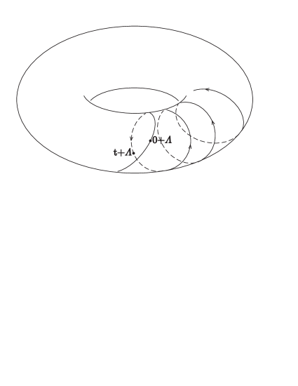
Refer to caption
Figure 2. A fragment of the orbit of ΛΛ\Lambda as seen in the torus parametrization.

Our study of almost periodic functions on ΛΛ\Lambda becomes the study of functions on 𝕋𝕋\mathbb{T} and their restrictions to the ‘spiral’ orbit d+Λsuperscript𝑑Λ\mathbb{R}^{d}+\Lambda in 𝕋𝕋\mathbb{T} given by the embedding (10), i.e. restriction to (d,0)Lsubscriptsuperscript𝑑0𝐿(\mathbb{R}^{d},0)_{L}.

3.4. Fourier coefficients

Let us continue with the situation in §3.3. For all x𝕋𝑥𝕋x\in\mathbb{T},

F~(x)~𝐹𝑥\displaystyle\widetilde{F}(x) =kLake2πik~xabsentsubscript𝑘superscript𝐿subscript𝑎𝑘superscript𝑒2𝜋𝑖inner-product~𝑘𝑥\displaystyle=\sum_{k\in L^{\circ}}a_{k}\,e^{2\pi i\langle\widetilde{k}\mid x\rangle} (19)
whereakwheresubscript𝑎𝑘\displaystyle\text{where}\qquad a_{k} =𝕋e2πik~xF~(x)𝑑θ𝕋(x).absentsubscript𝕋superscript𝑒2𝜋𝑖inner-product~𝑘𝑥~𝐹𝑥differential-dsubscript𝜃𝕋𝑥\displaystyle=\int_{\mathbb{T}}e^{-2\pi i\langle\widetilde{k}\mid x\rangle}\widetilde{F}(x)\,d\theta_{\mathbb{T}}(x)\,. (20)

Unfortunately, we don’t have total control over F~~𝐹\widetilde{F}. We know it only on (d,0)Lsubscriptsuperscript𝑑0𝐿(\mathbb{R}^{d},0)_{L}. To compute aksubscript𝑎𝑘a_{k} out of f𝑓f alone, we use the Birkhoff ergodic theorem333It is hard to find convenient references for the Birkhoff ergodic theorem in the form we need it. Most references prove it over \mathbb{Z} or \mathbb{R}. In [12] there is a proof over dsuperscript𝑑\mathbb{Z}^{d} which is easy to adapt to dsuperscript𝑑\mathbb{R}^{d}. : for all continuous functions G~~𝐺\widetilde{G} on 𝕋𝕋\mathbb{T},

𝕋G~(x)𝑑θ𝕋(x)=limR1volBRBRG~((t,0)L)𝑑t.subscript𝕋~𝐺𝑥differential-dsubscript𝜃𝕋𝑥subscript𝑅1volsubscript𝐵𝑅subscriptsubscript𝐵𝑅~𝐺subscript𝑡0𝐿differential-d𝑡\int_{\mathbb{T}}\widetilde{G}(x)\,d\theta_{\mathbb{T}}(x)=\lim_{R\rightarrow\infty}\frac{1}{\text{vol}\,B_{R}}\int_{B_{R}}\widetilde{G}((t,0)_{L})\,dt\,. (21)

Thus

aksubscript𝑎𝑘\displaystyle a_{k} =limR1volBRBRe2πik~(t,0)F~((t,0)L)𝑑tabsentsubscript𝑅1volsubscript𝐵𝑅subscriptsubscript𝐵𝑅superscript𝑒2𝜋𝑖inner-product~𝑘𝑡0~𝐹subscript𝑡0𝐿differential-d𝑡\displaystyle=\lim_{R\rightarrow\infty}\frac{1}{\text{vol}\,B_{R}}\int_{B_{R}}e^{-2\pi i\langle\widetilde{k}\mid(t,0)\rangle}\widetilde{F}((t,0)_{L})\,dt
=limR1volBRBRe2πiktf(t)𝑑t.absentsubscript𝑅1volsubscript𝐵𝑅subscriptsubscript𝐵𝑅superscript𝑒2𝜋𝑖inner-product𝑘𝑡𝑓𝑡differential-d𝑡\displaystyle=\lim_{R\rightarrow\infty}\frac{1}{\text{vol}\,B_{R}}\int_{B_{R}}e^{-2\pi i\langle k\mid t\rangle}f(t)\,dt\,. (22)

Here we use F((t,0)L)=f(t)𝐹subscript𝑡0𝐿𝑓𝑡F((t,0)_{L})=f(t) and k~=(k,k)~𝑘𝑘superscript𝑘\widetilde{k}=(k,k^{\prime}), so

k~(t,0)=k,t+k,0=k,t.inner-product~𝑘𝑡0𝑘𝑡superscript𝑘0𝑘𝑡\displaystyle\langle\widetilde{k}\mid(t,0)\rangle=\langle k,t\rangle+\langle k^{\prime},0\rangle=\langle k,t\rangle\,.

The averaging sequence {BR}subscript𝐵𝑅\{B_{R}\} that we have employed here can be replaced by any unbounded ascending sequence {An}subscript𝐴𝑛\{A_{n}\}, where Andsubscript𝐴𝑛superscript𝑑A_{n}\subset\mathbb{R}^{d} is compact, An=dsubscript𝐴𝑛superscript𝑑\bigcup A_{n}=\mathbb{R}^{d}, and the boundary of Ansubscript𝐴𝑛A_{n} has measure 0 for all n𝑛n. In actual practice one should adapt the averaging sequence to the problem at hand.

4. Discretization

4.1. Main components

Our objective is to devise a discrete method by which to estimate the coefficients aksubscript𝑎𝑘a_{k} of (22) of a local function f𝑓f with respect to a model set Λ=Λ(Ω)ΛΛΩ\Lambda=\Lambda(\Omega). This means replacing the integral by a finite sum of values of the integrand. The problem is to do this in such a way that it respects the cut and project scheme in which the model set lives, can be guaranteed to converge in the limit to the required integral, and can be carried out efficiently from a computational point of view.

There are three components to this:

  • (i)

    deciding on a suitable domain of integration (what should we use for BRsubscript𝐵𝑅B_{R}?);

  • (ii)

    creating the points of evaluation of the integrand, including how many there should be;

  • (iii)

    deciding to which set of Fourier coefficients (which values of k𝑘k) we should restrict our attention.

A key feature of discrete methods involving periodic functions is the use of finite groups arising from refinements of the period lattice and quotients of its dual lattice, e.g. [20]. We need to translate this concept into the context of cut and project schemes. The set of points on which the integrand is evaluated is created out of the same cut and project process that creates the original model set. The ingredients are a choice of a suitable lattice LN~L~~𝐿~subscript𝐿𝑁\widetilde{L_{N}}\supset\widetilde{L}, which then gives rise to the finite group LN~/L~~subscript𝐿𝑁~𝐿\widetilde{L_{N}}/\widetilde{L}. The data points in dsuperscript𝑑\mathbb{R}^{d} at which computations of our functions will be made come by projection into physical space of a suitable set of coset representatives of LN~~subscript𝐿𝑁\widetilde{L_{N}} modulo L~~𝐿\widetilde{L}. The corresponding frequencies (wave vectors) k𝑘k are chosen from the dual lattice Lsuperscript𝐿L^{\circ}. The choice of values of k𝑘k at which we should evaluate the Fourier coefficients aksubscript𝑎𝑘a_{k} come by selecting suitable representatives of L~superscript~𝐿\widetilde{L}^{\circ} modulo LN~superscript~subscript𝐿𝑁\widetilde{L_{N}}^{\circ}. The key point is the duality

,:L~/LN~×L~N/L~1N/.:superscript~𝐿~superscriptsubscript𝐿𝑁subscript~𝐿𝑁~𝐿1𝑁\displaystyle\langle\cdot\,,\cdot\rangle:\widetilde{L}^{\circ}/\widetilde{L_{N}^{\circ}}\times\widetilde{L}_{N}/\widetilde{L}\longrightarrow\frac{1}{N}\mathbb{Z}/\mathbb{Z}\,.

4.2. Outline of the discretization process

In this section we give more precise details as to how the goals of §4.1 can be achieved. The process necessarily involves a number of decisions, which can only be made in the context of the situation at hand. In §5 and §6 we shall see how this looks in particular examples.

It should be noted that although getting the computational details set up is somewhat involved, these details depend only on the cut and project scheme and the degree of accuracy required from the computation. Once this is established the data points and choices of frequencies are already determined, and they suffice for the Fourier analysis of all functions that arise out of the same almost periodic family, and are algorithmically easy to compute.

We begin with the cut and project scheme (3.1) with torus 𝕋𝕋\mathbb{T} and note the natural extension of the mapping ()superscript(\cdot)^{\prime} to the rational span of the module L𝐿L:

L𝐿\displaystyle\mathbb{Q}L\ 1111\displaystyle\overset{1-1}{\longleftarrow}\quad L~~𝐿\displaystyle\mathbb{Q}\widetilde{L} Lsuperscript𝐿\displaystyle\longrightarrow\quad\mathbb{Q}L^{\prime} (23)
x𝑥\displaystyle x\ absentdivides\displaystyle\leftarrow\!\shortmid x~~𝑥\displaystyle\widetilde{x} =(x,x)absent𝑥superscript𝑥\displaystyle=(x,x^{\prime}) xmaps-tosuperscript𝑥\displaystyle\mapsto\quad\quad x^{\prime}

We assume that 2dd×dsimilar-to-or-equalssuperscript2𝑑superscript𝑑superscript𝑑\mathbb{R}^{2d}\simeq\mathbb{R}^{d}\times\mathbb{R}^{d} is supplied with the standard dot product (denoted |\langle\cdot|\cdot\rangle), and then define the dual lattice:

L~={Yd×d:Yx~for allx~L~}.superscript~𝐿conditional-set𝑌superscript𝑑superscript𝑑inner-product𝑌~𝑥for all~𝑥~𝐿\displaystyle\widetilde{L}^{\circ}=\{Y\in\mathbb{R}^{d}\times\mathbb{R}^{d}\ :\ \langle Y\mid\widetilde{x}\rangle\in\mathbb{Z}\ \;\text{for all}\ \widetilde{x}\in\widetilde{L}\}.

Then L~superscript~𝐿\widetilde{L}^{\circ} is a \mathbb{Z}-module of the same rank as L~~𝐿\widetilde{L}, namely 2d2𝑑2d. There is a cut and project scheme dual to (3.1) of which L~superscript~𝐿\widetilde{L}^{\circ} is the lattice [17]:

dsuperscript𝑑\displaystyle\mathbb{R}^{d}\ ||\displaystyle\overset{||}{\longleftarrow}\quad dsuperscript𝑑\displaystyle\mathbb{R}^{d} ×dabsentsuperscript𝑑\displaystyle\times\mathbb{R}^{d} dperpendicular-tosuperscript𝑑\displaystyle\quad\overset{\perp}{\longrightarrow}\qquad\mathbb{R}^{d}
\displaystyle\cup (24)
Lsuperscript𝐿\displaystyle L^{\circ} 1111\displaystyle\overset{1-1}{\longleftarrow} L~superscript~𝐿\displaystyle\widetilde{L}^{\circ} dense image(L).dense imagesuperscriptsuperscript𝐿\displaystyle\overset{\text{dense image}}{\longrightarrow}\quad(L^{\circ})^{\prime}\,.

We shall use the same type of notation as in (23) for this scheme too. It arises by taking the Pontryagin duals of all the groups in (23), whereupon L~superscript~𝐿\widetilde{L}^{\circ} appears as the dual of the torus 𝕋𝕋\mathbb{T}. For more on dual cut and project schemes see [17].

Dualizing can be considerably simplified if the inner product on d×dsuperscript𝑑superscript𝑑\mathbb{R}^{d}\times\mathbb{R}^{d} is rational valued on the lattice L~~𝐿\widetilde{L}. This quite often happens in actual practice. For instance, it happens in the Fibonacci example below, where the inner product arises from the trace form on [5]delimited-[]5\mathbb{Q}[\sqrt{5}]. When this happens one can identify L~superscript~𝐿\widetilde{L}^{\circ} as a subset of L~~𝐿\mathbb{Q}\widetilde{L} and thereby avoid having to find the new ()superscript(\cdot)^{\prime} mapping. However, in the general situation such simplifications need not exist, and we do not assume them here.

In reading what follows it is good to keep in mind the equation

e2πik~|s~=e2πik|se2πik|ssuperscript𝑒2𝜋𝑖inner-product~𝑘~𝑠superscript𝑒2𝜋𝑖inner-product𝑘𝑠superscript𝑒2𝜋𝑖inner-productsuperscript𝑘superscript𝑠e^{2\pi i\langle\tilde{k}|\tilde{s}\rangle}=e^{2\pi i\langle k|s\rangle}e^{2\pi i\langle k^{\prime}|s^{\prime}\rangle} (25)

which lies at the bottom of the approximation. The discrete Fourier analysis is accomplished by a dual pair of finite groups from which the k~~𝑘\tilde{k} and the s~~𝑠\tilde{s} will come. The actual values of k~~𝑘\tilde{k} and s~~𝑠\tilde{s} are important only modulo the lattices LN~superscript~subscript𝐿𝑁\widetilde{L_{N}}^{\circ} and L~~𝐿\widetilde{L} respectively, and this freedom lies at the heart of the process.

The values of s𝑠s should be in the range A𝐴A of our integration, and ideally we would have the corresponding s=0superscript𝑠0s^{\prime}=0 since the s~~𝑠\tilde{s} are supposed to be representing points of the physical space dsuperscript𝑑\mathbb{R}^{d}. However, the latter is not possible, so we attempt to choose the sA𝑠𝐴s\in A along with ssuperscript𝑠s^{\prime} as small as possible. The approximation then works by throwing away the term which involves k,ssuperscript𝑘superscript𝑠k^{\prime},s^{\prime} in (25). The set of values of k~~𝑘\tilde{k} is constrained primarily by the requirement that the values of |k|𝑘|k| should be small, see the discussion after Step 5 below.

4.3. The six steps

Step 1: Choose a finite subgroup of 𝕋𝕋\mathbb{T} of order N𝑁N. This appears in the form LN~/L~~subscript𝐿𝑁~𝐿\widetilde{L_{N}}/\widetilde{L} where LN~L~~𝐿~subscript𝐿𝑁\widetilde{L_{N}}\supset\widetilde{L} is a lattice refining L~~𝐿\widetilde{L}. The number N𝑁N will determine the number of points of evaluation in approximating the integrals by sums. We have L~NL~subscript~𝐿𝑁~𝐿\widetilde{L}_{N}\subset\mathbb{Q}\widetilde{L} and it has a \mathbb{Z}-dual L~NL~superscriptsubscript~𝐿𝑁superscript~𝐿\widetilde{L}_{N}^{\circ}\subset\widetilde{L}^{\circ} which is of index N𝑁N in L~superscript~𝐿\widetilde{L}^{\circ}.

This affords the natural pairing

L~/L~N×L~N/L~1N/superscript~𝐿superscriptsubscript~𝐿𝑁subscript~𝐿𝑁~𝐿1𝑁\widetilde{L}^{\circ}/\widetilde{L}_{N}^{\circ}\times\widetilde{L}_{N}/\widetilde{L}\quad\longrightarrow\quad\frac{1}{N}\mathbb{Z}/\mathbb{Z} (26)

induced by \langle\cdot\mid\cdot\rangle (and still denoted by \langle\cdot\mid\cdot\rangle). Using the ()superscript(\cdot)^{\prime} mappings, we obtain, in the obvious notation, the \mathbb{Z}-modules LNL𝐿subscript𝐿𝑁L_{N}\supset L , LNLsuperscriptsubscript𝐿𝑁superscript𝐿L_{N}^{\circ}\subset L^{\circ}, L~N/L~LN/Lsimilar-to-or-equalssubscript~𝐿𝑁~𝐿subscript𝐿𝑁𝐿\widetilde{L}_{N}/\widetilde{L}\simeq L_{N}/L, L~/L~NL~/L~Nsimilar-to-or-equalssuperscript~𝐿superscriptsubscript~𝐿𝑁~𝐿subscript~𝐿𝑁\widetilde{L}^{\circ}/\widetilde{L}_{N}^{\circ}\simeq\widetilde{L}/\widetilde{L}_{N}, and an induced pairing

:L/LN×LN/L1N/.\displaystyle\langle\cdot\mid\cdot\rangle\ :\ L^{\circ}/L_{N}^{\circ}\times L_{N}/L\quad\longrightarrow\quad\frac{1}{N}\mathbb{Z}/\mathbb{Z}\,.

Replacing L~~𝐿\widetilde{L} by L~Nsubscript~𝐿𝑁\widetilde{L}_{N}, we have the refined cut and project scheme

dsuperscript𝑑\displaystyle\mathbb{R}^{d} \displaystyle\quad\longleftarrow\quad dsuperscript𝑑\displaystyle\mathbb{R}^{d} ×dabsentsuperscript𝑑\displaystyle\times\mathbb{R}^{d} \displaystyle\quad\longrightarrow\quad dsuperscript𝑑\displaystyle\mathbb{R}^{d} (27)
\displaystyle\cup
LNsubscript𝐿𝑁\displaystyle L_{N} 1111\displaystyle\quad\overset{1-1}{\longleftrightarrow}\quad L~Nsubscript~𝐿𝑁\displaystyle\widetilde{L}_{N} \displaystyle\quad\longleftrightarrow\quad LNsuperscriptsubscript𝐿𝑁\displaystyle L_{N}^{\prime}

and similarly its dual.

Step 2: Choose a fundamental domain C𝐶C for L~~𝐿\widetilde{L}. A canonical choice would be the Voronoi cell of L~~𝐿\widetilde{L} at 0, but any other choice is allowable. In the examples below we use the parallelogram defined by a pair of basis vectors of L~~𝐿\widetilde{L}. Cover (d,0)2dsuperscript𝑑0superscript2𝑑(\mathbb{R}^{d},0)\subset\mathbb{R}^{2d} with a set of translates t~+C~𝑡𝐶\tilde{t}+C of C𝐶C by elements of L~~𝐿\widetilde{L}. The projection of these cells into the physical space dsuperscript𝑑\mathbb{R}^{d} covers it, though in general the projected t~+C~𝑡𝐶\tilde{t}+C have many overlaps.

Step 3: Form S~:=LN~Cassign~𝑆~subscript𝐿𝑁𝐶\widetilde{S}:=\widetilde{L_{N}}\cap C. This provides a complete set of representatives in LN~~subscript𝐿𝑁\widetilde{L_{N}} for the group L~N/L~subscript~𝐿𝑁~𝐿\widetilde{L}_{N}/\widetilde{L}.

Step 4: Choose a region A𝐴A which will be the delimiting the range over which the Fourier coefficients of f𝑓f will be estimated in the form

ak=ak~1volAAe2πiktf(t)𝑑t.subscript𝑎𝑘subscript𝑎~𝑘similar-to-or-equals1vol𝐴subscript𝐴superscript𝑒2𝜋𝑖inner-product𝑘𝑡𝑓𝑡differential-d𝑡\displaystyle a_{k}=a_{\widetilde{k}}\simeq\frac{1}{\text{vol}\,A}\int_{A}e^{-2\pi i\langle k\mid t\rangle}f(t)\,dt.

These integrals have to be computed for values of k𝑘k that come from L/LNsuperscript𝐿subscriptsuperscript𝐿𝑁L^{\circ}/L^{\circ}_{N}.

Take as A𝐴A the image of a finite set of the translates of C𝐶C appearing in Step 2, i.e.

A=(t~T~t~+C)||\displaystyle A=(\bigcup_{\tilde{t}\in\widetilde{T}}\tilde{t}+C)^{||}

for some finite subset of T~~𝑇\widetilde{T} elements of L~~𝐿\widetilde{L}. The choice of A𝐴A is again determined by the problem at hand.

We need next to determine a set of data points in dsuperscript𝑑\mathbb{R}^{d} which will serve to replace the integrals of Step 4 by finite sums. This is the purpose of the next step.

As we pointed out above, we are free to translate the elements of S~~𝑆\widetilde{S} by L~~𝐿\widetilde{L} as we please, and we wish to do this so that the projected images are in our region of integration A=t~T~(t~+C)||A=\bigcup_{\tilde{t}\in\widetilde{T}}(\tilde{t}+C)^{||}. We also keep in mind that we wish to do this so as to minimize the size of the corresponding ssuperscript𝑠s^{\prime}.

Step 5: For each s~=(s,s)S~~𝑠𝑠superscript𝑠~𝑆\tilde{s}=(s,s^{\prime})\in\widetilde{S} find a t(s)~T~~𝑡𝑠~𝑇\widetilde{t(s)}\in\widetilde{T} for which |s+t(s)|superscript𝑠𝑡superscript𝑠|s^{\prime}+t(s)^{\prime}| is minimal. Then the set of data points is

D:={s+t(s):s~S~}.assign𝐷conditional-set𝑠𝑡𝑠~𝑠~𝑆\displaystyle D:=\{s+t(s)\,:\,\widetilde{s}\in\widetilde{S}\}.

At this point, for each kL𝑘superscript𝐿k\in L^{\circ} we have

ak:=1volAuDe2πik|uf(u)assignsubscript𝑎𝑘1vol𝐴subscript𝑢𝐷superscript𝑒2𝜋𝑖inner-product𝑘𝑢𝑓𝑢\displaystyle a_{k}:=\frac{1}{{\rm vol}\,A}\sum_{u\in D}e^{-2\pi i\langle k|u\rangle}f(u)

and the resulting approximation of f𝑓f is

f(x)kKake2πik|x.similar-to-or-equals𝑓𝑥subscript𝑘𝐾subscript𝑎𝑘superscript𝑒2𝜋𝑖inner-product𝑘𝑥\displaystyle f(x)\simeq\sum_{k\in K}a_{k}e^{2\pi i\langle k|x\rangle}.

The set K𝐾K is to run over a complete set of representatives of L/LNsuperscript𝐿superscriptsubscript𝐿𝑁L^{\circ}/L_{N}^{\circ}. The choice seems free, but one may assume that in most cases the lower frequencies (smaller |k|𝑘|k|) are most essential in approximating f𝑓f by using only finitely many of its frequencies. For this reason we have:

Step 6: Choose k𝑘k for each class of L/LNsuperscript𝐿superscriptsubscript𝐿𝑁L^{\circ}/L_{N}^{\circ} with |k|𝑘|k| taken as small as possible.

This concludes the broad description of the algorithm.

5. A Fibonacci example

To make all this more concrete we work through the details of a one dimensional example, the well-known Fibonacci sequence, where the cut and project scheme lives in two dimensions and the geometry of the data set D𝐷D and the set of translates T~~𝑇\tilde{T} via a refinement lattice and new windows are easily visualized. This involves first setting up the cut and project scheme in detail, §5.1 and §5.2, and then describing a Fibonacci point set arising from the standard Fibonacci substitution in terms of it, §5.3. We then follow Steps 1 through 6 of §4.3, which provide the data points and corresponding frequencies that will work for the analysis of any local function that we may choose. In §6 we apply this information to two simple examples of local functions to see how well the methods actually work.

One of the great virtues of the cut and project method is that it is primarily an algebraic tool and does not require great geometric insight to use it. Given that for aperiodic structures in dimension greater than 111 we almost always in the situation of lattices of rank greater than 333, and hence forced into spaces in dimensions greater than 333, this type of algebraic formalism is of enormous value. However, in the Fibonacci example, in which everything can be done in 222-dimensions, it is useful to see the underlying geometry explicitly. Thus we have gone to some effort to show the geometric meaning of the central feature of the method, that is, the creation of the data points, and to show what the approximations look like and how good they are in comparison with exact computation. In actual practice all this is unnecessary. The only part of the algorithm that requires any serious insight into the geometry (and it is actually trivial in the Fibonacci example) is the selection of the fundamental domain and the translates of it that are to be used. It is their projection that makes the domain in physical space in which the data will lie.

5.1. The Fibonacci cut and project scheme

Let τ:=12(1+5)assign𝜏1215\tau:=\tfrac{1}{2}(1+\sqrt{5}) and let Z[τ]=+τ𝑍delimited-[]𝜏𝜏Z[\tau]=\mathbb{Z}+\mathbb{Z}\tau. Then Z[τ]𝑍delimited-[]𝜏Z[\tau] is the ring of integers of the field [τ]=[5]delimited-[]𝜏delimited-[]5\mathbb{Q}[\tau]=\mathbb{Q}[\sqrt{5}] and τ2=τ+1superscript𝜏2𝜏1\tau^{2}=\tau+1. Let ()superscript(\cdot)^{\prime} on Z[τ]𝑍delimited-[]𝜏Z[\tau] and [τ]delimited-[]𝜏\mathbb{Q}[\tau] be the conjugation that interchanges 55\sqrt{5} and 55-\sqrt{5}.

We define

[τ]~:={(x,x):x[τ]}×.assign~delimited-[]𝜏conditional-set𝑥superscript𝑥𝑥delimited-[]𝜏\displaystyle\widetilde{\mathbb{Z}[\tau]}:=\{(x,x^{\prime})\ :\ x\in\mathbb{Z}[\tau]\}\subset\mathbb{R}\times\mathbb{R}\,.

[τ]~~delimited-[]𝜏\widetilde{\mathbb{Z}[\tau]} is a lattice in ×\mathbb{R}\times\mathbb{R} and its natural projections

×\displaystyle\mathbb{R}\leftarrow\!\shortmid\mathbb{R}\times\mathbb{R}\mapsto\mathbb{R}

into \mathbb{R} provide the set-up for the Fibonacci cut-and-project scheme:

\displaystyle\mathbb{R} \displaystyle\longleftarrow\quad \displaystyle\mathbb{R} ×absent\displaystyle\times\mathbb{R} \displaystyle\longrightarrow\quad \displaystyle\mathbb{R} (28)
\displaystyle\cup \displaystyle\cup \displaystyle\cup
[τ]delimited-[]𝜏\displaystyle\mathbb{Z}[\tau] \displaystyle\quad\longleftarrow\quad [τ]~~delimited-[]𝜏\displaystyle\widetilde{\mathbb{Z}[\tau]} \displaystyle\quad\longrightarrow\quad [τ]delimited-[]𝜏\displaystyle\mathbb{Z}[\tau]
x𝑥\displaystyle x absentdivides\displaystyle\quad\leftarrow\!\shortmid\quad x~~𝑥\displaystyle\widetilde{x} =(x,x)absent𝑥superscript𝑥\displaystyle=(x,x^{\prime}) maps-to\displaystyle\quad\mapsto\quad x.superscript𝑥\displaystyle x^{\prime}\,.

A natural basis of [τ]~~delimited-[]𝜏\widetilde{\mathbb{Z}[\tau]} is {(1,1)\{(1,1), (τ,τ)}(\tau,\tau^{\prime})\} and the standard inner product on [τ]~~delimited-[]𝜏\widetilde{\mathbb{Z}[\tau]} is defined by

(x~y~)=(2xy)=δxy+(δxy),conditional~𝑥~𝑦subscript2𝑥𝑦𝛿𝑥𝑦superscript𝛿𝑥𝑦(\widetilde{x}\mid\widetilde{y})=(2x\cdot y)_{\mathbb{Z}}=\delta xy+(\delta xy)^{\prime}\,, (29)

Here the notation ()subscript(\ \cdot\ )_{\mathbb{Z}} indicates taking the rational component a𝑎a of 2xy[τ]=:a+bτ2x\cdot y\in\mathbb{Z}[\tau]=:a+b\tau, and

δ𝛿\displaystyle\delta =(τ5)1=(τ(ττ))1=1τ2+1,absentsuperscript𝜏51superscript𝜏𝜏superscript𝜏11superscript𝜏21\displaystyle=(\tau\sqrt{5})^{-1}=(\tau(\tau-\tau^{\prime}))^{-1}=\tfrac{1}{\tau^{2}+1}\,,
δsuperscript𝛿\displaystyle\delta^{\prime} =(τ5)1=(τ(ττ))1=1τ2+1,absentsuperscriptsuperscript𝜏51superscriptsuperscript𝜏superscript𝜏𝜏11superscript𝜏21\displaystyle=(-\tau^{\prime}\sqrt{5})^{-1}=(\tau^{\prime}(\tau^{\prime}-\tau))^{-1}=\tfrac{1}{\tau^{\prime 2}+1}\,, (30)

In particular,

(1~1~)=(2(11))=2,(τ~τ~)=(2τ2)=2,(1~τ~)=(2τ)=0.formulae-sequenceconditional~1~1subscript2112conditional~𝜏~𝜏subscript2superscript𝜏22conditional~1~𝜏subscript2𝜏0\displaystyle(\widetilde{1}\mid\widetilde{1})=(2(1\cdot 1))_{\mathbb{Z}}=2\,,\quad(\widetilde{\tau}\mid\widetilde{\tau})=(2\tau^{2})_{\mathbb{Z}}=2\,,\quad(\widetilde{1}\mid\widetilde{\tau})=(2\tau)_{\mathbb{Z}}=0\,.

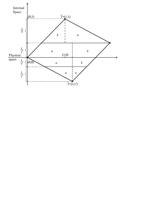
The geometry of the fundamental cell for the lattice [τ]~~delimited-[]𝜏\widetilde{\mathbb{Z}[\tau]} is illustrated in Fig. 3. More details of the material here can be found in [10].

5.2. The dual lattice

The inner product ()(\cdot\mid\cdot) allows us to identify [τ]~superscript~delimited-[]𝜏\widetilde{\mathbb{Z}[\tau]}^{\circ} inside the rational span of [τ]~~delimited-[]𝜏\widetilde{\mathbb{Z}[\tau]} and to express \langle\cdot\mid\cdot\rangle in terms of ()(\cdot\mid\cdot). The basis dual to {(1,1),(τ,τ)}11𝜏superscript𝜏\{(1,1),(\tau,\tau^{\prime})\} is given by

ω~1=121~=(12,12),ω~2=12τ~=(τ2,τ2),formulae-sequencesubscript~𝜔112~11212subscript~𝜔212~𝜏𝜏2superscript𝜏2\widetilde{\omega}_{1}=\tfrac{1}{2}\widetilde{1}=(\tfrac{1}{2},\tfrac{1}{2})\,,\qquad\widetilde{\omega}_{2}=\tfrac{1}{2}\widetilde{\tau}=(\tfrac{\tau}{2},\tfrac{\tau^{\prime}}{2})\,, (31)

and the dual lattice is

([τ]~)=ω~1+ω~2=12[τ]~.superscript~delimited-[]𝜏subscript~𝜔1subscript~𝜔212~delimited-[]𝜏({\widetilde{\mathbb{Z}[\tau]})^{\circ}}=\mathbb{Z}\widetilde{\omega}_{1}+\mathbb{Z}\widetilde{\omega}_{2}=\tfrac{1}{2}\widetilde{\mathbb{Z}[\tau]}\,. (32)

The elements of ([τ]~)superscript~delimited-[]𝜏({\widetilde{\mathbb{Z}[\tau]})^{\circ}} are always of the form k~=(k,k)~𝑘𝑘superscript𝑘\widetilde{k}=(k,k^{\prime}) and we can write

[τ]:={k:k~=(k,k)([τ]~)}assignsuperscriptdelimited-[]𝜏conditional-set𝑘~𝑘𝑘superscript𝑘superscript~delimited-[]𝜏\mathbb{Z}[\tau]^{\circ}:=\{k\ :\ \widetilde{k}=(k,k^{\prime})\in({\widetilde{\mathbb{Z}[\tau]})^{\circ}}\} (33)

Then

([τ]~)=[τ]~={k~:k=(k,k)[τ]},superscript~delimited-[]𝜏~superscriptdelimited-[]𝜏conditional-set~𝑘𝑘𝑘superscript𝑘superscriptdelimited-[]𝜏(\widetilde{\mathbb{Z}[\tau]})^{\circ}=\widetilde{\mathbb{Z}[\tau]^{\circ}}=\{\widetilde{k}\ :\ k=(k,k^{\prime})\in\mathbb{Z}[\tau]^{\circ}\}\,,

and k~x~inner-product~𝑘~𝑥\langle\widetilde{k}\mid\widetilde{x}\rangle becomes (k~x~)conditional~𝑘~𝑥(\widetilde{k}\mid\widetilde{x}), which is more useful notation for the sequel.

The 2-torus 𝕋𝕋\mathbb{T} of the cut-and-project scheme (28) is then

𝕋=(×)/[τ]~.𝕋~delimited-[]𝜏\displaystyle\mathbb{T}=(\mathbb{R}\times\mathbb{R})/\widetilde{\mathbb{Z}[\tau]}\,.

Fourier series on 𝕋𝕋\mathbb{T} are expressed in terms of the characters χk~subscript𝜒~𝑘\chi_{\widetilde{k}}, namely

χk~(x~)=e2πi(k~x~),wherek~=(k,k)ω~1+ω~2.formulae-sequencesubscript𝜒~𝑘~𝑥superscript𝑒2𝜋𝑖conditional~𝑘~𝑥where~𝑘𝑘superscript𝑘subscript~𝜔1subscript~𝜔2\chi_{\widetilde{k}}({\widetilde{x}})=e^{2\pi i(\widetilde{k}\mid\widetilde{x})}\,,\quad\text{where}\quad\widetilde{k}=(k,k^{\prime})\in\mathbb{Z}\widetilde{\omega}_{1}+\mathbb{Z}\widetilde{\omega}_{2}\,. (34)

Here x~~𝑥\widetilde{x} can be arbitrary in ×\mathbb{R}\times\mathbb{R}, but we shall need to compute only with x~ω~1+ω~2~𝑥subscript~𝜔1subscript~𝜔2\widetilde{x}\in\mathbb{Q}\widetilde{\omega}_{1}+\mathbb{Q}\widetilde{\omega}_{2} for which ~~absent\widetilde{\ } is well-defined (28). For these elements (k~x~)=(2kx)conditional~𝑘~𝑥subscript2𝑘𝑥(\widetilde{k}\mid\widetilde{x})=(2k\cdot x)_{\mathbb{Q}}.

The product ()(\cdot\mid\cdot) extends to ×\mathbb{R}\times\mathbb{R}, but care has to be taken. For a typical element a1~+bτ~𝑎~1𝑏~𝜏a\widetilde{1}+b\widetilde{\tau}, a,b𝑎𝑏a,b\in\mathbb{R} of our superspace ×\mathbb{R}\times\mathbb{R} the inner product is calculated as

((a1~+bτ~)(c1~+dτ~))=2ac+2bd,conditional𝑎~1𝑏~𝜏𝑐~1𝑑~𝜏2𝑎𝑐2𝑏𝑑\displaystyle((a\widetilde{1}+b\widetilde{\tau})\mid(c\widetilde{1}+d\widetilde{\tau}))=2ac+2bd\,,

where

a1~+bτ~=a(1,1)+b(τ,τ)=(a+bτ,a+bτ)×.𝑎~1𝑏~𝜏𝑎11𝑏𝜏superscript𝜏𝑎𝑏𝜏𝑎𝑏superscript𝜏\displaystyle a\widetilde{1}+b\widetilde{\tau}=a(1,1)+b(\tau,\tau^{\prime})=(a+b\tau,a+b\tau^{\prime})\in\mathbb{R}\times\mathbb{R}\,.

Consider

k~=aω~1+bω~2=a21~+b2τ~=(a+bτ2,a+bτ2)=(k,k)[τ]~,~𝑘𝑎subscript~𝜔1𝑏subscript~𝜔2𝑎2~1𝑏2~𝜏𝑎𝑏𝜏2𝑎𝑏superscript𝜏2𝑘superscript𝑘superscript~delimited-[]𝜏\displaystyle\widetilde{k}=a\widetilde{\omega}_{1}+b\widetilde{\omega}_{2}=\tfrac{a}{2}\widetilde{1}+\tfrac{b}{2}\widetilde{\tau}=\left(\tfrac{a+b\tau}{2},\tfrac{a+b\tau^{\prime}}{2}\right)=(k,k^{\prime})\in\widetilde{\mathbb{Z}[\tau]}^{\circ}\,,

where a,b𝑎𝑏a,b\in\mathbb{Z}. Suppose we want to compute (k~(t,0))conditional~𝑘𝑡0(\widetilde{k}\mid(t,0)), t𝑡t\in\mathbb{R}. From

(1,0)10\displaystyle(1,0) =1τ51~+15τ~absent1𝜏5~115~𝜏\displaystyle=\tfrac{1}{\tau\sqrt{5}}\widetilde{1}+\tfrac{1}{\sqrt{5}}\widetilde{\tau} =δ1~+τδτ~,absent𝛿~1𝜏𝛿~𝜏\displaystyle=\delta\widetilde{1}+\tau\delta\widetilde{\tau}\,,
(0,1)01\displaystyle(0,1) =τ2δ1~τδτ~absentsuperscript𝜏2𝛿~1𝜏𝛿~𝜏\displaystyle=\tau^{2}\delta\widetilde{1}-\tau\delta\widetilde{\tau} =δ1~+τδτ~,absentsuperscript𝛿~1superscript𝜏superscript𝛿~𝜏\displaystyle=\delta^{\prime}\widetilde{1}+\tau^{\prime}\delta^{\prime}\widetilde{\tau}\,,

where δ,δ𝛿superscript𝛿\delta,\ \delta^{\prime} are from (5.1), we have

(k~(1,0))=2δk,conditional~𝑘102𝛿𝑘\displaystyle(\widetilde{k}\mid(1,0))=2\delta k\,,

and so,

(k~(t,0))=2δkt,for allt.formulae-sequenceconditional~𝑘𝑡02𝛿𝑘𝑡for all𝑡\displaystyle(\widetilde{k}\mid(t,0))=2\delta kt\,,\qquad\text{for all}\quad t\in\mathbb{R}.

We are interested in model sets ΛΛ\Lambda coming from the cut and project scheme (28). In the context of (28), the Fourier-Bohr expansion (18) assumes the simpler form

f(t)=F(t+Λ)=F~((t,0)[τ]~)=k[τ]ake2πi2δkt.𝑓𝑡𝐹𝑡Λ~𝐹subscript𝑡0~delimited-[]𝜏subscript𝑘superscriptdelimited-[]𝜏subscript𝑎𝑘superscript𝑒2𝜋𝑖2𝛿𝑘𝑡f(t)=F(t+\Lambda)=\widetilde{F}((t,0)_{\widetilde{\mathbb{Z}[\tau]}})\\ =\sum_{k\in\mathbb{Z}[\tau]^{\circ}}a_{k}\,e^{2\pi i2\delta kt}\,. (35)

We shall use the aksubscript𝑎𝑘a_{k} computed in the form

ak=limR1R0Re2πi2ktf(t)𝑑t.subscript𝑎𝑘subscript𝑅1𝑅superscriptsubscript0𝑅superscript𝑒2𝜋𝑖2𝑘𝑡𝑓𝑡differential-d𝑡\displaystyle a_{k}=\lim_{R\to\infty}\frac{1}{R}\int_{0}^{R}e^{-2\pi i2kt}\,f(t)dt.

For future use note that

(k~(0,1))conditional~𝑘01\displaystyle(\widetilde{k}\mid(0,1)) =((a+bτ2,a+bτ2)δ1~+τδτ~)=2kδabsentconditional𝑎𝑏𝜏2𝑎𝑏superscript𝜏2superscript𝛿~1superscript𝜏superscript𝛿~𝜏2superscript𝑘superscript𝛿\displaystyle=((\tfrac{a+b\tau}{2},\tfrac{a+b\tau^{\prime}}{2})\mid\delta^{\prime}\widetilde{1}+\tau^{\prime}\delta^{\prime}\widetilde{\tau})=2k^{\prime}\delta^{\prime}
(k~(0,u))conditional~𝑘0𝑢\displaystyle(\widetilde{k}\mid(0,u)) =2ukδ.absent2𝑢superscript𝑘superscript𝛿\displaystyle=2uk^{\prime}\delta^{\prime}\,. (36)

5.3. The Fibonacci model set

The standard 222-letter Fibonacci sequence is the fixed point of the substitution aab𝑎𝑎𝑏a\rightarrow ab, ba𝑏𝑎b\rightarrow a: namely,

abaababa.𝑎𝑏𝑎𝑎𝑏𝑎𝑏𝑎\displaystyle abaababa\dots\ .

With tile lengths τ𝜏\tau for a𝑎a symbols and 111 for b𝑏b symbols, and starting at 00, we get the sequence of tiles that cover the non-negative part of the real line. The left-hand ends of these tiles,

0,τ,τ+1, 2τ+1, 3τ+1, 3τ+2, 4τ+2, 4τ+3, 5τ+3,0𝜏𝜏12𝜏13𝜏13𝜏24𝜏24𝜏35𝜏3\displaystyle 0,\,\tau,\,\tau+1,\,2\tau+1,\,3\tau+1,\,3\tau+2,\,4\tau+2,\,4\tau+3,\,5\tau+3,\,\dots

form an infinite sequence of points on the non-negative real line. This set appears explicitly as the non-negative part of the model set

Λ=Λ([1,1τ))ΛΛ11𝜏\displaystyle\Lambda=\Lambda([-1,\tfrac{1}{\tau}))

arising from the cut and project scheme (28).444Alternatively one can use Λ((1,1τ])Λ11𝜏\Lambda((-1,\frac{1}{\tau}]), which differs from ΛΛ\Lambda in the two points coming from the ends of the interval [1,1τ)11𝜏[-1,\frac{1}{\tau}). This is an example of a pair of sets that map to the same place in 𝕋𝕋\mathbb{T}. This ambiguity shows up in an interesting way later on, see §6.3. ΛΛ\Lambda decomposes as Λa=Λ([1τ2,1τ))subscriptΛ𝑎Λ1superscript𝜏21𝜏\Lambda_{a}=\Lambda([-\frac{1}{\tau^{2}},\frac{1}{\tau})) and Λb=Λ([1,1τ2))subscriptΛ𝑏Λ11superscript𝜏2\Lambda_{b}=\Lambda([-1,-\frac{1}{\tau^{2}})), which give the left-hand end points of the a𝑎a and b𝑏b points respectively.

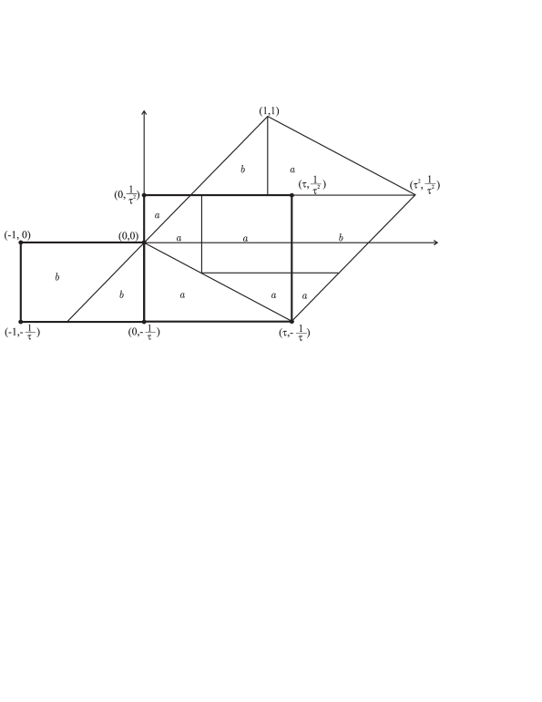
Refer to caption
Figure 3. The fundamental cell C𝐶C of the lattice [τ]~=(1,1)+(τ,τ)~delimited-[]𝜏11𝜏superscript𝜏\widetilde{\mathbb{Z}[\tau]}=\mathbb{Z}(1,1)+\mathbb{Z}(\tau,\tau^{\prime}) is shown in terms of the standard coordinate system for ×\mathbb{R}\times\mathbb{R}. When C𝐶C is imagined as a torus by identifying opposite sides and the physical space is wrapped onto it using these identifications, then the a𝑎a and b𝑏b regions shown here indicate which parts of the physical space are lying in a𝑎a or b𝑏b tiles respectively.

A useful and commonly used way to visualize the distribution of a𝑎a and b𝑏b points is to view them on the torus 𝕋𝕋\mathbb{T} after the embedding (10) of \mathbb{R} in 𝕋𝕋\mathbb{T}. The fundamental cell, see Fig. 3, with opposite edges identified is 𝕋𝕋\mathbb{T}. To see ΛΛ\Lambda itself being formed, we start at (0,0)00(0,0) and trace out (t,0)𝑡0(t,0), t𝑡t\in\mathbb{R}, with the usual rules for exiting and re-entering the fundamental cell. We move continuously. Our moving point has three ‘whiskers’ attached to it.

a(1)𝑎1a(1): a whisker of length 1τ1𝜏\tfrac{1}{\tau} facing vertically upwards;

a(2)𝑎2a(2): a whisker of length 1τ21superscript𝜏2\tfrac{1}{\tau^{2}} facing down;

b(1)𝑏1b(1): a whisker of length 1τ1𝜏\tfrac{1}{\tau} that faces down, but has an initial gap of size 1τ21superscript𝜏2\tfrac{1}{\tau^{2}}.

The rule is this. As our point moves along the line on the fundamental cell, if the a(1)𝑎1a(1) whisker hits (1,1)11(1,1) (i.e. (1,1)11(1,1) is close enough to get cut by this whisker), we get an a𝑎a-point of ΛΛ\Lambda. If the a(2)𝑎2a(2) whisker hits the point (τ,τ)𝜏superscript𝜏(\tau,\tau^{\prime}), we also get an a𝑎a-point of ΛΛ\Lambda. If the b(1)𝑏1b(1) whisker hits the point (τ,τ)𝜏superscript𝜏(\tau,\tau^{\prime}), we get a b𝑏b-point.

Essentially the window, represented by the whiskers, is carried along with the moving point, and exits and re-enters the fundamental cell with the moving point.

The advantage of this point of view is that it allows us to divide the fundamental cell into regions which deliver the a𝑎a- and b𝑏b-points, and thus to see what our function f(t)𝑓𝑡f(t) looks like on the fundamental cell.

In Fig. 3 the vertical dotted lines are the key thing. Our moving point moves to the right and every time it crosses a dotted vertical line, we get a new point of ΛΛ\Lambda, thus starting a new interval. We stay on that interval until the next crossing.

The a𝑎a and b𝑏b regions are indicated in the Fig. 3.

5.4. Discretization

We now go into the details of how to deal with the Fourier analysis using discrete methods. Here we follow the six steps outlined in §4.3.

Write L~~𝐿\widetilde{L} for [τ]~~delimited-[]𝜏\widetilde{\mathbb{Z}[\tau]}, so L~=1~+τ~~𝐿~1~𝜏\widetilde{L}=\mathbb{Z}\widetilde{1}+\mathbb{Z}\widetilde{\tau}. Let C:={u1~+vτ~: 0u,v>1}assign𝐶conditional-set𝑢~1𝑣~𝜏formulae-sequence 0𝑢𝑣1C:=\{u\widetilde{1}+v\widetilde{\tau}\ :\ 0\leq u,v>1\} be a fundamental region for L~~𝐿\widetilde{L}. Its volume is equal to 55\sqrt{5} .

Fix any N+𝑁subscriptN\in\mathbb{Z}_{+}. We want to create a lattice LN~~subscript𝐿𝑁\widetilde{L_{N}} that is a refinement of L~~𝐿\widetilde{L}. In the §4.3 we took LN~L~~𝐿~subscript𝐿𝑁\widetilde{L_{N}}\supset\widetilde{L} with [LN~:L~]=N[\widetilde{L_{N}}:\widetilde{L}]=N. In our present situation we use the most obvious lattices, namely 1NL1𝑁𝐿\frac{1}{N}L. These actually have index N2superscript𝑁2N^{2}, so there are some slight notational differences between this section and §4.3. Since NLN~L~𝑁~subscript𝐿𝑁~𝐿N\widetilde{L_{N}}\subseteq\widetilde{L}, so LN~1~+τ~~subscript𝐿𝑁~1~𝜏\widetilde{L_{N}}\subset\mathbb{Q}\widetilde{1}+\mathbb{Q}\widetilde{\tau}.

Let S~:=LNCassign~𝑆subscript𝐿𝑁𝐶\tilde{S}:=L_{N}\cap C, so S~~𝑆\tilde{S} is a complete set of representatives of LNmodLmodulosubscript𝐿𝑁𝐿L_{N}\mod L.

Together this completes steps 1, 2, 3 of §4.2.

For understanding the approximations better we also introduce a fundamental region CNsubscript𝐶𝑁C_{N} for LNsubscript𝐿𝑁L_{N}, chosen so that

C=s~S~s~+CN.𝐶subscript~𝑠~𝑆~𝑠subscript𝐶𝑁C=\bigcup_{\tilde{s}\in\tilde{S}}\tilde{s}+C_{N}\,. (37)

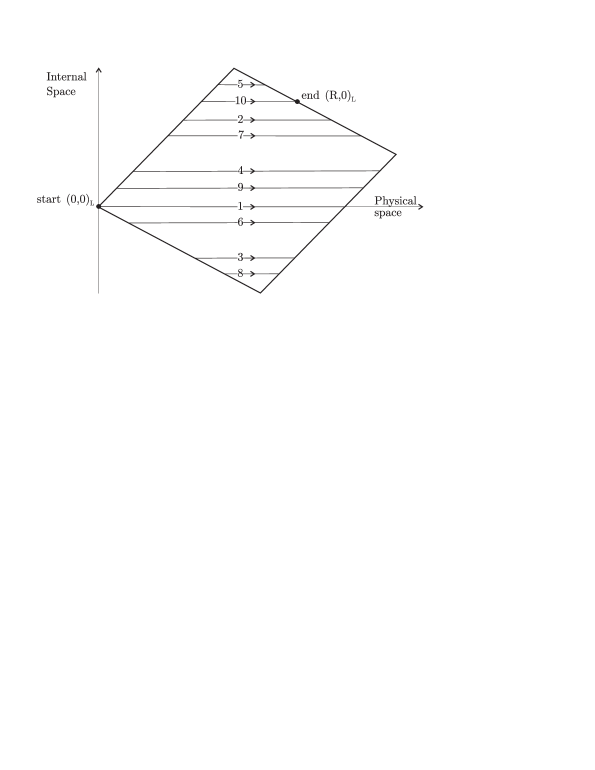
For Step 4 we choose as our delimiting range in \mathbb{R} an interval [0,R]0𝑅[0,R] where R𝑅R is a positive real number taken so that (R,0)𝑅0(R,0) taken modulo L~~𝐿\widetilde{L} is on the boundary of C𝐶C. Following along the path (t,0)𝑡0(t,0), t>0𝑡subscriptabsent0t\in\mathbb{R}_{>0}, and wrapping around C𝐶C as indicated in Fig. 4, this amounts to stopping at some point R𝑅R where the path is just exiting C𝐶C, so that we have an exact number of passes of C𝐶C. Thus the path (t,0)𝑡0(t,0), 0tR0𝑡𝑅0\leq t\leq R involves an explicit set of translates t~i+Csubscript~𝑡𝑖𝐶\tilde{t}_{i}+C, i=1,,M𝑖1𝑀i=1,\dots,M of C𝐶C. Let T~={t~1,,t~M}~𝑇subscript~𝑡1subscript~𝑡𝑀\tilde{T}=\{\tilde{t}_{1},\dots,\tilde{t}_{M}\}.

Let f::𝑓f:\mathbb{R}\rightarrow\mathbb{C} be any continuous local function with respect to the model set Λ=Λ([1,1τ))ΛΛ11𝜏\Lambda=\Lambda([-1,\tfrac{1}{\tau})), and let F~:𝕋:~𝐹𝕋\widetilde{F}:\mathbb{T}\rightarrow\mathbb{C} be its extension to a continuous function on 𝕋=R2/L~𝕋superscript𝑅2~𝐿\mathbb{T}=R^{2}/\widetilde{L}. Generally we are interested in Fourier decomposition of F~~𝐹\widetilde{F} and along with it the corresponding decomposition of f𝑓f. Thus we wish to compute things like

𝕋F~(x)e2πi(k~x)𝑑θ𝕋(x).subscript𝕋~𝐹𝑥superscript𝑒2𝜋𝑖conditional~𝑘𝑥differential-dsubscript𝜃𝕋𝑥\displaystyle\int_{\mathbb{T}}\widetilde{F}(x)\,e^{-2\pi i(\widetilde{k}\mid x)}d\theta_{\mathbb{T}}(x)\,.

Here F~()e2πi(k~)~𝐹superscript𝑒2𝜋𝑖conditional~𝑘\widetilde{F}(\cdot)e^{-2\pi i(\widetilde{k}\mid\cdot)} is just some other continuous function on 𝕋𝕋\mathbb{T} that is local with respect to ΛΛ\Lambda. So it suffices to deal with some general continuous function G~~𝐺\widetilde{G} on 𝕋𝕋\mathbb{T} and its restriction g(t)=G~((t,0))𝑔𝑡~𝐺𝑡0g(t)=\widetilde{G}((t,0)) to the line (,0)modL~modulo0~𝐿(\mathbb{R},0)\mod\widetilde{L}.

Let

εN:=supi=1,,N2supxs~i+CN|G~(x)G~(s~i)|.assignsubscript𝜀𝑁subscriptsupremum𝑖1superscript𝑁2subscriptsupremum𝑥subscript~𝑠𝑖subscript𝐶𝑁~𝐺𝑥~𝐺subscript~𝑠𝑖\displaystyle\varepsilon_{N}:=\sup_{i=1,\dots,N^{2}}\ \sup_{x\in\,\tilde{s}_{i}+C_{N}}|\widetilde{G}(x)-\widetilde{G}(\tilde{s}_{i})|\,.

Our first estimate is

𝕋G~𝑑θ𝕋5N2i=1N2G~(s~i).similar-tosubscript𝕋~𝐺differential-dsubscript𝜃𝕋5superscript𝑁2superscriptsubscript𝑖1superscript𝑁2~𝐺subscript~𝑠𝑖\displaystyle\int_{\mathbb{T}}\widetilde{G}d\theta_{\mathbb{T}}\;\sim\;\frac{\sqrt{5}}{N^{2}}\sum_{i=1}^{N^{2}}\widetilde{G}(\tilde{s}_{i}).

Since volCN=5N2volsubscript𝐶𝑁5superscript𝑁2\text{vol}\,C_{N}=\tfrac{\sqrt{5}}{N^{2}}, the error in this is estimated by

|𝕋G~𝑑θ5N2i=1N2G~(s~i)|=|i=1N2s~i+CN2(G~(x)G~(s~i))𝑑θ(x)|i=1N2s~i+CN2εN𝑑θ=i=1N2εNvolCN2=5εN,subscript𝕋~𝐺differential-d𝜃5superscript𝑁2superscriptsubscript𝑖1superscript𝑁2~𝐺subscript~𝑠𝑖absentsuperscriptsubscript𝑖1superscript𝑁2subscriptsubscript~𝑠𝑖subscript𝐶superscript𝑁2~𝐺𝑥~𝐺subscript~𝑠𝑖differential-d𝜃𝑥absentsuperscriptsubscript𝑖1superscript𝑁2subscriptsubscript~𝑠𝑖subscript𝐶superscript𝑁2subscript𝜀𝑁differential-d𝜃absentsuperscriptsubscript𝑖1superscript𝑁2subscript𝜀𝑁volsubscriptCsuperscriptN25subscript𝜀N\displaystyle\begin{aligned} \left|\int_{\mathbb{T}}\widetilde{G}\,d\theta-\frac{\sqrt{5}}{{N^{2}}}\sum_{i=1}^{N^{2}}\widetilde{G}(\tilde{s}_{i})\right|&=\left|\sum_{i=1}^{N^{2}}\int_{\tilde{s}_{i}+C_{N^{2}}}\left(\widetilde{G}(x)-\widetilde{G}(\tilde{s}_{i})\right)\,d\theta(x)\right|\\ \leq\sum_{i=1}^{N^{2}}\int_{\tilde{s}_{i}+C_{N^{2}}}\varepsilon_{N}\,d\theta&=\sum_{i=1}^{N^{2}}\varepsilon_{N}\,\rm{vol}\,C_{N^{2}}=\sqrt{5}\,\varepsilon_{N}\,,\end{aligned} (38)

i.e. the error in our approximation is bounded by 5εN5subscript𝜀𝑁\sqrt{5}\,\varepsilon_{N}. In practice LNsubscript𝐿𝑁L_{N} and N𝑁N would be chosen so as to provide a suitably a priori assigned value of εNsubscript𝜀𝑁\varepsilon_{N}.

5.5. Restriction to f𝑓f

In order to be useful, the computation must be restricted to values of the function f𝑓f, since this is all that one is given in practice. We wish to use an approximation of the form

1R0Rg(t)𝑑t=1R0RG~(t,0)𝑑t𝕋G~𝑑θ𝕋,1𝑅superscriptsubscript0𝑅𝑔𝑡differential-d𝑡1𝑅superscriptsubscript0𝑅~𝐺𝑡0differential-d𝑡similar-tosubscript𝕋~𝐺differential-dsubscript𝜃𝕋\displaystyle\frac{1}{R}\int_{0}^{R}g(t)\,dt\;=\;\frac{1}{R}\int_{0}^{R}\widetilde{G}(t,0)\,dt\;\sim\;\int_{\mathbb{T}}\widetilde{G}d\theta_{\mathbb{T}}\,,

in accordance with (21).

In this section we indicate the geometry behind Step 5. Again, it should be pointed out that in the final analysis much of the detail that appears here need not appear at all in the actual algorithm.

The path {(t,0)L0tR}conditional-setsubscript𝑡0𝐿0𝑡𝑅\{(t,0)_{L}\mid 0\leq t\leq R\}, wrapped around C𝐶C, is divided by C𝐶C into segments l1,,lMsubscript𝑙1subscript𝑙𝑀l_{1},\dots,l_{M}.

Refer to caption
Figure 4. Ten crossings of C𝐶C by the path {(t,0)L0tR}conditional-setsubscript𝑡0𝐿0𝑡𝑅\{(t,0)_{L}\mid 0\leq t\leq R\} are shown in the torus. (Opposite sides of the parallelogram coincide.)

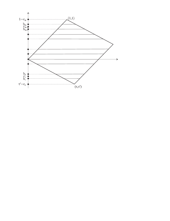
Let b1<b2<<bMsubscript𝑏1subscript𝑏2subscript𝑏𝑀b_{1}<b_{2}<\cdots<b_{M} be the projections onto internal space of the boundary cutting points of {(t,0): 0tR}conditional-set𝑡0 0𝑡𝑅\{(t,0)\ :\ 0\leq t\leq R\}. Define

c0=τ,c1=b1+b22,,cM1=bM1+bM2,cM=1.formulae-sequencesubscript𝑐0superscript𝜏formulae-sequencesubscript𝑐1subscript𝑏1subscript𝑏22formulae-sequencesubscript𝑐𝑀1subscript𝑏𝑀1subscript𝑏𝑀2subscript𝑐𝑀1\displaystyle c_{0}=\tau^{\prime},\ c_{1}=\tfrac{b_{1}+b_{2}}{2},\dots,\ c_{M-1}=\tfrac{b_{M-1}+b_{M}}{2},\ c_{M}=1\,.

The strips Sisubscript𝑆𝑖S_{i} formed by passing the interval [ci1,ci)subscript𝑐𝑖1subscript𝑐𝑖[c_{i-1},c_{i}) in internal space through C𝐶C in the direction of the physical axis, form a partition of C𝐶C. Through each strip in C𝐶C runs a part lisubscript𝑙𝑖l_{i} of our line {(t,0)L:0tR}conditional-setsubscript𝑡0𝐿0𝑡𝑅\{(t,0)_{L}:0\leq t\leq R\}. The idea is to use the intervals [ci1,ci)subscript𝑐𝑖1subscript𝑐𝑖[c_{i-1},c_{i}) as windows and the line segments lisubscript𝑙𝑖l_{i} as (part of) the physical space for a model set construction based on the lattice LN~~subscript𝐿𝑁\widetilde{L_{N}}. This will then produce the points on lisubscript𝑙𝑖l_{i} which will be our data points for the evaluation of the functions G~~𝐺\widetilde{G}, and then g𝑔g. In other words, we are implicitly using the partial model sets ΛLN~(Si)lisubscriptΛ~subscript𝐿𝑁subscript𝑆𝑖subscript𝑙𝑖\Lambda_{\widetilde{L_{N}}}(S_{i})\cap l_{i}.

Let m(R):=max{|cici1|}assign𝑚𝑅subscript𝑐𝑖subscript𝑐𝑖1m(R):=\max\{\left|c_{i}-c_{i-1}\right|\} and

εN:=supisup(x,v),(x,u)Si|G~(x,v)G~(x,u)|,i=1,,M.formulae-sequenceassignsubscriptsuperscript𝜀𝑁subscriptsupremum𝑖subscriptsupremum𝑥𝑣𝑥𝑢subscript𝑆𝑖~𝐺𝑥𝑣~𝐺𝑥𝑢𝑖1𝑀\displaystyle\varepsilon^{\prime}_{N}:=\sup_{i}\sup_{(x,v),(x,u)\in S_{i}}\left|\widetilde{G}(x,v)-\widetilde{G}(x,u)\right|\,,\qquad i=1,\dots,M\,.
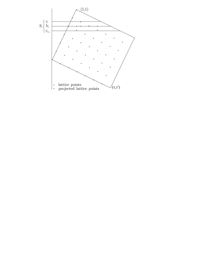
Refer to caption
Figure 5. The projections b1,,bMsubscript𝑏1subscript𝑏𝑀b_{1},\dots,b_{M} into internal space of the boundary cutting points of the path. The points c0,,cMsubscript𝑐0subscript𝑐𝑀c_{0},\dots,c_{M} mark the boundaries of the smaller windows into which the original window [τ,1)superscript𝜏1[\tau^{\prime},1) is partitioned.

Each s~jS~subscript~𝑠𝑗~𝑆\tilde{s}_{j}\in\widetilde{S} lies in exactly one strip Sisubscript𝑆𝑖S_{i}. Let (pj,qj)subscript𝑝𝑗subscript𝑞𝑗(p_{j},q_{j}) be its projection onto the line segment lisubscript𝑙𝑖l_{i}. Then (pj,qj)(uj,0)Lsubscript𝑝𝑗subscript𝑞𝑗subscriptsubscript𝑢𝑗0𝐿(p_{j},q_{j})\equiv(u_{j},0)_{L} for some uj[0,R]subscript𝑢𝑗0𝑅u_{j}\in[0,R]. Thus we obtain {(u1,0),,(uN2,0)}subscript𝑢10subscript𝑢superscript𝑁20\{(u_{1},0),\dots,(u_{N^{2}},0)\} on our path {(t,0)L: 0tR}conditional-setsubscript𝑡0𝐿 0𝑡𝑅\{(t,0)_{L}\,:\,0\leq t\leq R\}.

Refer to caption
Figure 6. The points s~jsubscript~𝑠𝑗\tilde{s}_{j} lying in the strip Sisubscript𝑆𝑖S_{i} formed by the window [ci1,ci)subscript𝑐𝑖1subscript𝑐𝑖[c_{i-1},c_{i}) are projected onto the segment lisubscript𝑙𝑖l_{i} of the path {(t,0)L:0tR}conditional-setsubscript𝑡0𝐿0𝑡𝑅\{(t,0)_{L}:0\leq t\leq R\} producing data points ujsubscript𝑢𝑗u_{j}, shown here as small crosses.

We have the estimate (38). Moreover,

5N2i=1N2G~(s~i)=5N2i=1N2(G~(s~i)G~(pi,qi))+5N2i=1N2g(ui),5superscript𝑁2superscriptsubscript𝑖1superscript𝑁2~𝐺subscript~𝑠𝑖5superscript𝑁2superscriptsubscript𝑖1superscript𝑁2~𝐺subscript~𝑠𝑖~𝐺subscript𝑝𝑖subscript𝑞𝑖5superscript𝑁2superscriptsubscript𝑖1superscript𝑁2𝑔subscript𝑢𝑖\displaystyle\frac{\sqrt{5}}{{N^{2}}}\sum_{i=1}^{N^{2}}\widetilde{G}(\tilde{s}_{i})=\frac{\sqrt{5}}{{N^{2}}}\sum_{i=1}^{N^{2}}(\widetilde{G}(\tilde{s}_{i})-\widetilde{G}(p_{i},q_{i}))+\frac{\sqrt{5}}{{N^{2}}}\sum_{i=1}^{N^{2}}g(u_{i})\,,

since

G~(pi,qi)=G~((ui,0))=g(ui).~𝐺subscript𝑝𝑖subscript𝑞𝑖~𝐺subscript𝑢𝑖0𝑔subscript𝑢𝑖\displaystyle\widetilde{G}(p_{i},q_{i})=\widetilde{G}((u_{i},0))=g(u_{i})\,.

Thus

|5N2i=1N2G~(s~i)5N2i=1N2g(ui)|5N2i=1N2εN=5εN,5superscript𝑁2superscriptsubscript𝑖1superscript𝑁2~𝐺subscript~𝑠𝑖5superscript𝑁2superscriptsubscript𝑖1superscript𝑁2𝑔subscript𝑢𝑖5superscript𝑁2superscriptsubscript𝑖1superscript𝑁2subscriptsuperscript𝜀𝑁5subscriptsuperscript𝜀𝑁\left|\frac{\sqrt{5}}{{N^{2}}}\sum_{i=1}^{N^{2}}\widetilde{G}(\tilde{s}_{i})-\frac{\sqrt{5}}{{N^{2}}}\sum_{i=1}^{N^{2}}g(u_{i})\right|\leq\frac{\sqrt{5}}{{N^{2}}}\sum_{i=1}^{N^{2}}\varepsilon^{\prime}_{N}=\sqrt{5}\,\varepsilon^{\prime}_{N}\,, (39)

since s~isubscript~𝑠𝑖\tilde{s}_{i} and (pi,qi)subscript𝑝𝑖subscript𝑞𝑖(p_{i},q_{i}) both have second component in the same interval [ci1,ci)subscript𝑐𝑖1subscript𝑐𝑖[c_{i-1},c_{i}).

Combining (38) and (39), we have

|𝕋G~𝑑θ5N2i=1N2g(ui)|<5(εN+εN).subscript𝕋~𝐺differential-d𝜃5superscript𝑁2superscriptsubscript𝑖1superscript𝑁2𝑔subscript𝑢𝑖5subscript𝜀𝑁subscriptsuperscript𝜀𝑁\left|\int_{\mathbb{T}}\widetilde{G}\,d\theta-\frac{\sqrt{5}}{{N^{2}}}\sum_{i=1}^{N^{2}}g(u_{i})\right|<\sqrt{5}\,(\varepsilon_{N}+\varepsilon^{\prime}_{N})\,. (40)

This provides a method of estimating the integral 𝕋G~𝑑θsubscript𝕋~𝐺differential-d𝜃\int_{\mathbb{T}}\widetilde{G}\,d\theta using only g𝑔g on [0,R]0𝑅[0,R] along with well chosen points in the interval. The two parameters N𝑁N and R𝑅R control the estimates.

In spite of the apparent complexity of strips, what is going on is easy to implement. For each s~i=(si,si)subscript~𝑠𝑖subscript𝑠𝑖subscriptsuperscript𝑠𝑖\tilde{s}_{i}=(s_{i},s^{\prime}_{i}) there is a translation vector t~jT~subscript~𝑡𝑗~𝑇\tilde{t}_{j}\in\tilde{T} for which |si+tj|subscriptsuperscript𝑠𝑖subscriptsuperscript𝑡𝑗|s^{\prime}_{i}+t^{\prime}_{j}| is minimal. The corresonding data point is then ui:=si+tjassignsubscript𝑢𝑖subscript𝑠𝑖subscript𝑡𝑗u_{i}:=s_{i}+t_{j}. This is Step 5 of §4.2.

6. Two explicit examples

6.1. Computation of Fourier coefficients

In this section we apply the methods outlined above to two almost periodic functions f::𝑓f:\mathbb{R}\rightarrow\mathbb{R}, both local with respect to the model set Λ=Λ([1,1τ))ΛΛ11𝜏\Lambda=\Lambda([-1,\tfrac{1}{\tau})) of §5.3. The first is the distance-to-the-nearest neighbour function

f(t)=the distance of t to the nearest point of Λ.𝑓𝑡the distance of t to the nearest point of Λf(t)=\textrm{the distance of $t$ to the nearest point of $\Lambda$}\,. (41)

This is a continuous and piecewise linear function that is local with respect to ΛΛ\Lambda.

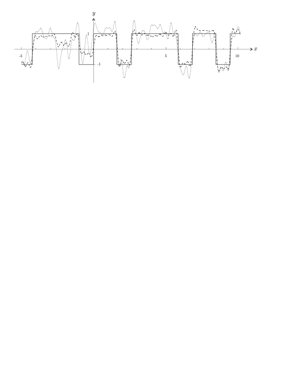
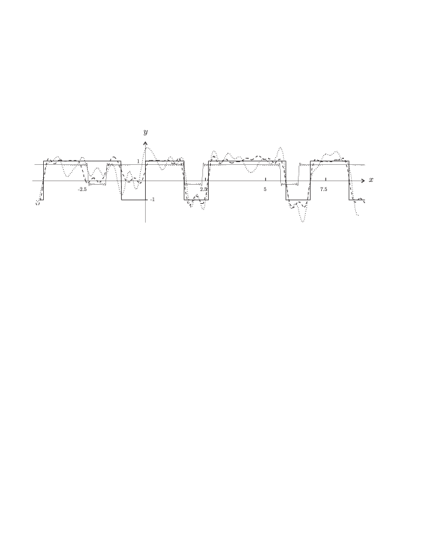
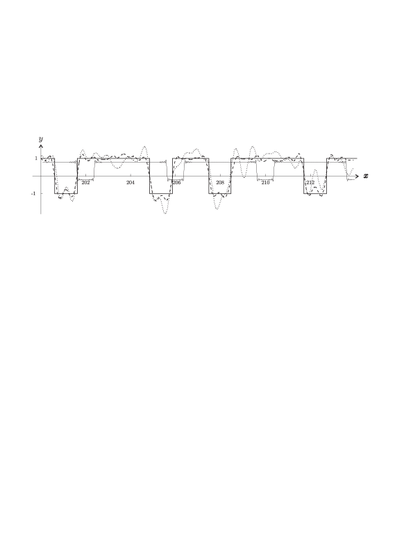
The second is the function

f:f(x)={1,if x is in a long interval1,if x is in a short interval,f:\quad f(x)=\begin{cases}1,&\text{if $x$ is in a long interval}\\ -1,&\text{if $x$ is in a short interval}\,,\end{cases} (42)

which local, but only piecewise continuous with breaks wherever x𝑥x switches from a long to a short interval.

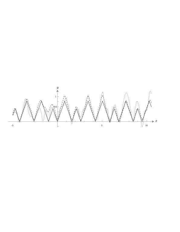
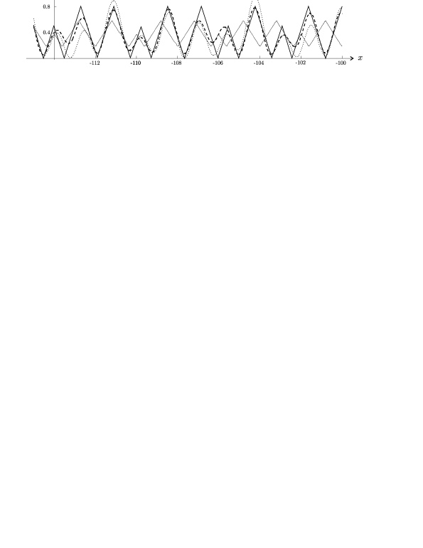
Graphs of these functions are shown (solid lines) in Fig. 8 and Fig. 13 respectively.

Our objective is to see how well the approximations we have discussed compare with the actual functions when the calculations are done with specific choices of data points.

We approximate each of the two functions by a finite number of terms of its Fourier-Bohr expansion (18), which in our setting here reads:

f(x)=k~[τ]~ake2πi(k|x),x.formulae-sequence𝑓𝑥subscript~𝑘~superscriptdelimited-[]𝜏subscript𝑎𝑘superscript𝑒2𝜋𝑖conditional𝑘𝑥𝑥\displaystyle f(x)=\sum_{\tilde{k}\in\widetilde{\mathbb{Z}[\tau]^{\circ}}}a_{k}e^{2\pi i(k|x)}\,,\qquad x\in\mathbb{R}\,. (43)

For the two functions f𝑓f chosen here, it is easy to determine the corresponding functions F~~𝐹\tilde{F} on the torus 𝕋=(×)/L~𝕋~𝐿\mathbb{T}=(\mathbb{R}\times\mathbb{R})/\widetilde{L} and hence to compute the Fourier-Bohr coefficients aksubscript𝑎𝑘a_{k} exactly by (19), see §6.2 . For the nearest neighbour function these are given explicitly in (50).

On the other hand, the approximation depends on the choice of the refinement lattice LN~~subscript𝐿𝑁\widetilde{L_{N}}, which shall here always be of the form (1/N)L~=(1/N)[τ]~1𝑁~𝐿1𝑁~delimited-[]𝜏(1/N)\widetilde{L}=(1/N)\widetilde{\mathbb{Z}[\tau]} (so the index [LN~:L~]delimited-[]:~subscript𝐿𝑁~𝐿[\widetilde{L_{N}}:\widetilde{L}] is N2superscript𝑁2N^{2}). This determines both the points that will eventually be projected into our data points and also the values of k𝑘k which shall be included in approximating the sum (43), namely a set K~~𝐾\tilde{K} of k~=(k,k)[τ]~~𝑘𝑘superscript𝑘superscript~delimited-[]𝜏\tilde{k}=(k,k^{\prime})\in\widetilde{\mathbb{Z}[\tau]}^{\circ} chosen as representatives of the group [τ]~/N[τ]~superscript~delimited-[]𝜏𝑁superscript~delimited-[]𝜏\widetilde{\mathbb{Z}[\tau]}^{\circ}/N\widetilde{\mathbb{Z}[\tau]}^{\circ} dual to the group ((1/N)[τ]~)/L~1𝑁~delimited-[]𝜏~𝐿((1/N)\widetilde{\mathbb{Z}[\tau]})/\widetilde{L}. Our choice is take the k~~𝑘\tilde{k} with |k|𝑘|k| as small as possible, so K𝐾K consists of elements k[τ]𝑘delimited-[]𝜏k\in\mathbb{Z}[\tau], one for each congruence class of [τ]delimited-[]𝜏\mathbb{Z}[\tau] modulo N[τ]𝑁delimited-[]𝜏N\mathbb{Z}[\tau], chosen so that |k|𝑘|k| is minimal in its class. We denote by fexact(x)superscript𝑓𝑒𝑥𝑎𝑐𝑡𝑥f^{exact}(x) the finite series, taken from (43), approximating f(x)𝑓𝑥f(x), x𝑥x\in\mathbb{R}:

fexact(x)=kKake2πi(k|x),x.formulae-sequencesuperscript𝑓𝑒𝑥𝑎𝑐𝑡𝑥subscript𝑘𝐾subscript𝑎𝑘superscript𝑒2𝜋𝑖conditional𝑘𝑥𝑥f^{exact}(x)=\sum_{k\in K}a_{k}e^{2\pi i(k|x)}\,,\qquad x\in\mathbb{R}\,. (44)

Next we replace the coefficients aksubscript𝑎𝑘a_{k} in fexact(x)superscript𝑓𝑒𝑥𝑎𝑐𝑡𝑥f^{exact}(x) by their approximations

akint:=1R0Rf(x)e2πi(k|x)dxassignsuperscriptsubscript𝑎𝑘𝑖𝑛𝑡1𝑅superscriptsubscript0𝑅𝑓𝑥superscript𝑒2𝜋𝑖conditional𝑘𝑥differential-d𝑥\displaystyle a_{k}^{int}:=\frac{1}{R}\int_{0}^{R}f(x)e^{-2\pi i(k|x)}{\rm d}x (45)

following from (22), and denote the resulting function by fint(x)superscript𝑓𝑖𝑛𝑡𝑥f^{int}(x). We shall use various values of R𝑅R, all of which correspond to a set of complete passes across the fundamental region, as illustrated in Fig. 5.

The integrals (45) are to be estimated by reducing them to finite sums where the integrand is computed on the finite set of data arising as projections {u1,,uN2}subscript𝑢1subscript𝑢superscript𝑁2\{u_{1},\dots,u_{N^{2}}\} of the N2superscript𝑁2N^{2} points in C𝐶C, as explained in §4.3:

aksum:=1N2j=1N2f(uj)e2πi(k|uj).assignsuperscriptsubscript𝑎𝑘𝑠𝑢𝑚1superscript𝑁2superscriptsubscript𝑗1superscript𝑁2𝑓subscript𝑢𝑗superscript𝑒2𝜋𝑖conditional𝑘subscript𝑢𝑗\displaystyle a_{k}^{sum}:=\frac{1}{N^{2}}\sum_{j=1}^{N^{2}}f(u_{j})e^{-2\pi i(k|u_{j})}. (46)

The resulting approximation to fexact(x)superscript𝑓𝑒𝑥𝑎𝑐𝑡𝑥f^{exact}(x) is denoted fsum(x)superscript𝑓𝑠𝑢𝑚𝑥f^{sum}(x). This is the approximation that we have been working towards. Written out in full it reads:

fsum(x)=kK{1N2j=1N2f(uj)e2πi(k|uj)}e2πi(k|x).superscript𝑓𝑠𝑢𝑚𝑥subscript𝑘𝐾1superscript𝑁2superscriptsubscript𝑗1superscript𝑁2𝑓subscript𝑢𝑗superscript𝑒2𝜋𝑖conditional𝑘subscript𝑢𝑗superscript𝑒2𝜋𝑖conditional𝑘𝑥f^{sum}(x)=\sum_{k\in K}\,\left\{\frac{1}{N^{2}}\sum_{j=1}^{N^{2}}f(u_{j})e^{-2\pi i(k|u_{j})}\right\}\,e^{2\pi i(k|x)}\,. (47)

It is computed out of data points in \mathbb{R}, is a finite sum of exponential functions whose frequencies come from the Fourier module of f𝑓f, and utilizes discrete groups arising out of the periodic setting of the underlying cut and project scheme. By its form, fsumsuperscript𝑓𝑠𝑢𝑚f^{sum} is almost periodic and approximates the function F~~𝐹\tilde{F} everywhere on the real line as it lies wrapped around the torus.

Thus we have four functions: f,fexact,fint,fsum𝑓superscript𝑓𝑒𝑥𝑎𝑐𝑡superscript𝑓𝑖𝑛𝑡superscript𝑓𝑠𝑢𝑚f,\;f^{exact},\;f^{int},\;f^{sum}, all defined for all x𝑥x\in\mathbb{R}. The three approximation functions depend on the number M𝑀M of passes of the real line going through the fundamental region C𝐶C (see § 5.4 and 5.5 for details), and on the number N2superscript𝑁2N^{2} of lattice points of LN~~subscript𝐿𝑁\widetilde{L_{N}} found in C𝐶C. Each of them restricts the full summation of the Fourier-Bohr expansion to the same finite set K𝐾K of frequencies. They differ due to the ways in which the Fourier-Bohr coefficients are obtained: they are exact in the first case (or at least as exact as real computation on computers can be), are derived from the integral approximation in the second, and come from the finite sum approximation to the integral in the third. The calculations and graphs shown below allow one to compare these functions. The exact coefficients and their approximations by integrals are sufficiently close as to make little difference to the graphs, so the figures are restricted to comparing f,fint,fsum𝑓superscript𝑓𝑖𝑛𝑡superscript𝑓𝑠𝑢𝑚f,f^{int},f^{sum}.

By way of comparison, there is one further Fourier approximant, of the type that we are obtained by periodically extending f𝑓f from its values on a fixed finite interval I𝐼I of \mathbb{R} to the entire space \mathbb{R}. Thus we introduce

fcos(x)=k=0nakcos(12kπx),whereak=1202f(x)cos(12kπx)dx.formulae-sequencesuperscript𝑓𝑐𝑜𝑠𝑥superscriptsubscript𝑘0𝑛subscript𝑎𝑘12𝑘𝜋𝑥wheresubscript𝑎𝑘12superscriptsubscript02𝑓𝑥12𝑘𝜋𝑥differential-d𝑥\displaystyle f^{cos}(x)=\sum_{k=0}^{n}a_{k}\cos(\frac{1}{2}{k\pi x}),\qquad\text{where}\qquad a_{k}=\frac{1}{2}\int_{0}^{2}f(x)\cos(\frac{1}{2}{k\pi x}){\rm d}x\,. (48)

Needless to say, fcossuperscript𝑓𝑐𝑜𝑠f^{cos} cannot be expected to have much relationship to f𝑓f outside I𝐼I, and it doesn’t. In fact, fcossuperscript𝑓𝑐𝑜𝑠f^{cos} does not appear to be a good choice even on the limited domain I𝐼I.

6.2. Computing the exact Fourier-Bohr coefficients

It may be of interest to indicate how we computed the exact Fourier-Bohr coefficients. We can reorganize Fig. 3, translating the a𝑎a and b𝑏b regions into single blocks (see Fig. 7), a procedure that is familiar from the klotz construction see §§\S7 often used in studying cut and project sets, [13].

It is then straightforward to understand the corresponding function F~~𝐹\tilde{F} on the 2-dimensional torus, i.e. a genuinely periodic function for which f(t)=F~(t,0)mod[τ]~𝑓𝑡modulo~𝐹𝑡0~delimited-[]𝜏f(t)=\widetilde{F}(t,0)\mod{\widetilde{\mathbb{Z}[\tau]}}.

Refer to caption
Figure 7. The a𝑎a and b𝑏b regions of Fig. 3 are reorganized here into two rectangles (heavy lines). The function F~~𝐹\widetilde{F} on 𝕋𝕋\mathbb{T} arising from the local function (41) is supported on these two rectangles. It is constant on vertical lines. Along the horizontal axis, on the b𝑏b rectangle the function values start at 00, increase linearly to 1/2121/2 at the mid point of the rectangle and then linearly decrease to 00 again. Similarly on the a𝑎a rectangle they increase to τ/2𝜏2\tau/2 and then return to 00.

Furthermore, it is easy to compute the ‘exact’ Fourier coefficients of F~~𝐹\widetilde{F}. Let k~=aω~1+bω~2[τ]~~𝑘𝑎subscript~𝜔1𝑏subscript~𝜔2superscript~delimited-[]𝜏\widetilde{k}=a\widetilde{\omega}_{1}+b\widetilde{\omega}_{2}\in\widetilde{\mathbb{Z}[\tau]}^{\circ}, where a,b𝑎𝑏a,b\in\mathbb{Z}. Then

(k~(x,y))=x(k~(1,0))+y(k~(0,1))=2xkδ+2ykδ,conditional~𝑘𝑥𝑦𝑥conditional~𝑘10𝑦conditional~𝑘012𝑥𝑘𝛿2𝑦superscript𝑘superscript𝛿\displaystyle(\widetilde{k}\mid(x,y))=x\,(\widetilde{k}\mid(1,0))+y\,(\widetilde{k}\mid(0,1))=2xk\delta+2yk^{\prime}\delta^{\prime}\,,

where

k=a+bτ2,k=a+bτ2.formulae-sequence𝑘𝑎𝑏𝜏2superscript𝑘𝑎𝑏superscript𝜏2\displaystyle k=\frac{a+b\tau}{2}\,,\qquad k^{\prime}=\frac{a+b\tau^{\prime}}{2}\,.

The Fourier coefficient for k~~𝑘\widetilde{k} is

ak=𝕋F~(w)e2πi(k~w)𝑑w=0101F~(u,v)e2πi(k~u1~+vτ~)𝑑u𝑑v.subscript𝑎𝑘subscript𝕋~𝐹𝑤superscript𝑒2𝜋𝑖conditional~𝑘𝑤differential-d𝑤superscriptsubscript01superscriptsubscript01~𝐹𝑢𝑣superscript𝑒2𝜋𝑖conditional~𝑘𝑢~1𝑣~𝜏differential-d𝑢differential-d𝑣a_{k}=\int_{\mathbb{T}}\widetilde{F}(w)\,e^{-2\pi i(\widetilde{k}\mid w)}\,dw=\int_{0}^{1}\int_{0}^{1}\widetilde{F}(u,v)\,e^{-2\pi i(\widetilde{k}\mid u\widetilde{1}+v\widetilde{\tau})}\,du\,dv\,. (49)

Writing

u1~+vτ~=(u+vτ,u+vτ)=:(x,y),\displaystyle u\widetilde{1}+v\widetilde{\tau}=(u+v\tau,u+v\tau^{\prime})=:(x,y)\,,

we have

(k~u1~+vτ~)=2kxδ+2kyδ.conditional~𝑘𝑢~1𝑣~𝜏2𝑘𝑥𝛿2superscript𝑘𝑦superscript𝛿\displaystyle(\widetilde{k}\mid u\widetilde{1}+v\widetilde{\tau})=2kx\delta+2k^{\prime}y\delta^{\prime}\,.

Making the change from the variables u𝑢u and v𝑣v to x𝑥x and y𝑦y, and using the definition of F~~𝐹\widetilde{F}, we obtain

aksubscript𝑎𝑘\displaystyle a_{k} =\displaystyle= 151τ010(12|x+12|)e4πi(kxδ+kyδ)𝑑x𝑑y15superscriptsubscript1𝜏0superscriptsubscript1012𝑥12superscript𝑒4𝜋𝑖𝑘𝑥𝛿superscript𝑘𝑦superscript𝛿differential-d𝑥differential-d𝑦\displaystyle\frac{1}{\sqrt{5}}\int_{-\tfrac{1}{\tau}}^{0}\int_{-1}^{0}\left(\frac{1}{2}-\left|x+\frac{1}{2}\right|\right)e^{-4\pi i(kx\delta+k^{\prime}y\delta^{\prime})}\;dx\;dy (50)
+\displaystyle+ 151τ1τ20τ(τ2|xτ2|)e4πi(kxδ+kyδ)𝑑x𝑑y.15superscriptsubscript1𝜏1superscript𝜏2superscriptsubscript0𝜏𝜏2𝑥𝜏2superscript𝑒4𝜋𝑖𝑘𝑥𝛿superscript𝑘𝑦superscript𝛿differential-d𝑥differential-d𝑦\displaystyle\frac{1}{\sqrt{5}}\int_{-\tfrac{1}{\tau}}^{\tfrac{1}{\tau^{2}}}\int_{0}^{\tau}\left(\frac{\tau}{2}-\left|x-\frac{\tau}{2}\right|\right)e^{-4\pi i(kx\delta+k^{\prime}y\delta^{\prime})}\;dx\;dy\,.

Note that the factor 1515\tfrac{1}{\sqrt{5}} comes from x=u+vτ𝑥𝑢𝑣𝜏x=u+v\tau, y=u+vτ𝑦𝑢𝑣superscript𝜏y=u+v\tau^{\prime}.

|1τ1τ|=ττ=5.matrix1𝜏1superscript𝜏superscript𝜏𝜏5\displaystyle\left|\begin{matrix}1&\tau\\ 1&\tau^{\prime}\end{matrix}\right|=\tau^{\prime}-\tau=-\sqrt{5}.

6.3. Shadows of singularities

Inspection of the aperiodic approximations shows that they are remarkably faithful to the originals. But there is apparently a strange fuzziness in the approximation in the interval [τ2,0]superscript𝜏20[-\tau^{2},0]. The explanation for this is quite interesting and shows that the approximation method we use here is sensitive to quite subtle qualities of the aperiodicity.

The particular Fibonacci set that we have used in our example is singular, that is to say, it is one at which the torus parametrization is not one-one. As pointed out in footnote of 4, ΛΛ\Lambda is but one of two distinct sets in X(Λ)𝑋ΛX(\Lambda) that map to the same point on the torus 𝕋𝕋\mathbb{T} under the torus map. The other one differs from ΛΛ\Lambda only in that it contains {τ}𝜏\{-\tau\} but not {1}1\{-1\}. The Fourier analysis takes place on 𝕋𝕋\mathbb{T} and treats these two sets equally. However the nearest neighbour functions of the two sets are different. This is a difference that it immaterial to F~~𝐹\tilde{F}, which our function fsumsuperscript𝑓𝑠𝑢𝑚f^{sum} is approximating, but which the original function F𝐹F can see. What we see is the Fourier analysis hedging between the two scenarios.

Further refinements of the lattice will never improve the situation on this interval. However, if we had used an element of X(Λ)𝑋ΛX(\Lambda) at which the torus map were 11111-1 (and this is the case with probabilistic certainty if one chooses randomly from X(Λ)𝑋ΛX(\Lambda)) then this phenomenon would not occur and the approximation would be uniformly valid over the entire space. All one need do is to shift the window so that its end points do not lie in the set [τ]delimited-[]𝜏\mathbb{Z}[\tau], e.g. 12+[1,1τ]1211𝜏\frac{1}{2}+[-1,\frac{1}{\tau}].


7. Final Comments

We should point out that there is considerable scope for adapting the scenario sketched out here. It is possible to arrange things so that they are related to tilings. One elegant tiling method is the klotz construction [13, 14]. One begins with the decomposition into Voronoi cells of the lattice L~~𝐿\widetilde{L} in d×dsuperscript𝑑superscript𝑑\mathbb{R}^{d}\times\mathbb{R}^{d}, and along with it the corresponding dual cell decomposition into Delone cells. For each pair of P,Q𝑃𝑄P,Q consisting of intersecting d𝑑d-dimensional faces P𝑃P and Q𝑄Q from a Voronoi cell and a Delone cell respectively, form the klotz P||×QP^{||}\times Q^{\perp} in d×dsuperscript𝑑superscript𝑑\mathbb{R}^{d}\times\mathbb{R}^{d}. The set of these klötze form a tiling of d×dsuperscript𝑑superscript𝑑\mathbb{R}^{d}\times\mathbb{R}^{d}. Furthermore the intersection of (d,0)superscript𝑑0(\mathbb{R}^{d},0) with this tiling produces a tiling of physical space. (If one chooses instead to do the projections the other way around, one gets a different tiling). Several of these klötze can be combined to form a fundamental region for d×dsuperscript𝑑superscript𝑑\mathbb{R}^{d}\times\mathbb{R}^{d}, as we see in Fig. 7, and this type of choice should lead to computational methods that are adapted to the these tilings. For instance, the region A𝐴A of integration might well be chosen as the union of a finite number of tiles. For more on determining Voronoi and Delone cells in the context of high symmetry, see [19].

The method advocated here is based on the idea of local functions, the extending of them into the context of compact Abelian groups, and the discretization of the resulting Fourier analysis by the use of finite groups. In the 1D setting that was explored in detail here, the only symmetries involved arise from translational symmetry (which is at the base of the almost periodicity). In higher dimensions, especially those of interest to the quasicrystal community, decagonal, icosahedral, or other symmetries appear. In these cases there are a number of ways of utilizing the symmetry to greatly improve the efficiency of the computation, in the same spirit as [18]. As we have pointed out, the preparations required for this depend largely on the cut and project scheme and not so much on the actual model set involved. Fortunately the cut and project schemes for these settings are essentially canonical and their strong algebraic nature makes this program quite feasible.

Finally, although we have not spelled it out here, the way in which finite groups and their duals are used here makes the process amenable to the technique of the fast Fourier transform. Details will appear later.

Acknowledgements

Work supported in part by the Natural Sciences and Engineering Research Council of Canada, the MIND Research Institute of Santa Ana, Calif., the Aspen Center for Physics, and MITACS. The authors are grateful to the referees for their constructive comments.

References

  • [1] L. Amerio and G. Prouse Almost-periodic functions and functional equations, Litton Educational Publishing, New York 1971.
  • [2] M. Baake, D. Lenz, and R.V. Moody, Characterisation of models sets by dynamical systems, Ergodic Th. & Dynam. Syst. 27 (2007) 341–382; arXiv:math.DS/0511648.
  • [3] A. S. Besicovitch, Almost periodic functions, Dover publications, Cambrige 1954.
  • [4] S. Bochner, Properties of Fourier series of almost periodic functions, Proc. London Math. Soc. 26 (1927) 433-452.
  • [5] S. Bochner, A new approach to almost periodicity, Proceedings of the Nat. Acad. Sci. USA 48 (1962) 195-205.
  • [6] S. Bochner, J. von Neumann, Almost periodic functions of groups II, Trans. Am. Math. Soc. 37 (1935) 21-50.
  • [7] H. Bohr, Almost periodic functions, Chelsea publishing company, 1947.
  • [8] P. Bohl, Über die Darstellung von Funktionen einer Variabeln durch trigonometrische Reihen mit mehreren einer Variabeln proportionalen Argumenten , Dorpat (1893) (Thesis).
  • [9] R.B. Burckel, Weakly almost periodic functions on semigroups, Gordon & Breach, Science Publishers, New York 1970.
  • [10] L. Chen, R. V. Moody, and J. Patera, Non-crystallographic root systems, in Quasicrystals and Discrete Geometry, Fields Institute Monograph Series 10 (1998) 135–178, ed. J. Patera, Amer. Math. Soc.
  • [11] A. Hof, On diffraction by aperiodic structures, Commun. Math. Phys. 169 (1995) 25–43.
  • [12] Gerhard Keller, Equilibrium states in ergodic theory, LMS Student Texts, 42, Cambridge U. Press, Cambridge 1998.
  • [13] P. Kramer, Atomic order in quasicrystals is supported by several unit cells, Mod. Phys. Lett. B1(1987) 7-18.
  • [14] P. Kramer and M. Schlottmann, Dualization of Voronoi domains and klotz construction: a general method for the generation of proper space filling, J. Phys. A22(1989) L1097-L1102.
  • [15] B.M. Levitan and V.V. Zhikov Almost periodic functions and differential equations, Cambridge University Press, Cambridge 1982.
  • [16] Yves Meyer, Algebraic numbers and harmonic analysis, North-Holland Publ., Amsterdam - London, 1972.
  • [17] R. V. Moody, Model sets and their duals, in The mathematics of long-range order, ed. R.V. Moody, NATO ASI, Series C489, Kluwer, Dordrecht (1997) 239-268.
  • [18] R. V. Moody and J. Patera, Characters of elements of finite order in Lie groups, SIAM Journal for Algebraic and Discrete Methods, 5 (1984) 359-383.
  • [19] R. V. Moody and J. Patera, Voronoi domains and dual cells in the generalized kaleidoscope with applications to root and weight lattices, Can. J. Math., 47 (1995) 573–605.
  • [20] R.V. Moody and J. Patera, Orthogonality within the families of C𝐶C-, S𝑆S-, and E𝐸E-functions of any compact semisimple Lie group, SIGMA (Symmetry, Integrability and Geometry: Methods and Applications) 2 (2006) 076, 14 pages, math-ph/0611020.
  • [21] C. Radin and M. Wolf, Space tilings and local isomorphism, Geometriae Dedicata 42 (1992) 355-360.
  • [22] M. Schlottmann, Generalized model sets and dynamical systems, in Directions in mathematical quasicrystals eds. M. Baake and R. Moody, CRM monograph series vol. 13 AMS Providence RI (2000) pp. 143-159.
  • [23] H. Weyl, Integralgleichungen und fastperiodische Funktionen, Math. Ann. 97 (1926-7) 473-498.
  • [24] N. Wiener, On the representation of functions by trigonometrical integrals, Math. Zeitschr. 24 (1926) 575-616.

R.V. Moody: Department of Mathematics, University of Victoria, Victoria, British Columbia, Canada; rmoody@uvic.ca.

M. Nesterenko: Institute of Mathematics, NAS of Ukraine, 3 Tereshchenkivs’ka Street, Kyiv-4, 01601, Ukraine; maryna@imath.kiev.ua.

J. Patera: Centre de recherches mathématiques, Université de Montréal, C.P.6128-Centre ville, Montréal, H3C 3J7, Québec, Canada; patera@crm.umontreal.ca.

Appendix A Numerical and graphical data for two exact examples of section 6, i.e., the distance-to-the-nearest neighbour function given in (41) and the local function defined by (42)


Table 1. Comparison of the calculated coefficients aksubscript𝑎𝑘a_{k} in the approximations fexactsuperscript𝑓𝑒𝑥𝑎𝑐𝑡f^{exact}, fintsuperscript𝑓𝑖𝑛𝑡f^{int}, and fsumsuperscript𝑓𝑠𝑢𝑚f^{sum} based on the parameters of Fig. 10.
k𝑘k akexactsuperscriptsubscript𝑎𝑘𝑒𝑥𝑎𝑐𝑡a_{k}^{exact} akintsuperscriptsubscript𝑎𝑘𝑖𝑛𝑡a_{k}^{int} aksumsuperscriptsubscript𝑎𝑘𝑠𝑢𝑚a_{k}^{sum}
1212τ1212𝜏-\frac{1}{2}-\frac{1}{2}\tau -0.1065-0.03668i -0.1065-0.0371i -0.1086-0.0581i
1212-\frac{1}{2} 0.0243+0.0287i 0.0236+0.0292i 0.0269+0.0711i
12+12τ1212𝜏-\frac{1}{2}+\frac{1}{2}\tau 0.0026+0.0153i 0.0035+0.0155i 0.0233-0.0332i
12τ12𝜏-\frac{1}{2}\tau -0.0683+0.0407i -0.0680+0.0412i -0.0517+0.0542i
00 0.3618 0.3618 0.3367
12τ12𝜏\frac{1}{2}\tau -0.0683-0.0407i -0.0680-0.0412i -0.0517-0.0542i
1212τ1212𝜏\frac{1}{2}-\frac{1}{2}\tau 0.0026-0.0153i 0.0035-0.0155i 0.0233+0.0332i
1212\frac{1}{2} 0.0243-0.0287i 0.0236-0.0292i 0.0269-0.0711i
12+12τ1212𝜏\frac{1}{2}+\frac{1}{2}\tau -0.1065+0.0367i -0.1065+0.0371i -0.1086+0.0581i
Table 2. Comparison of the values of the function f𝑓f of (41) and its approximants fexactsuperscript𝑓𝑒𝑥𝑎𝑐𝑡f^{exact}, fintsuperscript𝑓𝑖𝑛𝑡f^{int}, fsumsuperscript𝑓𝑠𝑢𝑚f^{sum}, and fcossuperscript𝑓𝑐𝑜𝑠f^{cos}, see Fig. 10.
xisubscript𝑥𝑖x_{i} f(xi)𝑓subscript𝑥𝑖f(x_{i}) fexact(xi)superscript𝑓𝑒𝑥𝑎𝑐𝑡subscript𝑥𝑖f^{exact}(x_{i}) fint(xi)superscript𝑓𝑖𝑛𝑡subscript𝑥𝑖f^{int}(x_{i}) fsum(xi)superscript𝑓𝑠𝑢𝑚subscript𝑥𝑖f^{sum}(x_{i}) fcos(xi)superscript𝑓𝑐𝑜𝑠subscript𝑥𝑖f^{cos}(x_{i})
-100 0.8065 0.6916 0.6965 0.7728 0.1859
-50 0.4033 0.4229 0.4208 0.4562 0.3690
-15 0.3262 0.2555 0.2522 0.1461 0.4912
35τ35𝜏-3-5\tau 0 0.0577 0.0584 0.1378 0.5365
0 0 0.0658 0.0670 0.1165 0.1859
τ𝜏\tau 0 0.0797 0.0788 0.0946 0.1858
0.25+τ0.25𝜏0.25+\tau 0.2500 0.2060 0.2049 0.1995 0.3065
0.5+τ0.5𝜏0.5+\tau 0.5000 0.3318 0.3313 0.3416 0.3138
1+τ1𝜏1+\tau 0 0.1659 0.1649 0.1115 0.3000
1+1.25τ11.25𝜏1+1.25\tau 0.4045 0.3325 0.3287 0.1467 0.5022
1+2.5τ12.5𝜏1+2.5\tau 0.8090 0.6562 0.6609 0.6949 0.4681
1+2.75τ12.75𝜏1+2.75\tau 0.4045 0.3119 0.3152 0.2659 0.2659
50 0.4033 0.3265 0.3229 0.1209 0.3690
100 0.1885 0.3006 0.3004 0.2282 0.1859
500 0.4396 0.4669 0.4651 0.5364 0.1859
Refer to caption
Figure 8. The solid line is the graph of f𝑓f of (41). The dotted curve shows the fsumsuperscript𝑓𝑠𝑢𝑚f^{sum} approximation and the dashed curve shows the fintsuperscript𝑓𝑖𝑛𝑡f^{int} approximation. Both approximations were calculated using a total of N2=49superscript𝑁249N^{2}=49 lattice points in C𝐶C and M=11𝑀11M=11 path passes in C𝐶C, corresponding to an interval of integration R23,30𝑅2330R\approx 23,30.
Refer to caption
Figure 9. The function f𝑓f and approximants of (41) are drawn with the same conventions as in Fig. 8, but for refined parameters: M=17𝑀17M=17, N2=121superscript𝑁2121N^{2}=121, and R37,43𝑅3743R\approx 37,43. See subsection 6.3 for an explanation of the misfit of approximations in the region [τ2,0]superscript𝜏20[-\tau^{2},0].
Refer to caption
Figure 10. The function f𝑓f of (41) is graphed for parameters: N2=9superscript𝑁29N^{2}=9 lattice points from C𝐶C, M=10𝑀10M=10 passes of the fundamental domain, and corresponding interval of integration given by R21,64𝑅2164R\approx 21,64. Also the periodic approximation fcossuperscript𝑓𝑐𝑜𝑠f^{cos} is shown. The number of cosine terms used is n=50𝑛50n=50 and coefficients are calculated by formula (48). Here the dotted curve corresponds to the fsumsuperscript𝑓𝑠𝑢𝑚f^{sum} approximation, the dashed curve corresponds to fexactsuperscript𝑓𝑒𝑥𝑎𝑐𝑡f^{exact} approximation, and the thin line represents fcossuperscript𝑓𝑐𝑜𝑠f^{cos} approximation.
Refer to caption
Figure 11. Here we graph the same approximations as in Fig. 10, but the functions are now drawn on the interval [200,215]200215[200,215]. Observe how the aperiodic approximants continue to follow the graph of f𝑓f while the periodic approximant now has no relation to it.
Refer to caption
Figure 12. The approximations are presented with the same conventions as on Fig. 10 but the functions are drawn in the interval [115,100]115100[-115,-100].
Table 3. Comparison of the calculated coefficients aksubscript𝑎𝑘a_{k} in the approximations fexactsuperscript𝑓𝑒𝑥𝑎𝑐𝑡f^{exact}, fintsuperscript𝑓𝑖𝑛𝑡f^{int}, and fsumsuperscript𝑓𝑠𝑢𝑚f^{sum}. The parameters are as in Fig. 14.
k𝑘k akexactsuperscriptsubscript𝑎𝑘𝑒𝑥𝑎𝑐𝑡a_{k}^{exact} akintsuperscriptsubscript𝑎𝑘𝑖𝑛𝑡a_{k}^{int} aksumsuperscriptsubscript𝑎𝑘𝑠𝑢𝑚a_{k}^{sum}
1212τ1212𝜏-\frac{1}{2}-\frac{1}{2}\tau -0.1065-0.0367i -0.1065-0.0371i -0.1086-0.0581i
1212-\frac{1}{2} 0.0243+0.0287i 0.0236+0.0292i 0.0269+0.0711i
12+12τ1212𝜏-\frac{1}{2}+\frac{1}{2}\tau 0.0026+0.0153i 0.0035+0.0155i 0.0233-0.0332i
12τ12𝜏-\frac{1}{2}\tau -0.0683+0.0407i -0.0680+0.0412i -0.0517+0.0542i
00 0.3618 0.3618 0.3367
12τ12𝜏\frac{1}{2}\tau -0.0683-0.0407i -0.0680-0.0412i -0.0517-0.0542i
1212τ1212𝜏\frac{1}{2}-\frac{1}{2}\tau 0.0026-0.0153i 0.0035-0.0155i 0.0233+0.0332i
1212\frac{1}{2} 0.0243-0.0287i 0.0236-0.0292i 0.0269-0.0711i
12+12τ1212𝜏\frac{1}{2}+\frac{1}{2}\tau -0.1065+0.0367i -0.1065+0.0371i -0.1086+0.0581i
Table 4. Comparison of the values of the function f𝑓f of (42) and its approximants fexactsuperscript𝑓𝑒𝑥𝑎𝑐𝑡f^{exact}, fintsuperscript𝑓𝑖𝑛𝑡f^{int}, fsumsuperscript𝑓𝑠𝑢𝑚f^{sum}, and fcossuperscript𝑓𝑐𝑜𝑠f^{cos}.
xisubscript𝑥𝑖x_{i} f(xi)𝑓subscript𝑥𝑖f(x_{i}) fexact(xi)superscript𝑓𝑒𝑥𝑎𝑐𝑡subscript𝑥𝑖f^{exact}(x_{i}) fint(xi)superscript𝑓𝑖𝑛𝑡subscript𝑥𝑖f^{int}(x_{i}) fsum(xi)superscript𝑓𝑠𝑢𝑚subscript𝑥𝑖f^{sum}(x_{i}) fcos(xi)superscript𝑓𝑐𝑜𝑠subscript𝑥𝑖f^{cos}(x_{i})
-100 1 1.0960 1.0796 1.1907 0.8024
-50 1 1.0690 1.0628 0.6269 -0.1948
-15 1 1.1020 1.1637 1.1570 0.8162
35τ35𝜏-3-5\tau 1 0.1092 0.0963 0.3515 0.8093
0 1 0.5331 0.5268 1.5952 0.8024
τ𝜏\tau -1 -0.0271 -0.0291 0.7757 0.3036
0.25+τ0.25𝜏0.25+\tau -1 -1.2750 -1.2957 -1.3115 -0.1820
0.5+τ0.5𝜏0.5+\tau -1 -0.7919 -0.8123 -0.7404 -0.1884
1+τ1𝜏1+\tau 1 0.0704 0.0971 -0.0128 0.7910
1+1.25τ11.25𝜏1+1.25\tau 1 0.9261 0.9625 1.1215 0.8005
1+2.5τ12.5𝜏1+2.5\tau 1 1.1233 1.1382 1.0246 0.7991
1+2.75τ12.75𝜏1+2.75\tau 1 0.9577 0.9519 1.2470 0.7826
50 1 0.9241 0.9374 1.1735 -0.1948
100 -1 -1.2440 -1.2652 -1.5375 0.8024
500 1 1.0950 1.0639 0.9970 0.8024
Refer to caption
Figure 13. The solid line is the graph of f𝑓f of (42). The dotted and dashed curves correspond to the fsumsuperscript𝑓𝑠𝑢𝑚f^{sum} and fintsuperscript𝑓𝑖𝑛𝑡f^{int} approximations. Both approximations were calculated using a total of N2=81superscript𝑁281N^{2}=81 lattice points in C𝐶C, M=17𝑀17M=17 passes of C𝐶C, and corresponding interval of integration given by R37,01𝑅3701R\approx 37,01.
Refer to caption
Figure 14. The function f𝑓f of (42) is drawn for parameters: N2=49superscript𝑁249N^{2}=49, M=11𝑀11M=11, R23,30𝑅2330R\approx 23,30. Also the periodic approximation fcossuperscript𝑓𝑐𝑜𝑠f^{cos} is shown as thin line. The number of cosine terms used is n=50𝑛50n=50 and coefficients were calculated by (48). Here the dotted curve corresponds to the fsumsuperscript𝑓𝑠𝑢𝑚f^{sum} approximation and the dashed curve corresponds to fexactsuperscript𝑓𝑒𝑥𝑎𝑐𝑡f^{exact} approximation.
Refer to caption
Figure 15. Here we adduce the same approximations as in Fig. 14, but the functions are drawn on the interval [200,215]200215[200,215].
Refer to caption
Figure 16. The approximations are drawn with the same conventions as on Fig. 14, but on the interval [115,100]115100[-115,-100].