Semi-Flatland

Abstract:

We study perturbative compactifications of Type II string theory that rely on a fibration structure of the extra dimensions à la SYZ. Non-geometric spaces are obtained by using T-dualities as monodromies. These vacua generically preserve $\mathcal{N}=1$ supersymmetry in four dimensions, and are U-dual to M-theory on $G_{2}$ manifolds. Several examples are discussed, some of which admit an asymmetric orbifold description. The massless spectrum is matched to that of the dual M-theory compactification on a Joyce manifold when a comparison is possible. We explore the possibility of twisted reductions where left-moving spacetime fermion number Wilson lines are turned on in the fiber. We also give an explanation from this semiflat viewpoint for the Hanany-Witten brane-creation effect and for the equivalence of the Type IIA orientifold on $T^{5}/\mathbb{Z}_{2}$ and Type IIB on $S^{1}\times K3$.

1 Introduction

A great deal of progress has been made in the study of string compactification using the ten-dimensional supergravity approximation (for a review, see [1]). However, it has become clear that certain interesting physical features of our world are difficult (if not impossible) to realize when this description is valid. Examples which come to mind include a period of slow-roll inflation [2, 3, 4], certain models of dynamical supersymmetry breaking [5], chiral matter with stabilized moduli [6] and parametrically-small perturbatively-stabilized extra dimensions [1]. This strongly motivates attempts to find descriptions of moduli-stabilized string vacua which transcend the simple geometric description.

One approach to vacua outside the domain of validity of 10d supergravity is to rely only on the 4d gravity description, as in e.g. [7, 8]. This can be combined with insight into the microscopic ingredients to give a description of much more generic candidate string vacua. A drawback of this approach is that it is difficult to control systematically the interactions between the ingredients. Another promising direction is heterotic constructions, which do not require RR flux and hence are more amenable to a worldsheet treatment [9, 10]. However, stabilization of the dilaton in these constructions requires non-perturbative physics.

A third technique, which is at an earlier state of development, was implemented in [11], and was inspired by [12, 13]. The idea is to build a compactification out of locally ten-dimensional geometric descriptions, glued together by transition functions which include large gauge transformations, such as stringy dualities. This technique is uniquely adapted to construct examples with no global geometric description. In this paper, we build on the work of [11] to give 4d ${\cal N}=1$ examples.

With S. Hellerman and B. Williams [11], one of us constructed early examples of vacua involving such ‘non-geometric fluxes’. These examples were constructed by compactifying string theory on a flat $n$-torus, and allowing the moduli of this torus to vary over some base manifold. The description of these spaces where the torus fiber is flat is called the semi-flat approximation [14]. Allowing the torus to degenerate at real codimension two on the base reduces the construction of interesting spaces to a Riemann-Hilbert problem; the relevant data is in the monodromy of the torus around the degenerations [12]. Generalizing this monodromy group to include not just modular transformations of the torus, but more general discrete gauge symmetries of string theory (generally known as string dualities) allows the construction of vacua of string theory which have no global geometric description [11]. The examples studied in detail in [11] had two-torus fibers, which allowed the use of complex geometry.

A natural explanation of mirror symmetry is provided by the conjecture [14] that any CY has a description as a three-torus $(T^{3})$ fibration, over a 3-manifold base. In the large complex structure limit, the locus in the base where the torus degenerates is a trivalent graph; the data of the CY is encoded in the monodromies experienced by the fibers in circumnavigating this graph. Further, the edges of the graph carry energy and create a deficit angle – in this description a compact CY is a self-gravitating cosmic string network whose back-reaction compactifies the space around itself. In this paper, our goal is to use this description of ordinary CY manifolds to construct non-geometric vacua, again by enlarging the monodromy group. We find a number of interesting new examples of non-geometric vacua with 4d ${\cal N}=1$ supersymmetry. In a limit, they have an exact CFT description as asymmetric orbifolds, and hence can be considered ‘blowups’ thereof. We study the spectrum, particularly the massless scalars, and develop some insight into how these vacua fit into the web of known constructions.

We emphasize at the outset two limitations of our analysis. First, the examples constructed so far are special cases which have arbitrarily-weakly-coupled perturbative descriptions and (therefore) unfixed moduli. Our goal is to use them to develop the semiflat techniques in a controllable context. Generalizations with nonzero RR fluxes are naturally incorporated by further enlarging the monodromy group to include large RR gauge transformations, as in F-theory [13]. There one can hope that all moduli will be lifted. This is the next step once we have reliable tools for understanding such vacua using the fibration description.

The second limitation is that we have not yet learned to describe configurations where the base of the $T^{3}$-fibration is not flat away from the degeneration locus. The examples of SYZ fibrations we construct (analogous to F-theory at constant coupling [15]) all involve composite degenerations which we do not know how to resolve. The set of rules we find for fitting these composite degenerations into compact examples will be a useful guide to the more difficult general case.

A number of intriguing observations arise in the course of our analysis. One can “geometrize” these non-geometric compactifications by realizing the action of the T-duality group as a geometric action on a $T^{4}$ fiber. The semi-flat metric on the fiber contains the original metric and the Hodge dual of the B-field. Hence, we are led to study seven-manifolds ${\cal X}_{7}$ which are $T^{4}$ fibrations over a 3d base. They can be embedded into flat $T^{4}$ compactifications of M-theory down to seven dimensions where the reduced theory has an $SL(5)$ U-symmetry. U-duality then suggests that ${\cal X}_{7}$ may be a $G_{2}$ manifold since the non-geometric Type IIA configuration can be rotated into a purely geometric solution of maximal supergravity in seven dimensions. Whether or not these solutions can in general be lifted to eleven dimensions is a question for further investigation. In this paper, we study explicit examples of $G_{2}$ (and Calabi-Yau) manifolds and show that they do provide perturbative non-geometric solutions to Type IIA in ten dimensions through this correspondence. The spectrum of these spaces can be computed by noticing that they admit an asymmetric orbifold description, and it matches that computed from M-theory when a comparison is possible.

The paper is organized as follows. In the next section we review the semiflat approximation to geometric compactification in various dimensions. We describe in detail the semiflat decomposition of an orbifold limit of a Calabi-Yau threefold; this will be used as a starting point for nongeometric generalizations in section four. In section three we describe the effective field theory for type II strings on a flat $T^{3}$. We show that the special class of field configurations which participate in $T^{3}$-fibrations with perturbative monodromies can alternatively be described in terms of geometric $T^{4}$-fibrations. We explain the U-duality map which relates these constructions to M-theory on $T^{4}$-fibered $G_{2}$-manifolds. In sections four and five we put this information together to construct nongeometric compactifications. In section six we consider generalizations where the fiber theory involves discrete Wilson lines. Hidden after the conclusions are many appendices. Appendix A gives more detail of the reduction on $T^{3}$. The purpose of Appendices B–D is to build confidence in and intuition about the semiflat approximation: Appendix B is a check on the relationship between the semiflat approximation and the exact solution which it approximates; Appendix C is a derivation of the Hanany-Witten brane-creation effect using the semiflat limit; Appendix D derives a known duality using the semiflat description. In Appendix E we record asymmetric orbifold descriptions of the nongeometric constructions of section four. In Appendices F through H, we study in detail the massless spectra of many of our constructions, and compare to the spectra of M-theory on the corresponding $G_{2}$-manifolds when we can. Appendix I contains templates to help the reader to build these models at home.

2 Semi-flat limit

Since we want to construct non-geometric spaces by means of T-duality, we exhibit the spaces as torus fibrations. We need isometries in the fiber directions in which the dualities act. Hence, we wish to study manifolds in a semi-flat limit where the fields do not depend on the fiber coordinates. This is the realm of the SYZ conjecture [14]. Mirror symmetry of Calabi-Yau manifolds implies that they have a special Lagrangian $T^{n}$ fibration. Branes can be wrapped on the fibers in a supersymmetric way and their moduli space is the mirror Calabi-Yau. At tree level, this moduli space is a semi-flat fibration, i.e. the metric has a $U(1)^{n}$ isometry along the fiber. However, there are world-sheet instanton corrections to this tree-level metric. Such corrections are suppressed (away from singular fibers) in the large volume limit. The mirror Calabi-Yau is then in the large complex structure limit. In this limit the metric is semi-flat and mirror symmetry boils down to T-duality along the fiber directions.

As a warm-up, we will now briefly review the one-complex-dimensional case of a torus, and the two-dimensional case of stringy cosmic strings [12]. These sections may be skipped by experts. In Section 2.3, we construct a fibration for a three-dimensional orbifold that will in later sections be modified to a non-geometric compactification.

2.1 One dimension

The simplest example is the flat two-torus. Its complex structure is given by modding out the complex plane by a lattice generated by 1 and $\tau=\tau_{1}+i\tau_{2}\in\mathbb{C}$ (with $\tau_{2}>0$). The Kähler structure is $\rho=b+iV/2$ where $b=\int_{T^{2}}B$ and $V$ the area of the torus (again, $V>0$).

There is an $SL(2,\mathbb{Z})_{\tau}$ group acting on the complex modulus $\tau$. This is a redundancy in defining the lattice. The group action is generated by $\tau\mapsto\tau+1$ and $\tau\mapsto-1/\tau$. Another $SL(2,\mathbb{Z})_{\rho}$ group acts on $\rho$. This is generated by the shift in the B-field $b\mapsto b+1$ and a double T-duality combined with a $90^{\circ}$ rotation that is $\rho\mapsto-1/\rho$. The fundamental domain for the moduli is shown in Figure 1.

The torus can naturally be regarded as a semi-flat circle fibration over a circle. For special Lagrangian fibers, we choose the real slices in the complex plane. In the $\tau_{2}\rightarrow\infty$ large complex structure limit, these fibers are small compared to the base $S^{1}$ which is along the imaginary axis.

Mirror symmetry exchanges the complex structure $\tau$ with the Kähler structure $\rho$. This boils down to T-duality along the fiber direction according to the Buscher rules [17, 18]. It maps the large complex structure into large Kähler structure that is $\rho_{2}=V\rightarrow\infty$.

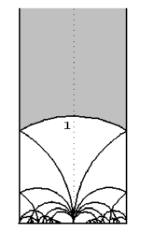
Figure 1: A possible fundamental domain (gray area) for the action of the $SL(2,\mathbb{Z})$ modular group on the upper half-plane. The upper-half plane parametrizes the possible values of $\tau$ (or $\rho$): the moduli of a two-torus. The gray domain can be folded into an $S^{2}$ with three special points (the two orbifold points: $\tau_{\mathbb{Z}_{6}}=e^{2\pi i/6}$ and $\tau_{\mathbb{Z}_{4}}=i$, and the decompactification point: $\tau\rightarrow i\infty$).

2.2 Two dimensions

In order to construct semi-flat fibrations in two dimensions, let us consider the dynamics first. Type IIA on a flat two-torus can be described by the effective action in Einstein frame

$$S=\int d^{8}x\sqrt{g}\left(R+\frac{\partial_{\mu}\tau\partial^{\mu}\bar{\tau}}{\tau_{2}^{2}}+\frac{\partial_{\mu}\rho\partial^{\mu}\bar{\rho}}{\rho_{2}^{2}}\right)$$ (2.1)

where $\tau$ is the complex structure of the torus, and $\rho=b+iV/2$ is the Kähler modulus as described earlier. The action is invariant under the $SL(2,\mathbb{Z})_{\tau}\times SL(2,\mathbb{Z})_{\rho}$ perturbative duality group, which acts on $\tau$ and $\rho$ by fractional linear transformations.

Variation with respect to $\tau$ gives

$$\partial\bar{\partial}\tau+\frac{2\partial\tau\bar{\partial}\tau}{\bar{\tau}-\tau}=0;$$ (2.2)

and $\rho$ obeys the same equation. Stringy cosmic string solutions to the EOM can be obtained by choosing a complex coordinate $z$ on two of the remaining eight dimensions, and taking $\tau(z)$ a holomorphic section of an $SL(2,\mathbb{Z})$ bundle. Such solutions are not modified by considering the following ansatz for the metric around the string

$$ds^{2}=ds_{\textrm{Mink}}^{2}+e^{\psi(z,\bar{z})}dzd\bar{z}+ds_{\textrm{fiber}}^{2}$$ (2.3)

where

$$ds_{\textrm{fiber}}^{2}=\frac{1}{\tau_{2}}\left(\begin{array}[]{cc}1&\tau_{1}\\ \tau_{1}&\ |\tau|^{2}\end{array}\right)$$ (2.4)

The Einstein equation is the Poisson equation,

$$\partial\bar{\partial}\psi=\partial\bar{\partial}\textrm{log}\,\tau_{2}$$ (2.5)

Far away from the strings, the metric of the base goes like [12]

$$ds^{2}_{2D}\sim|z^{-N/12}dz|^{2}$$ (2.6)

where $N$ is the number of strings. This can be coordinate transformed by $\tilde{z}=z^{1-N/12}$ to a flat metric with $2\pi N/12$ deficit angle.

Solutions and orbifold points. One could in principle write down solutions by means of the $j$-function,

$$j(\tau)=\eta(\tau)^{-24}(\theta^{8}_{1}(\tau)+\theta^{8}_{2}(\tau)+\theta^{8}_{3}(\tau))^{3}$$ (2.7)

which maps the $\tau_{\mathbb{Z}_{6}}=e^{2\pi i/6}$ and $\tau_{\mathbb{Z}_{4}}=i$ orbifold points to 0 and 1, respectively. The $\tau_{2}\rightarrow\infty$ degeneration point gets mapped to $j\rightarrow\infty$. A simple solution would then be

$$j(\tau)=\frac{1}{z-z_{0}}+j_{0}$$ (2.8)

At infinity, the shape of the fiber is constant, i.e. $\tau_{\infty}=j^{-1}(j_{0})$ and thus this non-compact solution may be glued to any other solution with constant $\tau$ at infinity. However, since $\tau$ covers the entire fundamental domain once, there will be two points in the base where $\tau(z)=\tau_{\mathbb{Z}_{6}}$ or $\tau_{\mathbb{Z}_{4}}$. Over these points, the fiber is an orbifold of the two-torus. These singular points cannot be resolved in a Ricci-flat way and we can’t use this solution for superstrings.

There is, however, a six-string solution which evades this problem [12]. It is possible to collect six strings together in a way that $\tau$ approaches a constant value at infinity. $\tau$ can be given implicitly by e.g.

$$y^{2}=x(x-1)(x-2)(x-z)$$ (2.9)

There are no orbifold points now because $\tau$ can be written as a holomorphic function over the base. The above equation describes three double degenerations, that is, three strings of tension twice the basic unit. In the limit when the strings are on top of one another, we obtain what is known (according to the Kodaira classification) as a $D_{4}$ singularity with deficit angle $180^{\circ}$.

The monodromy of the fiber around this singularity is described by

$$\mathcal{M}_{D_{4}}=\left(\begin{array}[]{rr}-1&0\\ 0&\ -1\end{array}\right)$$ (2.10)

acting on $\binom{\omega_{1}}{\omega_{2}}$with $\tau\equiv{\omega_{1}\over\omega_{2}}$. This monodromy decomposes into that of six elementary strings which are mutually non-local.

This can be generalized to more than six strings using the Weierstrass equation

$$y^{2}=x^{3}+f(z)x+g(z)$$ (2.11)

The modular parameter of the torus is determined by

$$j(\tau(z))=\frac{4f^{3}}{4f^{3}+27g^{2}}$$ (2.12)

Whenever the numerator vanishes, $\tau=\tau_{\mathbb{Z}_{6}}$ and we are at an orbifold point. We see however that it is a triple root of $f^{3}$ and no orbifolding of the fiber is necessary. The same applies for the $\mathbb{Z}_{4}$ points. The strings are located where $\tau_{2}\rightarrow\infty$ that is where the modular discriminant $\Delta\equiv 4f^{3}+27g^{2}$ vanishes. Note that the monodromy of the fibers around a smooth point is automatically the identity in such a construction.

Kodaira classification. Degenerations of elliptic fibrations have been classified according to their monodromy by Kodaira. For convenience, we summarize the result in the following table [21]:

ord(f)	ord(g)	ord($\Delta$)	monodromy	singularity
$\geq 0$	$\geq 0$	0	$\left(\begin{array}[]{cc}1&0\\ 0&1\end{array}\right)$	none
$0$	$0$	$n$	$\left(\begin{array}[]{cc}1&n\\ 0&1\end{array}\right)$	$A_{n-1}$
$\geq 1$	$1$	$2$	$\left(\begin{array}[]{cc}1&1\\ -1&0\end{array}\right)$	none
$1$	$\geq 2$	$3$	$\left(\begin{array}[]{cc}0&1\\ -1&0\end{array}\right)$	$A_{1}$
$\geq 2$	$2$	$4$	$\left(\begin{array}[]{cc}0&1\\ -1&-1\end{array}\right)$	$A_{2}$
$2$	$\geq 3$	$n+6$	$\left(\begin{array}[]{cc}-1&-n\\ 0&-1\end{array}\right)$	$D_{n+4}$
$\geq 2$	$3$	$n+6$	$\left(\begin{array}[]{cc}-1&-n\\ 0&-1\end{array}\right)$	$D_{n+4}$
$\geq 3$	$4$	$8$	$\left(\begin{array}[]{cc}-1&-1\\ 1&0\end{array}\right)$	$E_{6}$
$3$	$\geq 5$	$9$	$\left(\begin{array}[]{cc}0&-1\\ 1&0\end{array}\right)$	$E_{7}$
$\geq 4$	$5$	$10$	$\left(\begin{array}[]{cc}0&-1\\ 1&1\end{array}\right)$	$E_{8}$

Constructing K3. One can construct a compact example where the fiber experiences 24 $A_{0}$ degenerations. In the Weierstrass description (2.11), this means that $f$ has degree 8, $g$ has degree 12, and $\Delta$ has degree 24. This is the semi-flat description of a $K3$ manifold. In a certain limit where we group the strings into four composite $D_{4}$ singularities, the base is flat and the total space becomes $T^{4}/\mathbb{Z}_{2}$. The base can be obtained by gluing four flat triangles as seen in Figure 3. At each $D_{4}$ degeneration, the base has $180^{\circ}$ deficit angle which adds up to $4\pi$ and closes the space into a flat sphere with the curvature concentrated at four points.

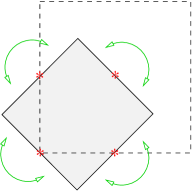
Figure 2: Base of the $T^{4}/\mathbb{Z}_{2}$ orbifold. The $\mathbb{Z}_{2}$ action inverts the base coordinates and has four fixed points denoted by red stars. They have $180^{\circ}$ deficit angle. As the arrows show, one has to fold the diagram and this gives an $S^{2}$.

As we have seen, in two dimensions the Weierstrass equation solves the problem of orbifold points. In higher dimensions, we don’t have this tool but we can still try to glue patches of spaces in order to get compact solutions. Gluing is especially easy if the base is flat. However, generically this is not the case. Having a look at the Einstein equation (2.2), we see that a flat base can be obtained if $\tau(z)$ is constant. This happens in the case of $D_{4}$ and $E_{n}$ singularities. Our discussion in this paper will (unfortunately) be restricted to these singularities.

The cosmic string metric is singular in the above semi-flat description. It must be slightly modified in order to get a smooth Calabi-Yau metric for the total space. This will be discussed in Appendix B.

Figure 3: Flat $S^{2}$ base constructed from four triangles: base of $K3$ in the $\mathbb{Z}_{2}$ orbifold limit.

2.3 Three dimensions

In two dimensions, the only smooth compact Calabi-Yau is the $K3$ surface. In three dimensions, there are many different spaces and therefore the situation is much more complicated. The SYZ conjecture [14] says that every Calabi-Yau threefold which has a geometric mirror, is a special Lagrangian $T^{3}$ fibration with possibly degenerate fibers at some points. For the generic case, the base is an $S^{3}$. Without the special Lagrangian condition, the conjecture has been well understood in the context of topological mirror symmetry [22, 23]. There, the degeneration loci form a (real) codimension two subset in the base. A graph $\Gamma$ is formed by edges and trivalent vertices. The fiber suffers from monodromy around the edges. This is specified by a homomorphism

$$M:\ \pi_{1}(S^{3}\setminus\Gamma)\longrightarrow SL(3,\mathbb{Z})$$ (2.13)

There are two types of vertices which contribute $\pm 1$ to the Euler character of the total space. At the vertices, the topological junction condition relates the monodromies of the edges.

One of the most studied non-trivial Calabi-Yau spaces is the quintic in $\mathbb{P}^{4}$. However, even the topological description of this example is fairly complicated [22]. The topological construction contains $250+50$ vertices and $450$ edges in the $S^{3}$ base.

Constructing not only topological, but special Lagrangian SYZ fibrations is a much harder task. In fact, it is expected that away from the semi-flat limit, the real codimension two singular loci in the base get promoted to codimension one singularities, i.e. surfaces in three dimensions. These were termed ribbon graphs [25] and their description remains elusive.

A compact orbifold example. In the following, we will describe the singular $T^{6}/\mathbb{Z}_{2}\times\mathbb{Z}_{2}$ orbifold in the SYZ fibration picture. One starts with $T^{6}$ that is a product of three tori with complex coordinates $z_{i}$. Without discrete torsion, the orbifold action is generated by the geometric transformations,

$$\alpha:(z_{1},z_{2},z_{3})\mapsto(-z_{1},-z_{2},z_{3})$$ (2.14)

$$\beta:(z_{1},z_{2},z_{3})\mapsto(-z_{1},z_{2},-z_{3})$$ (2.15)

These transformations have unit determinant and thus the resulting space may be resolved into a smooth Calabi-Yau manifold.

In order to obtain a fibration structure, we need to specify the base and the fibers. For the base coordinates, we choose $x_{i}\equiv\textrm{Re}(z_{i})$ and for the fibers $y_{i}\equiv\textrm{Im}(z_{i})$. Under the orbifold action, fibers are transformed into fibers and they don’t mix with the base.

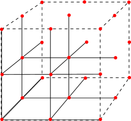
Figure 4: Singularities in the base of $T^{6}/\mathbb{Z}_{2}\times\mathbb{Z}_{2}$. The big dashed cube is the original $T^{3}$ base. The orbifold group generates the singular lines as depicted in the figure. The red dots show the intersection points of these edges.

Degeneration loci in the base. The base originally is a $T^{3}$. What happens after orbifolding? If we fix, for instance, the $x_{3}$ coordinate, then the orbifold action locally reduces to $\alpha$ (since the other two non-trivial group elements change $x_{3}$). This means that we simply obtain four fixed points in this slice of the base. This is exactly analogous to the $T^{4}/\mathbb{Z}_{2}$ example. The fixed points correspond to $D_{4}$ singularities with a deficit angle of $180^{\circ}$. As we change $x_{3}$, we obtain four parallel edges in the base. By keeping instead $x_{1}$ or $x_{2}$ fixed, we get perpendicular lines corresponding to conjugate $D_{4}$s whose monodromies act on another $T^{2}$ in the $T^{3}$ fiber. Altogether, we get $3\times 4$ lines of degeneration as depicted in Figure 4. These edges meet at (half-)integer points in the $T^{3}$ base.

Some parts of the base have been identified by the orbifold group. We can take this into account by a folding procedure which we have already seen for $T^{4}/\mathbb{Z}_{2}$. The degeneration loci are the edges of a cube. The volume of this cube is $\frac{1}{8}$ of the volume of the original $T^{3}$. The base can be obtained by gluing six pyramids on top of the faces (see Figure 5). The top vertices of these pyramids are the reflection of the center of the cube on the faces and thus the total volume is twice that of the cube. This polyhedron is a Catalan solid: the rhombic dodecahedron. (Note that one can also construct the same base by gluing two separate cubes together along their faces.)

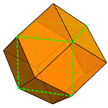
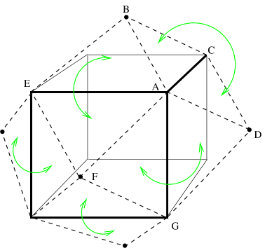
Figure 5: (i) Rhombic dodecahedron: fundamental domain for the base of $T^{6}/\mathbb{Z}_{2}\times\mathbb{Z}_{2}$. Six pyramids are glued on top of the faces of a cube. Neighboring pyramid triangles give rhombi since the vertices are coplanar (e.g. $ABCD$). (ii) The $S^{3}$ base can be constructed by identifying triangles as shown by the arrows. After gluing, the deficit angle around cube edges is $180^{\circ}$ which is appropriate for a $D_{4}$ singularity. The dihedral angles of the dashed lines are $120^{\circ}$ and since three of them are glued together, there is no deficit angle. The tips of the pyramids get identified and the space finally becomes an $S^{3}$.

In order to have a compact space, we finally glue the faces of the pyramids to neighboring faces (see the right-hand side of Figure 5). This is analogous to the case of $T^{4}/\mathbb{Z}_{2}$ where triangles were glued along their edges (Figure 2).

The topology of the base. The base is an $S^{3}$ which can be seen as follows. First fold the three rombi $ABCD$, $AFGD$ and $ABEF$, and the corresponding three on the other side of the fundamental domain. Then, we are still left with six rhombi that we need to fold. It is not hard to see that the problem is topologically the same as having a $B^{3}$ ball with boundary $S^{2}$. Twelve triangles cover the $S^{2}$ and we need to glue them together as depicted in Figure 6. This operation is the same as taking the $S^{2}$ and identifying its points by an $x\mapsto-x$ flip. This on the other hand, exhibits the space as an $S^{1}$ fibration over $D^{2}$. The fiber vanishes at the boundary of the disk. This is further equivalent to an $S^{2}$ fibration over an interval where the fiber vanishes at both endpoints. This space is simply an $S^{3}$. The degeneration loci are on the $S^{2}$ equator of this $S^{3}$ base and form the edges of the cube.

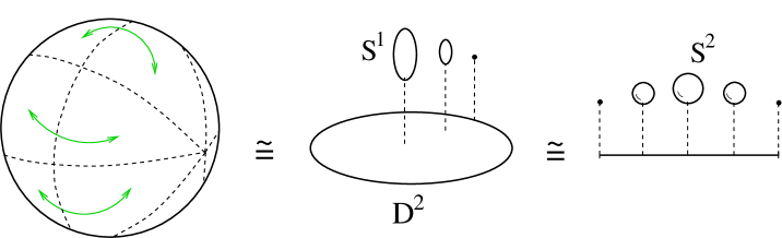
Figure 6: The base of $T^{6}/\mathbb{Z}_{2}\times\mathbb{Z}_{2}$ is homeomorphic to a three-ball with an $S^{2}$ boundary which has to be folded as shown in the figure.

Edges and vertices. The monodromies of the edges are shown in Figure 7. The letters on the degeneration edges denote the following $SL(3)$ monodromies:

$$x=\left(\begin{array}[]{rrr}1&0&0\\ 0&-1&0\\ 0&0&-1\end{array}\right)\quad y=\left(\begin{array}[]{rrr}-1&0&0\\ 0&\ 1&0\\ 0&0&-1\end{array}\right)\quad z=\left(\begin{array}[]{rrr}-1&0&0\\ 0&-1&0\\ 0&0&\ 1\end{array}\right)$$ (2.16)

Figure 7: Monodromies for the edges.

This orbifold example contained $D_{4}$ strings. These are composite edges made out of six “mutually non-local” elementary edges. The edges have $180^{\circ}$ deficit angle around them which is $6\times\frac{\pi}{6}$ where $\frac{\pi}{6}$ is the deficit angle of the elementary string.

Note that the base is flat. This made it possible to easily glue the fundamental cell to itself yielding a compact space. Since the edges around any vertex meet in a symmetric way, the cancellation of forces is automatic.

There are other spaces that one can describe using $D_{4}$ edges and the above mentioned composite vertices. Some examples are presented in Section 4. The strategy is to make a compact space by gluing polyhedra like the above described cubes, then make sure that the dihedral deficit angles are appropriate for the $D_{4}$ singularity.

2.4 Flat vertices

Codimension two degeneration loci meet at vertices in the base. In the generic case, these are trivalent vertices of elementary strings. Such strings have $30^{\circ}$ deficit angle around them measured at infinity. This creates a solid deficit angle around the vertex.

In some cases when composite singularities meet, the base is flat and the vertex is easier to understand. In particular, the total deficit angle arises already in the vicinity of the strings. An example was given in Section 2.3 where composite vertices arise from the “collision” of three $D_{4}$ singularities (see Figure 5). The singular edges have a deficit angle $\pi$. The vertex can be constructed by taking an octant of three dimensional space and gluing another octant to it along the boundary walls. The curvature is then concentrated in the axes. The solid angle can be computed as twice the solid angle of an octant. This gives $\pi$ (or a deficit solid angle of $3\pi$).

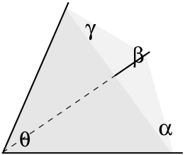
Figure 8: The solid angle at the apex is determined by the dihedral angles between the planes.

In the general (flat) case, a composite vertex may be described by gluing two identical cones (the analogs of octants). Such a cone is shown in Figure 8. Note that the solid angle spanned by three vectors is given by the formula

$$\theta=\alpha+\beta+\gamma-\pi$$ (2.17)

where $\alpha$, $\beta$ and $\gamma$ are the dihedral angles at the edges. This can be used to compute the solid angle around a composite vertex.

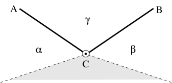
Figure 9: Flat vertex. $A$, $B$ and $C$ are singular edges. $C$ is pointing towards the reader. The dashed lines must be glued together to account for the deficit angle around $C$.

The singular edges have a tension which is proportional to the deficit angle around them. This leads to the problem of force balance. In Figure 9, a flat vertex is shown. The two solid lines ($A$ and $B$) are degeneration loci. The third edge ($C$) is pointing towards the reader as indicated by the arrow head. The deficit angle around $C$ is shown by the shaded area. In the weak tension limit (where we rescale the deficit angles by a small number), one condition for force balance is that these edges are in a plane. (Otherwise, energy could be decreased by moving the vertex.) This can be generalized for almost flat spaces by ensuring that $\alpha+\beta=\gamma$. This is automatic when we construct the neighborhood of a vertex by gluing two identical cones.

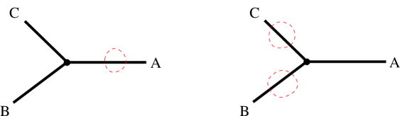
Figure 10: Junction condition for monodromies. The red loop around $A$ can be smoothly deformed into two loops around $B$ and $C$.

Another problem to be solved is related to the fiber monodromies. These can be described by matrices $A$, $B$ and $C$ (see Figure 10). The loop around one of the edges (say $A$) can be smoothly deformed into the union of the other two ($B,C$). This gives the monodromy condition $ABC=1$.

Some composite strings can be easier described than elementary ones because the base metric can be flat around them. Such singularities are $D_{4}$, $E_{6}$, $E_{7}$ and $E_{8}$ with deficit angles $\pi$, $4\pi/3$, $3\pi/2$ and $5\pi/3$, respectively [12]. Vertices where composite lines meet can also be easily found by studying flat $\mathbb{C}^{3}$ orbifolds. Here we list some of the vertices that will later arise in the examples.

orbifold group	colliding singularities	solid angle
$\mathbb{Z}_{2}\times\mathbb{Z}_{2}$	$D_{4}-D_{4}-D_{4}$	$\pi$
$\mathbb{Z}_{2}\times\mathbb{Z}_{4}$	$D_{4}-D_{4}-E_{7}$	$\pi/2$
$\Delta_{12}$	$D_{4}-E_{6}-E_{6}$	$\pi/3$
$\Delta_{24}$	$D_{4}-E_{6}-E_{7}$	$\pi/6$

Table 1: Examples for composite vertices.

We have already seen the $\mathbb{Z}_{2}\times\mathbb{Z}_{2}$ vertex in Section 2.3. If the vertex is located at the origin, then the strings are stretched along the coordinate axes,

$$D^{(1)}_{4}:(1,0,0)\qquad D^{(2)}_{4}:(0,1,0)\qquad D^{(3)}_{4}:(0,0,1)$$ (2.18)

The second example is generated by

$$\alpha:(z_{1},z_{2},z_{3}) \mapsto (-z_{3},z_{2},z_{1})$$

$$\beta:(z_{1},z_{2},z_{3}) \mapsto (z_{1},-z_{2},-z_{3})$$

It contains different colliding singularities. Their directions are given by

$$D^{(1)}_{4}:(1,0,0)\qquad D^{(2)}_{4}:(1,0,1)\qquad E_{7}:(0,1,0)$$ (2.19)

The $\Delta_{12}$ group has $(\mathbb{Z}_{2})^{2}$ and $\mathbb{Z}_{3}$ subgroups. It is generated by

$$\alpha:\,(z_{1},z_{2},z_{3}) \mapsto (z_{2},z_{3},z_{1})$$

$$\beta:\,(z_{1},z_{2},z_{3}) \mapsto (-z_{1},-z_{2},z_{3})$$

The strings directions are

$$D_{4}:(1,0,0)\qquad E^{(1)}_{6}:(1,1,1)\qquad E^{(2)}_{6}:(1,1,-1)$$ (2.20)

The last example is generated by combining $\mathbb{Z}_{3}$ and $\mathbb{Z}_{4}$ generators,

$$\alpha:(z_{1},z_{2},z_{3}) \mapsto (z_{2},z_{3},z_{1})$$

$$\beta:(z_{1},z_{2},z_{3}) \mapsto (-z_{2},z_{1},z_{3})$$

which generate the $\Delta_{24}$ group. The direction of the strings are the following,

$$D_{4}:(1,1,0)\qquad E_{6}:(1,1,1)\qquad E_{7}:(1,0,0)$$ (2.21)

This is not an exhaustive list; a thorough study based on the finite subgroups of $SU(3)$ [27] would be interesting.

3 Stringy monodromies

In this section, we wish to extend the discussion by including the full perturbative duality group of type II string theory on $T^{3}$ in the possible set of monodromies. We will find that this duality group can be interpreted as the geometric duality group of an auxiliary $T^{4}$. The extra circle is to be distinguished from the M-theory circle but it is related to it by a U-duality transformation.

For simplicity, the Ramond-Ramond field strengths will be turned off. This allows us to use perturbative dualities only. However, in moduli stabilization these fields play an important role. In fact, in the Appendices C and D, we use U-duality [28] monodromies which act on RR-fields in order to describe two familiar phenomena.

From the worldsheet point of view, string compactifications are expected to be typically non-geometric, since the 2d CFT does not necessarily have a geometric target space. Even though we construct our examples directly based on intuition from supergravity, they will have a worldsheet description as modular invariant asymmetric orbifolds.

For other related works on non-geometric spaces, see [29, 11, 30, 31, 32, 33, 34, 35, 36, 37, 38, 39, 40, 41, 7, 42, 43] and references therein.

In the following, we study the perturbative duality group in Type IIA string theory compactified on a flat three-torus. We gain intuition by studying the reduced 7d Lagrangian of the supergravity approximation. Finally we discuss how U-duality relates non-geometric compactifications to $G_{2}$ manifolds in M-theory which will be fruitful when constructing examples in the next section.

3.1 Reduction to seven dimensions

Action and symmetries. Let us consider the bosonic sector of (massless) 10d Type IIA supergravity,

$$S_{\textrm{IIA}}=S_{\textrm{NS}}+S_{\textrm{R}}+S_{\textrm{CS}}$$ (3.22)

where

$$S_{\textrm{NS}}=\frac{1}{2\kappa^{2}_{10}}\int d^{10}x\sqrt{-g}\,e^{-2\phi}(R+4\partial_{\mu}\phi\partial^{\mu}\phi-\frac{1}{2}|H_{3}|^{2})$$ (3.23)

$$S_{\textrm{R}}=-\frac{1}{4\kappa^{2}_{10}}\int d^{10}x\sqrt{-g}\,(|F_{2}|^{2}+|\tilde{F}_{4}|^{2})$$ (3.24)

and the Chern-Simons term is

$$S_{\textrm{CS}}=-\frac{1}{4\kappa^{2}_{10}}\int B\wedge F_{4}\wedge F_{4}$$ (3.25)

with $\tilde{F}_{4}=dA_{3}-A_{1}\wedge dB$ and $\kappa^{2}_{10}=\kappa^{2}_{11}/2\pi R$.

First we set the RR fields to zero. This truncates the theory to the NS part which is identical to the IIB $S_{\textrm{NS}}$ action. Compactifying Type IIA on a flat $T^{3}$ yields the perturbative T-duality group $SO(3,3,\mathbb{Z})$ which acts on the coset $SO(3,3,\mathbb{R})/SO(3)^{2}$.

The equivalences of Lie algebras

$$\mathfrak{so}(3,3)\cong\mathfrak{sl}(4)$$ (3.26)

$$\mathfrak{so}(3)\oplus\mathfrak{so}(3)\cong\mathfrak{su}(2)\oplus\mathfrak{su}(2)\cong\mathfrak{so}(4)$$ (3.27)

enable us to realize the T-duality group as an $SL(4,\mathbb{Z})$ action on $SL(4,\mathbb{R})/SO(4)$. This latter space is simply the moduli space of a flat $T^{4}$ with constant volume. Therefore, we can think of the T-duality group as the mapping class group of an auxiliary four-torus of unit volume. What is the metric on this $T^{4}$ in terms of the data of the $T^{3}$? To answer this question, we have to study the Lagrangian.

Reduction to seven dimensions. One obtains the following terms after reduction on $T^{3}$ [44] (see Appendix A for more details and notation)

$$S=\int dx\sqrt{-g}e^{-\phi}\mathcal{L}$$ (3.28)

with $\mathcal{L}=\mathcal{L}_{1}+\mathcal{L}_{2}+\mathcal{L}_{3}+\mathcal{L}_{4}$ and

$$\mathcal{L}_{1} = R+\partial_{\mu}\phi\partial^{\mu}\phi$$ (3.29)

$$\mathcal{L}_{2} = \frac{1}{4}(\partial_{\mu}G_{\alpha\beta}\partial^{\mu}G^{\alpha\beta}-G^{\alpha\beta}G^{\gamma\delta}\partial_{\mu}B_{\alpha\gamma}\partial^{\mu}B_{\beta\delta})$$ (3.30)

$$\mathcal{L}_{3} = -\frac{1}{4}g^{\mu\rho}g^{\nu\lambda}(G_{\alpha\beta}F^{(1)\alpha}_{\mu\nu}F^{(1)\beta}_{\rho\lambda}+G^{\alpha\beta}H_{\mu\nu\alpha}H_{\rho\lambda\beta})$$ (3.31)

$$\mathcal{L}_{4} = -\frac{1}{12}H_{\mu\nu\rho}H^{\mu\nu\rho}$$ (3.32)

The relation of these fields and the ten dimensional fields are presented in Appendix A. In order to see the $SO(d,d,\mathbb{Z})$ symmetry, one introduces the symmetric positive definite $2d\times 2d$ matrix

$$M=\left(\begin{array}[]{cc}G^{-1}&G^{-1}B\\ BG^{-1}&\ \ G-BG^{-1}B\end{array}\right)\in SO(3,3)$$ (3.33)

The kinetic terms $\mathcal{L}_{2}$ can be written as the $\sigma-$model Lagrangian

$$\mathcal{L}_{2}=\frac{1}{8}\textrm{Tr}(\partial_{\mu}M^{-1}\partial^{\mu}M)$$ (3.34)

The other terms in the Lagrangian are also invariant under $SO(3,3)$.

The SL(4) duality symmetry and “N-theory”. Let us now put the bosonic action in a manifestly $SL(4)$ invariant form (see [45]). Rewrite $\mathcal{L}_{2}$ as

$$\mathcal{L}_{2}=\frac{1}{8}\textrm{Tr}(\partial_{\mu}M^{-1}\partial^{\mu}M)=\frac{1}{4}\textrm{Tr}(\partial_{\mu}N^{-1}\partial^{\mu}N),$$ (3.35)

where we introduced the symmetric $SL(4)$ matrix

$$N_{4\times 4}=(\textrm{det}\,G)^{-1/2}\left(\begin{array}[]{cc}G&G\vec{b}\\ \vec{b}^{T}G&\ \ \textrm{det}\,G+\vec{b}^{T}G\vec{b}\end{array}\right)$$ (3.36)

$$B_{ij}=\epsilon_{ijk}b_{k}\qquad b_{i}=\frac{1}{2}\epsilon_{ijk}B_{jk}.$$ (3.37)

The equality of the Lagrangians can be checked by lengthy algebraic manipulations (or a computer algebra software). We included the Hodge-dualized B-field in the metric as a Kaluza-Klein vector. The inverse of $N$ is

$$N^{-1}=(\textrm{det}\,G)^{-1/2}\left(\begin{array}[]{cc}(\textrm{det}\,G)G^{-1}+\vec{b}^{T}b&\ \ -\vec{b}\\ -\vec{b}^{T}&\ \ 1\end{array}\right).$$ (3.38)

Keeping $N$ symmetric, the Lagrangian is invariant under the global transformation,

$$N(x)\mapsto U^{T}N(x)U,\ \ \textrm{with}\ U\in SL(4).$$ (3.39)

A useful device for interpreting $N$ is the following. Note that we would get the exact same bosonic terms of $\mathcal{L}_{1}$ and $\mathcal{L}_{2}$, if we were to reduce an eleven dimensional classical theory to seven dimensions. This theory is given by the Einstein-Hilbert action plus a scalar, the “11d dilaton”

$$S=\int d^{11}x\sqrt{-\tilde{g}}\,e^{-\phi}(R(\tilde{g})+\partial_{\mu}\phi\partial^{\mu}\phi)$$ (3.40)

This Lagrangian contains no B-field. The description in terms of (3.40) is only useful when $\mathcal{L}_{3}$ and $\mathcal{L}_{4}$ vanish. This means that $F^{(1)\alpha}_{\mu\nu}=H_{\mu\nu\alpha}=H_{\mu\nu\rho}=0$. Since the size of $T^{4}$ is constant, its dimensions are not treated on the same footing as the three geometric fiber dimensions. It is similar to the situation in F-theory [13], where the area of the $T^{2}$ is fixed and the Kähler modulus of the torus is not a dynamical parameter.

We have seen that the matrix $N$ can be interpreted as a semi-flat metric on a $T^{4}$ torus fiber. Part of this torus is the original $T^{3}$ fiber and the overall volume is set to one. The T-duality group $SO(3,3,\mathbb{Z})$ acts on $T^{4}$ in a geometric way. This means that we can hope to study non-geometric compactifications by studying purely geometric ones in higher dimension.

3.2 The perturbative duality group

In the previous section, we have transformed the coset space $SO(3,3)/SO(3)^{2}$ into $SL(4)/SO(4)$ via Eq. (3.36). We also would like to see how the discrete T-duality group $SO(3,3,\mathbb{Z})$ maps to $SL(4,\mathbb{Z})$. We will denote the $SO(3,3)$ matrices by $\mathcal{Q}$, and the $SL(4)$ matrices by $\mathcal{W}$.

SO(3,3)	SL(4)	dim	examples
spinor	fundamental	4	RR fields
fundamental	antisym. tensor	6	momenta & winding

Table 2: The two basic representations of the duality group.

Generators of SO(3,3,Z). It was shown in [46] that the following $SO(3,3,\mathbb{Z})$ elements generate the whole group

$$\mathcal{Q}_{1}(n)=\left(\begin{array}[]{c|c}\mathbbm{1}_{3\times 3}&n\\ \hline\cr 0&\ \mathbbm{1}_{3\times 3}\end{array}\right)\qquad\mathcal{Q}_{2}(R)=\left(\begin{array}[]{c|c}R&0\\ \hline\cr 0&\ (R^{-1})^{T}\end{array}\right)\qquad\mathcal{Q}_{3}=\left(\begin{array}[]{ccc|ccc}0&&&\ 1&&\\ &0&&&1&\\ &&1&&&0\\ \hline\cr 1&&&\ 0&&\\ &1&&&0&\\ &&0&&&1\end{array}\right)$$ (3.41)

where $n^{T}=-n$, $\textrm{det}\,R=\pm 1$. The first two matrices correspond to a change of basis of the compactification lattice. The last matrix is T-duality along the $x^{7}-x^{8}$ coordinates. Instead of using $\mathcal{Q}_{3}$ directly, we combine double T-duality with a $90^{\circ}$ rotation. This gives the $SO(3,3)$ matrix

$$\mathcal{\widetilde{Q}}_{3}=\left(\begin{array}[]{ccc|ccc}&&&&-1&\\ &&&\ 1&&\\ &&1&&&\\ \hline\cr&1&&&&\\ -1&&&&&\\ &&&&&1\end{array}\right)$$ (3.42)

Generators of SL(4,Z). In the Appendix of [47], it was shown that the above matrices have an integral $4\times 4$ spinor representation and in fact generate the entire $SL(4,\mathbb{Z})$. We now list the spinor representations corresponding to these generators.

• $\mathcal{Q}_{1}(n)$ is mapped to matrices

  $$\mathcal{W}_{1}(n)=\left(\begin{array}[]{rr|rc}1&&&\ n_{23}\\ &1&&\ n_{31}\\ \hline\cr&&\ 1&\ n_{12}\\ &&&1\end{array}\right)$$ (3.43)

  These are the generators corresponding to “T” transformations of various $SL(2)$ subgroups.

• $\mathcal{\widetilde{Q}}_{3}$ is mapped to

  $$\mathcal{\widetilde{W}}_{3}=\left(\begin{array}[]{rr|rr}1&&&\\ &1&&\\ \hline\cr&&&-1\\ &&\ 1&\end{array}\right)$$ (3.44)

  This corresponds to a modular “S” transformation. Note that $(\mathcal{\widetilde{W}}_{3})^{2}\neq\mathbbm{1}$.

• When $\textrm{det}\,R=+1$, the matrix $\mathcal{Q}_{2}(R)$ is mapped to the $SL(4,\mathbb{Z})$ matrix

  $$\mathcal{W}_{2}(R)=\left(\begin{array}[]{cc}R&0\\ 0&1\end{array}\right)$$ (3.45)

  For symmetric $R$ matrices it coincides with the prescription of Eq. (3.36).

• The $\textrm{det}\,R=-1$ case is more subtle. Even though Type IIA string theory is parity invariant, in the microscopic description reflecting an odd number of coordinates does not give a symmetry by itself. Since this transformation flips the spinor representations $16\leftrightarrow 16^{\prime}$, it must be accompanied by an internal symmetry $\Omega$ which changes the orientation of the world-sheet and thus exchanges the left-moving and right-moving spinors.

  $SO(3,3)$ has maximal subgroup $S(O(3)\times O(3))$ and hence has two connected components [32]. Inversion of an odd number of coordinates is not in the identity component. $SL(4,\mathbb{Z})$ is the double cover of the connected component of $SO(3,3,\mathbb{Z})$ only. We must allow for $\textrm{det}\,\mathcal{W}=\pm 1$ to obtain $Spin(3,3,\mathbb{Z})$, the double cover of the full $SO(3,3,\mathbb{Z})$. Then, the reflections of the $x^{7}$, $x^{8}$ or $x^{9}$ coordinates have the following representations

  $$\mathcal{W}_{I_{7}}=\textrm{diag}(-1,1,1,1)\qquad\mathcal{W}_{I_{8}}=\textrm{diag}(1,-1,1,1)\qquad\mathcal{W}_{I_{9}}=\textrm{diag}(1,1,-1,1)$$ (3.46)

  Upon restriction to $GL(3)\subset SO(3,3)$, the $Spin(3,3)$ group is a trivial covering.

  Ramond-Ramond fields transform in the spinor representation of the T-duality group. Therefore they form fundamental $SL(4)$ multiplets, for instance $(C_{7},C_{8},C_{9},C_{789})$. We can check the above representation for the coordinate reflections. Reflection of say $x^{7}$ combined with a flip of the three-form field gives

  $$(C_{7},C_{8},C_{9},C_{789})\mapsto(-C_{7},C_{8},C_{9},C_{789})$$ (3.47)

  which is precisely the action of $\mathcal{W}_{I_{7}}$.

3.3 Embedding $SL(2)^{2}$ in $SL(4)$

In order to get some intuition for the $SL(4)$ duality group that we discussed in the previous section, we first look at the simpler case of $T^{2}$ compactifications. In this section we describe how the T-duality group of $T^{2}$ compactifications can be embedded into the bigger $SL(4)$ group.

In eight dimensions, the duality group is $SL(2)_{\tau}\times SL(2)_{\rho}$ with the first factor acting on the $\tau$ complex structure of the torus and the second factor acting on $\rho=b+iV/2$ where $b=\int_{T^{2}}B$ and $V$ is the volume of $T^{2}$. If we consider a two dimensional base with complex coordinate $z$, then the equations of motion are satisfied if $\tau(z)$ and $\rho(z)$ are holomorphic sections of $SL(2,\mathbb{Z})$ bundles. Monodromies of $\tau$ around branch points points describe the geometric degenerations of the fibration. Monodromies of $\rho$, however, correspond to T-dualities and to the semi-flat description of NS5-branes. In particular, if there is a monodromy $\rho\mapsto\rho+1$ around a degeneration point in the base, then it implies $b\mapsto b+1$ which describes a unit magnetic charge for the B-field, i.e. an NS5-brane. The $\rho\mapsto-1/\rho$ monodromy on the other hand is a double T-duality along the $T^{2}$ combined with a $90^{\circ}$ rotation.

Let us denote the two-torus coordinates by $x^{7,8}$. In order to embed this $SL(2)\times SL(2)$ duality group into the $SL(4)$ of $T^{3}$ compactifications, we need to further compactify on a “spectator” circle of size $L$. We denote its coordinate by $x^{9}$. The metric on $T^{3}$ ($x^{9}-x^{10}-x^{11}$) is now

$$G_{3\times 3}=\left(\begin{array}[]{cc|c}g_{11}&g_{12}&\\ g_{21}&g_{22}&\\ \hline\cr&&\ L^{2}\end{array}\right)$$ (3.48)

Then, one can construct the $4\times 4$ metric on $T^{4}$ by the prescription of (3.36) which gives

$$N=(\textrm{det}\,g)^{-1/2}\left(\begin{array}[]{c|cc}\frac{1}{L}g_{2\times 2}&&\\ \hline\cr&\ L&Lb\\ &\ Lb&L(\textrm{det}\,g+b^{2})\\ \end{array}\right)\equiv\left(\begin{array}[]{cc}\frac{1}{L}\mathcal{T}_{2\times 2}&\\ &L\mathcal{R}_{2\times 2}\end{array}\right)$$ (3.49)

with

$$\mathcal{T}=\frac{1}{\tau_{2}}\left(\begin{array}[]{cc}1&\tau_{1}\\ \tau_{1}&|\tau|^{2}\end{array}\right)\qquad\mathcal{R}=\frac{1}{\rho_{2}}\left(\begin{array}[]{cc}1&\rho_{1}\\ \rho_{1}&|\rho|^{2}\end{array}\right)$$ (3.50)

The $\sigma$-model Lagrangian

$$\textrm{Tr}(\partial_{\mu}N^{-1}\partial^{\mu}N)=-2\left(\frac{\partial_{\mu}\tau\partial^{\mu}\bar{\tau}}{\tau_{2}^{2}}+\frac{\partial_{\mu}\rho\partial^{\mu}\bar{\rho}}{\rho_{2}^{2}}\right)$$ (3.51)

indeed gives the familiar kinetic terms for the torus moduli (in seven dimensions).

We have seen how the metric and the B-field parametrize the relevant subset of the $SL(4,\mathbb{R})/SO(4)$ coset space. The generators of the $SL(2,\mathbb{Z})\times SL(2,\mathbb{Z})$ duality group are also mapped to elements in $SL(4,\mathbb{Z})$. We now verify that these images in fact give the transformations that we expect.

• Geometric transformations

  These are simply generated by

  $$T=\left(\begin{array}[]{cc}1&1\\ 0&1\end{array}\right)\oplus\mathbbm{1}_{2\times 2}\quad\textrm{and}\quad S=\left(\begin{array}[]{cc}0&-1\\ 1&0\end{array}\right)\oplus\mathbbm{1}_{2\times 2}$$ (3.52)

  They act on $g_{2\times 2}$ by conjugation with the non-trivial $SL(2)$ part as expected. The determinant of $g$ stays the same. The first one is a Dehn-twist and the second one is a $90^{\circ}$ rotation.

• Non-geometric transformations

  The generators

  $$T^{\prime}=\mathbbm{1}_{2\times 2}\oplus\left(\begin{array}[]{cc}1&1\\ 0&1\end{array}\right)\quad\textrm{and}\quad S^{\prime}=\mathbbm{1}_{2\times 2}\oplus\left(\begin{array}[]{cc}0&-1\\ 1&0\end{array}\right)$$ (3.53)

  correspond respectively to the shift of the B-field and to a double T-duality on $x^{7,8}$ combined with a $90^{\circ}$ rotation. The latter one has the $SL(4)$ monodromy

  $$M=\left(\begin{array}[]{rr|rr}1&\ 0&\ 0&0\\ 0&1&0&0\\ \hline\cr 0&0&0&-1\\ 0&0&1&0\end{array}\right)$$ (3.54)

  This is basically an exchange of the $x^{9}-x^{10}$ coordinates and it transforms the $\mathcal{R}_{2\times 2}$ submatrix of $N$ into its inverse

  $$\mathcal{R}^{-1}=(\textrm{det}\,g)^{-1/2}\left(\begin{array}[]{cc}\textrm{det}\,g+b^{2}&-b\\ -b&1\end{array}\right)$$ (3.55)

  After this double T-duality, the (geometric) metric on $T^{3}$ becomes

  $$G_{3\times 3}\mapsto\widetilde{G}_{3\times 3}=\left(\begin{array}[]{c|r}\frac{1}{\textrm{det}g+b^{2}}\ g_{2\times 2}&0\\ \hline\cr 0&\ L^{2}\end{array}\right)$$ (3.56)

  The B-field transforms as

  $$b\mapsto\tilde{b}=-\frac{b}{\textrm{det}\,g+b^{2}}$$ (3.57)

  The metric $g$ on $T^{2}$ changes, in particular if $b=0$, then the volume gets inverted. Since we exchanged the $x^{9}-x^{10}$ coordinates, one might have expected that this affects the metric on $x^{9}$. However, we see that it remains the same as it should since it was only a spectator circle.

• Left-moving spacetime fermion number: $(-1)^{F_{L}}$

  This is a global transformation which inverts the sign of the Ramond-Ramond fields. It acts trivially on the vector representation of $SO(3,3)$ (which is the antisymmetric tensor of $SL(4)$). It will be important since T-duality squares to $(-1)^{F_{L}}$. In [11], its representation was determined,

  $$\mathcal{M}_{(-1)^{F_{L}}}=\left(\begin{array}[]{cc}-1&0\\ 0&-1\end{array}\right)\oplus\left(\begin{array}[]{cc}-1&0\\ 0&-1\end{array}\right)\in SL(2)\times SL(2)$$ (3.58)

  that is a $D_{4}$ monodromy combined with a $D^{\prime}_{4}$ (i.e. a conjugate $D_{4}$). This statement can be proven as follows. Let us define complex coordinates

  $$z_{L}=x^{7}_{L}+ix^{8}_{L}$$ (3.59)

  $$z_{R}=x^{7}_{R}+ix^{8}_{R}$$ (3.60)

  where $x_{L}$ and $x_{R}$ are the left- and right-moving components of the bosonic coordinates. We denote a transformation

  $$(z_{L},z_{R})\mapsto(e^{\theta_{L}}z_{L},\ e^{\theta_{R}}z_{R})$$ (3.61)

  by $\theta=(\theta_{L},\theta_{R})$. Then,

  $$\theta_{D_{4}}=(-\pi,-\pi)$$ (3.62)

  as it is a reflection of the bosonic coordinates. Moreover, we can use $D^{\prime}_{4}=S^{2}$ where $S$ is a double T-duality with a $90^{\circ}$ rotation. We have

  $$\theta_{S}=\underbrace{(-\pi,0)}_{\textrm{double T-duality}}+\underbrace{(\frac{\pi}{2},\frac{\pi}{2})}_{\textrm{$90^{\circ}$ rotation}}=(-\frac{\pi}{2},\frac{\pi}{2})$$ (3.63)

  from which we obtain

  $$\theta_{D^{\prime}_{4}}=2\times\theta_{S}=(-\pi,\pi)$$ (3.64)

  Finally,

  $$\theta_{D_{4}+D^{\prime}_{4}}=\theta_{D_{4}}+\theta_{D^{\prime}_{4}}=(-2\pi,0)$$ (3.65)

  which acts trivially on the bosons. However, it inverts the sign of the spinors from left movers which is precisely the action of $(-1)^{F_{L}}$. Finally, it can be embedded into $SL(4)$ simply as

  $$\mathcal{M}_{(-1)^{F_{L}}}=\textrm{diag}(-1,-1,-1,-1)$$ (3.66)

3.4 U-duality and $G_{2}$ manifolds

We have seen that upon compactifying Type IIA on $T^{3}$, a $T^{4}$ torus emerges. We will be eventually interested in compactifications to four dimensions. For vacua without fluxes and T-dualities, the total space of the $T^{3}$ fibration is a Calabi-Yau threefold. What can we say about the total space of the $T^{4}$ fibration?

Note that there is an analogous (more general) story in M-theory. Reducing eleven dimensional supergravity on a flat $T^{4}$ yields a Lagrangian that is symmetric under the $SL(5,\mathbb{R})$ U-duality group [28, 48, 49, 50]. By Hodge-dualizing the three-form $A_{IJK}=:\epsilon_{IJKL}X^{L}$ ($I,J,K,L=7,8,9,11$), one can define a $5\times 5$ matrix

$$G^{-1}=\left(\begin{array}[]{c|c}\omega g^{IJ}+\frac{1}{\omega}X^{I}X^{J}&\ -\frac{1}{\omega}X^{I}\\ \hline\cr-\frac{1}{\omega}X^{I}&\frac{1}{\omega}\end{array}\right)$$ (3.67)

which contains the geometric metric $g$ on $T^{4}$ as well. We denote the dimensions by $x^{7}$, $x^{8}$, $x^{9}$, $x^{11}$, $x^{10}$, respectively. The bosonic kinetic terms can be written as a manifestly $SL(5)$ invariant $\sigma$-model in terms of this metric [50].

We can embed the $4\times 4$ unit determinant matrix $N^{-1}$ (see Eq. 3.38) into the $5\times 5$ unit-determinant matrix $G^{-1}$ as follows

$$G^{-1}=\left(\begin{array}[]{cc|c}\delta g^{ij}+\frac{1}{\delta}b^{i}b^{j}&\ 0&-\frac{1}{\delta}b^{i}\\ 0&1&0\\ \hline\cr-\frac{1}{\delta}b^{i}&0&\frac{1}{\delta}\end{array}\right)$$ (3.68)

with $\delta\equiv(\textrm{det}\ g_{ij})^{1/2}$. By setting $\omega:=\delta$, we arrive at the previous form of the metric. If we now perform a U-duality corresponding to the $x^{10}-x^{11}$ flip, then the solution is transformed into pure geometry in the 11d picture,

$$G^{-1}=\left(\begin{array}[]{cc|c}\delta g^{ij}+\frac{1}{\delta}b^{i}b^{j}&\ -\frac{1}{\delta}b^{i}&\\ -\frac{1}{\delta}b^{i}&\frac{1}{\delta}&\\ \hline\cr&&\ 1\end{array}\right)\equiv\left(\begin{array}[]{c|c}g^{IJ}_{\textrm{new}}&\\ \hline\cr&\ 1\end{array}\right)$$ (3.69)

In 10d Type IIA language, this flip roughly corresponds to the exchange of the Ramond-Ramond one-form and the Hodge-dual of the B-field in the fiber directions.

In order to preserve minimal supersymmetry in four dimensions, one compactifies M-theory on a $G_{2}$ manifold. Semi-flat limits of $G_{2}$ manifolds are expected to exist by an SYZ-like argument [51]. Then, by the above U-duality in seven dimensions, a solution is obtained which is non-geometric from a 10d point of view as shown in this diagram

“Oxidation” seems obscure in this context since we only have the 7d spacetime equations of motion. However, for the special case of $D_{4}$ singularities, we will be able to “lift the solutions” to 10d: they turn out to be asymmetric orbifolds, similar to some examples in [11].

4 Compactifications with ${\bf D_{4}}$ singularities

In the previous sections, we studied the semi-flat limit of various geometries which had a fibration structure. This corner of the moduli space is a natural playground for T-duality since isometries appear along the fiber directions. Almost everywhere the space locally looks like $\mathbb{R}^{n}\times T^{n}$ and the duality group can simply be studied by a torus reduction of the supergravity Lagrangian. The idea is then to glue patches of the base manifold by also including the T-duality group in the transition functions. Since the duality group is discrete, such deformations are “topological” and a priori cannot be achieved continuously. From the 10d point of view, the total space becomes non-geometric in general. In seven dimensions, the $SO(3,3,\mathbb{Z})$ group can be realized as the mapping class group of a $T^{4}$ of unit volume. This geometrizes the non-geometric space by going one real dimension higher. Considering such compactifications to four dimensions which preserve ${\mathcal{N}}=1$ supersymmetry, U-duality suggests that the total space of the geometrized internal non-geometric space is a $G_{2}$ manifold.

In this section, we use these ideas to build non-geometric compactifications. We deform geometric orbifold spaces by hand and also study particular examples of $G_{2}$ manifolds. These examples will only contain (conjugate) $D_{4}$ singularities. This allows for a constant arbitrary shape for the fiber and the base is also locally flat. Even though the examples are singular and supergravity breaks down at the orbifold points, we can embed the solutions into Type IIA string theory where they give consistent non-geometric vacua realized as modular invariant asymmetric orbifolds.

4.1 Modified $K3\times T^{2}$

Let us first consider $K3$. The base of an elliptic fibration of $K3$ is an $S^{2}$. At the $T^{4}/\mathbb{Z}_{2}$ orbifold point, there are four $D_{4}$ singularities in the base (see Figure 3). The purely geometric $D_{4}$ monodromies are

$$\mathcal{M}_{D_{4}}=(\mathbbm{-1}_{2\times 2})\oplus\mathbbm{1}_{2\times 2}\ \in\ SL(2)_{\tau}\times SL(2)_{\rho}$$ (4.70)

By changing the monodromies by hand, it is possible to construct non-geometric spaces. In [11], $K3$ was modified into the union of two half K3’s which we denote by $\widetilde{K3}$. This non-geometric space has two ordinary $D_{4}$’s and two non-geometric $D^{\prime}_{4}$ singularities with monodromies

$$\mathcal{M}_{D^{\prime}_{4}}=\mathbbm{1}\oplus(\mathbbm{-1})$$ (4.71)

If we had changed one or three $D_{4}$s into $D^{\prime}_{4}$, then the monodromy at infinity would not be trivial. In fact, it would be $\mathcal{M}_{D_{4}}\cdot\mathcal{M}_{D^{\prime}_{4}}=\mathcal{M}_{(-1)^{F_{L}}}$. This means that the $T^{2}\times T^{2}$ fiber is orbifolded everywhere in the base by the $\mathbb{Z}_{2}$ action which inverts the fiber coordinates. In principle, this could be interpreted as an overall orbifolding by $(-1)^{F_{L}}$ which moves us from Type IIA to IIB. However, it is not clear what should happen to the odd number of $D_{4}$ and $D^{\prime}_{4}$ singularities as they don’t have a trivial monodromy at infinity in IIB either. Therefore, we do not consider such examples any further.

Let us now compactify further and consider $K3\times T^{2}$ or $\widetilde{K3}\times T^{2}$. The base is $S^{2}\times S^{1}$ where the second factor is the base of the two-torus as described in Section 2.1. The relevant monodromies are embedded in the $SL(4)$ duality group as follows

$$\mathcal{M}_{D_{4}}=\textrm{diag}(-1,-1,1,1)\qquad\mathcal{M}_{D^{\prime}_{4}}=\textrm{diag}(1,1,-1,-1)$$ (4.72)

Since in lower dimension the duality group is larger, one can consider another $D_{4}$-like monodromy

$$\mathcal{M}_{D^{\prime\prime}_{4}}=\textrm{diag}(1,-1,-1,1)$$ (4.73)

which is not in the $SL(2)\times SL(2)$ subgroup of $SL(4)$, and thus it was not possible for the case of $T^{2}$ compactifications. In principle, we can have spaces with monodromies

$$(2\times D_{4})+(2\times D^{\prime\prime}_{4})\quad\textrm{or}\quad(2\times D^{\prime}_{4})+(2\times D^{\prime\prime}_{4})$$ (4.74)

These are T-dual to each other by an $x^{7}-x^{10}$ flip. Thus, it is enough to consider the first one which is geometric since the monodromies act only in the upper-left $SL(3)$ subsector of $SL(4)$. However, this space is not Calabi-Yau. Supersymmetry suggests that in the base, parallel lines of singularities should have the same monodromies (possibly up to a factor of $(-1)^{F_{L}}$ as in the case of $\widetilde{K3}\times T^{2}$). This is not the case for this space. A way to explicitly see the absence of supersymmetry is to exhibit the total space as the $(\mathbb{R}\times T^{5})/\langle\alpha,\beta\rangle$ orbifold,

$$\alpha: (x,\theta_{1},\theta_{2}\,|\,\theta_{3},\theta_{4},\theta_{5})\mapsto(L-x,\theta_{1},-\theta_{2}\,|\,{-\theta_{3}},-\theta_{4},\theta_{5})$$ (4.75)

$$\beta: (x,\theta_{1},\theta_{2}\,|\,\theta_{3},\theta_{4},\theta_{5})\mapsto(-x,\theta_{1},-\theta_{2}\,|\,\theta_{3},-\theta_{4},-\theta_{5})$$ (4.76)

Here $x$, $\theta_{1,2}$ are coordinates on the base and $\theta_{3,4,5}$ are coordinates on the fiber. $x$ is non-compact and $\theta_{i}$ are periodic. The orbifold group $\langle\alpha,\beta\rangle$ also contains the element

$$\alpha\beta:\ (x,\theta_{1},\theta_{2}\,|\,\theta_{3},\theta_{4},\theta_{5})\mapsto(x+L,\theta_{1},\theta_{2}\,|\,{-\theta_{3}},\theta_{4},-\theta_{5})$$ (4.77)

which breaks supersymmetry because it projects out the gravitini.

We see that by considering conjugate $D_{4}$ singularities, in the above reducible case we do not obtain any other supersymmetric examples than those already considered in [11] even if the duality group is extended. Hence, we move on to threefolds in the next section.

4.2 Non-geometric $T^{6}/\mathbb{Z}_{2}\times\mathbb{Z}_{2}$

Let us consider the orbifold $T^{6}/\mathbb{Z}_{2}\times\mathbb{Z}_{2}$ that we described in detail in Section 2.3. Figure 7 shows the monodromies of the singular edges. These monodromies have the following $SL(4)$ representations,

$$x=\textrm{diag}(1,-1,-1,1)\quad y=\textrm{diag}(-1,1,-1,1)\quad z=\textrm{diag}(-1,-1,1,1)$$ (4.78)

These are of course geometric since they only act on the first three coordinates. How can we deform the orbifold into something non-geometric? There are three more $D_{4}$ type singularities that we can use. They have the following monodromies,

$$\bar{x}\equiv-x\qquad\bar{y}\equiv-y\qquad\bar{z}\equiv-z$$ (4.79)

These all invert the $x^{10}$ coordinate. A simple modification of $T^{6}/\mathbb{Z}_{2}\times\mathbb{Z}_{2}$ is possible by replacing the original monodromies by $\bar{x},\bar{y}$ or $\bar{z}$. The junction condition says that an even number of negative signs should meet at each vertex. Therefore, consistent monodromy assignments are given by switching signs along loops. There are five theories obtained this way as shown in Figure 11. Since these simple spaces have a geometric total space at this orbifold point of their moduli space, we call them “almost non-geometric”.

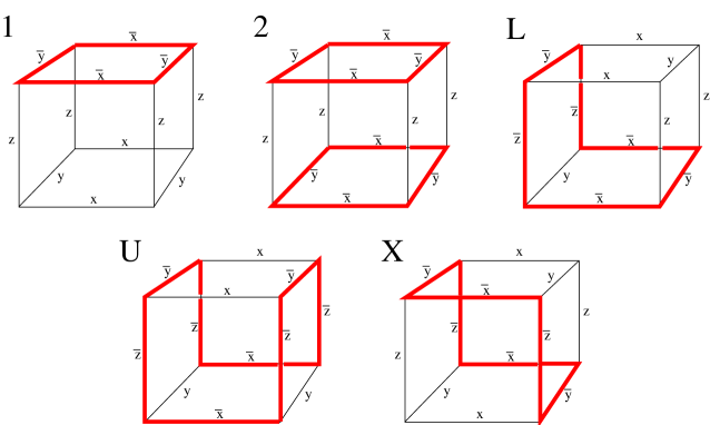
Figure 11: Almost non-geometric $T^{6}/\mathbb{Z}_{2}\times\mathbb{Z}_{2}$ spaces. Monodromies are modified along the red loops. We refer to the models as one-plaquette, two-plaquette, “L”, “U” and “X”, respectively.

4.3 Asymmetric orbifolds

In the previous section, we changed the monodromies by hand and obtained “almost non-geometric” spaces. In particular, monodromies in the loops contained the extra action of $(-1)^{F_{L}}$, which reverses the signs of all RR-charges,

$$x\cdot\mathcal{M}_{(-1)^{F_{L}}}=\bar{x}\qquad y\cdot\mathcal{M}_{(-1)^{F_{L}}}=\bar{y}\qquad z\cdot\mathcal{M}_{(-1)^{F_{L}}}=\bar{z}$$ (4.80)

where

$$\mathcal{M}_{(-1)^{F_{L}}}=\textrm{diag}(-1,-1,-1,-1)$$ (4.81)

Hence, we can realize the non-geometric spaces of the previous section as asymmetric orbifolds [52, 53] (see also [54, 55, 56, 57, 58, 59]). We consider the simple example of Figure 12: the one-plaquette model.

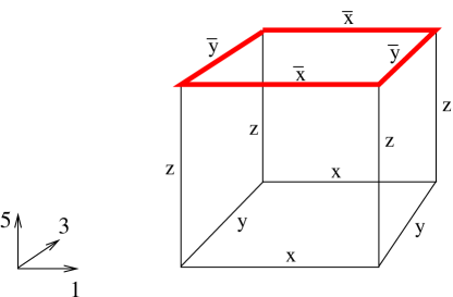
Figure 12: Simple non-geometric $T^{6}/\mathbb{Z}_{2}\times\mathbb{Z}_{2}$.

If we parametrize the $T^{6}$ torus by angles $\theta_{i}$, then the original $\mathbb{Z}_{2}\times\mathbb{Z}_{2}$ orbifold group action is generated by

$$\alpha:(\theta_{1},\theta_{2},\theta_{3},\theta_{4},\theta_{5},\theta_{6})\mapsto(-\theta_{1},-\theta_{2},-\theta_{3},-\theta_{4},\theta_{5},\theta_{6})$$ (4.82)

$$\beta:(\theta_{1},\theta_{2},\theta_{3},\theta_{4},\theta_{5},\theta_{6})\mapsto(-\theta_{1},-\theta_{2},\theta_{3},\theta_{4},-\theta_{5},-\theta_{6})$$ (4.83)

The base coordinates can be chosen to be $(\theta_{1},\theta_{3},\theta_{5})$. The singular edges along these directions have monodromies $(x,y,z)$, respectively.

Now the example of Figure 12 has modified monodromies. In particular, edges on the top of the cube have monodromies which include $(-1)^{F_{L}}$. We use the same trick as in Section 4.1: let us choose the vertical $x_{5}$ coordinate to be non-compact and then compactify it with an asymmetric action,

$$\alpha: \ (\theta_{1},\theta_{2},\theta_{3},\theta_{4},x_{5},\theta_{6})\mapsto(-\theta_{1},-\theta_{2},-\theta_{3},-\theta_{4},x_{5},\theta_{6})$$ (4.84)

$$\beta_{1}: \ (\theta_{1},\theta_{2},\theta_{3},\theta_{4},x_{5},\theta_{6})\mapsto(-\theta_{1},-\theta_{2},\theta_{3},\theta_{4},-x_{5},-\theta_{6})$$ (4.85)

$$\beta_{2}: \ (\theta_{1},\theta_{2},\theta_{3},\theta_{4},x_{5},\theta_{6})\mapsto(-\theta_{1},-\theta_{2},\theta_{3},\theta_{4},L-x_{5},-\theta_{6})\ \times\ (-1)^{F_{L}}$$ (4.86)

This realizes the example as an asymmetric orbifold. The Type IIA spectrum is computed in Appendix G. It has $\mathcal{N}=1$ supersymmetry with a gravity multiplet, 16 vector multiplets and 71 chiral multiplets.

The theory is consistent since decorating $D_{4}$ singularities with $(-1)^{F_{L}}$ does not destroy modular invariance. In the Green-Schwarz formalism, adding $(-1)^{F_{L}}$ changes the boundary conditions for the four complex left-moving fermionic coordinates as

$$D_{4}:(++--)\quad\longrightarrow\quad D_{4}\times(-1)^{F_{L}}:(--++)$$ (4.87)

Hence, the energy of the twisted sector ground state does not change and thus level-matching is satisfied [60]. In the RNS formalism, $(-1)^{F_{L}}$ does not act on the world-sheet fields and therefore the moding does not change. However, the left-moving GSO projection changes and various generalized discrete torsion signs show up in the twisted sectors as discussed in the Appendices. (See also related literature [58, 61].) For Abelian orbifolds, one-loop modular invariance implies higher loop modular invariance [60]. Here we are actually considering a non-Abelian orbifold for which level-matching is not sufficient for consistency. Further constraints may arise if a modular transformation takes a pair of commuting group elements $(g,h)$ into their own conjugacy class [62],

$$(g,h)\longrightarrow(g^{a}h^{b},g^{c}h^{d})=(pgp^{-1},php^{-1})$$ (4.88)

where $a,b,c$ and $d$ are the elements of an $SL(2,\mathbb{Z})$ matrix. In this case, the path integral with boundary conditions $(g,h)$ and $(pgp^{-1},php^{-1})$ for the torus world-sheet should give the same result. Since we only consider $D_{4}$ singularities, the twists of world-sheet fermions by orbifold group elements do commute and thus non-commutativity can only come from the action on the bosons. However, left-moving and right-moving bosons are treated symmetrically and thus we do not get any further constraints. Therefore, one expects this model to be modular invariant. Moreover, this theory has an alternative presentation as a $(\mathbb{Z}_{2})^{3}$ Abelian orbifold of $T^{6}$ as we will see in Section 4.5.

The rest of the modified $T^{6}/\mathbb{Z}_{2}\times\mathbb{Z}_{2}$ spaces (Figure 11) have asymmetric orbifold descriptions as well. These are listed in Appendix E. The modular invariance argument of the previous paragraph applies to these as well. Some of the models are dual to each other. This will be discussed in Section 4.5.

4.4 Joyce manifolds

In Section 3.4, we saw how a class of non-geometric spaces can be transformed into geometric M-theory compactifications by U-duality. Naturally, one can try to interpret existing $G_{2}$ spaces from the literature as “non-geometric” Type IIA string theory vacua.

Let us denote the coordinates on $\mathbb{R}^{7}$ (and $T^{7}$) by $x_{1},x_{2},x_{3}$ (base), $y_{1},y_{2},y_{3},y_{4}$ (fiber). The exceptional group $G_{2}$ is the subgroup of $GL(7,\mathbb{R})$ which preserves the form

$$\varphi=dx_{1}\wedge dy_{1}\wedge dy_{2}+dx_{2}\wedge dy_{1}\wedge dy_{3}+dx_{3}\wedge dy_{2}\wedge dy_{3}+dx_{2}\wedge dy_{2}\wedge dy_{4}$$

$$-dx_{3}\wedge dy_{1}\wedge dy_{4}-dx_{1}\wedge dy_{3}\wedge dy_{4}-dx_{1}\wedge dx_{2}\wedge dx_{3}\qquad$$

It also preserves the orientation and the Euclidean metric on $\mathbb{R}^{7}$ and so it is a subgroup of $SO(7)$. In this section, we consider particular compact examples. Joyce manifolds [63, 64] are (resolved) $T^{7}/(\mathbb{Z}_{2})^{3}$ orbifolds which preserve the calibration. We consider the following action,

$$\alpha : (x_{1},x_{2},x_{3}\,|\,y_{1},y_{2},y_{3},y_{4})\mapsto(x_{1},-x_{2},-x_{3}\,|\,y_{1},y_{2},-y_{3},-y_{4})$$

$$\beta : (x_{1},x_{2},x_{3}\,|\,y_{1},y_{2},y_{3},y_{4})\mapsto(-x_{1},x_{2},A_{1}-x_{3}\,|\,y_{1},-y_{2},y_{3},-y_{4})$$

$$\gamma : (x_{1},x_{2},x_{3}\,|\,y_{1},y_{2},y_{3},y_{4})\mapsto(A_{2}-x_{1},A_{3}-x_{2},x_{3}\,|\,{-y_{1}},y_{2},y_{3},-y_{4})$$

where $A_{i}\in\{0,\frac{1}{2}\}$. Note that $\alpha^{2}=\beta^{2}=\gamma^{2}=1$ and $\alpha$, $\beta$ and $\gamma$ commute. Some of the choices of $\vec{A}\equiv(A_{1},A_{2},A_{3})$ are equivalent to others by a change of coordinates. Only shifts for the base coordinates are included since fiber shifts can’t be realized by a linear transformation. (We comment on this later in Section 4.6.) The blow-ups of these spaces are described in [64, 65].

These orbifolds can be interpreted as non-geometric Type II backgrounds as follows. The $T^{4}$ fiber coordinates are already chosen to be $\{y_{i}\}$. One needs to pick a direction for the extra $x^{10}$ circle. Theories that differ in this choice are T-dual to each other. Then, whenever a generator contains a minus sign for the $x^{10}$ circle, a $(-1)^{F_{L}}$ must be separated from its action. The geometric action is then given by inverting the fiber signs (and omitting the extra circle). For instance, if $y_{4}$ is the $x^{10}$ circle, then $\alpha$ will become

$$\alpha_{0}:(x_{1},x_{2},x_{3}\,|\,y_{1},y_{2},y_{3})\mapsto(x_{1},-x_{2},-x_{3}\,|\,{-y_{1}},-y_{2},y_{3})$$ (4.89)

and this geometric action will be accompanied by $(-1)^{F_{L}}$.

In the following, we list the spaces of different shifts and discuss their singularity structure.

• $\vec{A}=(0,0,0)$

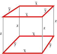
Figure 34: Almost non-geometric $T^{6}/\mathbb{Z}_{2}\times\mathbb{Z}_{2}$ which is also a Joyce orbifold. It is T-dual to $T^{6}/\mathbb{Z}_{2}\times\mathbb{Z}_{2}$.

  (i) Let us first consider the $\mathbb{Z}_{2}\times\mathbb{Z}_{2}$ orbifold generated by only $\alpha$ and $\beta$. Then, by identifying $y^{4}$ with the extra $x^{10}$ coordinate, we obtain the model in Figure 34. This is U-dual to the pure geometry $T^{6}/\mathbb{Z}_{2}\times\mathbb{Z}_{2}$ by a $y_{1}-y_{4}$ flip.

  (ii) Let us now include $\gamma$. This gives the most singular example of Joyce manifolds. The $x_{i}$ and $y_{i}$ coordinates parametrize the $S^{3}$ base and the $T^{4}$ fiber, respectively. The $(\mathbb{Z}_{2})^{3}$ orbifold group is equally well generated by $\langle\alpha,\beta,\alpha\beta\gamma\rangle$. It is important to note that the product $\alpha\beta\gamma$ does not act on the base coordinates. In principle, this could be interpreted as globally orbifolding by $(-1)^{F_{L}}$. However, this leads to problems similar to those in our earlier discussion in Section 4.1.

  It is also easy to see that U-duality does not work in this case. Compactifying M-theory on a $G_{2}$ manifold gives $\mathcal{N}=1$ supersymmetry in 4d. However, the above configuration in Type II has $\mathcal{N}=2$ supersymmetry, and therefore cannot be equivalent to the M-theory configuration. Thus we will not discuss this example any further.

• $\vec{A}=(0,0,\frac{1}{2})\sim(0,\frac{1}{2},0)\sim(\frac{1}{2},0,0)$

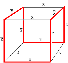
Figure 35: This modified $T^{6}/\mathbb{Z}_{2}\times\mathbb{Z}_{2}$ is also a Joyce manifold.

  The extra identification by $\gamma$ cuts the fundamental cell of $T^{6}/\mathbb{Z}_{2}\times\mathbb{Z}_{2}$ in half. The resulting base is again an $S^{3}$ which can be constructed as shown in Figure 13. The non-geometric space has the same monodromies as the model in Figure 35 that we already constructed by directly modifying the monodromies of $T^{6}/\mathbb{Z}_{2}\times\mathbb{Z}_{2}$.

  

  

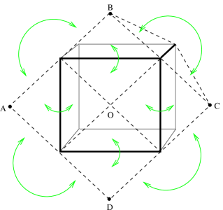
  Figure 13: (i) Fundamental domain of the base after modding by $\gamma$: half of a rhombic dodecahedron. The arrows show how the faces are identified.  (ii) Schematic picture indicating the structure of the degenerations.

• $\vec{A}=(0,\frac{1}{2},\frac{1}{2})\sim(\frac{1}{2},0,\frac{1}{2})\sim(\frac{1}{2},\frac{1}{2},0)$

  Let us consider $\vec{A}=(0,\frac{1}{2},\frac{1}{2})$, as the others are equivalent by a coordinate transformation. The action of $\alpha$ and $\beta$ generate $T^{6}/\mathbb{Z}_{2}\times\mathbb{Z}_{2}$ as usual. The third $\mathbb{Z}_{2}$ is generated by $\gamma$. It has a fixed edge which goes through two parallel faces of the cube (see Figure 14). The base is again an $S^{3}$. (The proof of this statement goes roughly as that of $T^{6}/\mathbb{Z}_{2}\times\mathbb{Z}_{2}$.)

  

  

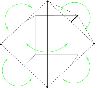
  Figure 14: (i) Half of the fundamental domain after modding by $\gamma$.  (ii) Schematic picture.

• $\vec{A}=(\frac{1}{2},\frac{1}{2},\frac{1}{2})$

  (i) Let us first omit the action of $\gamma$. This gives a somewhat simpler space with base depicted in Figure 15. It is the union of a truncated tetrahedron, plus a small tetrahedron. This base can be obtained as the intersection of fundamental domains of the two commuting $\mathbb{Z}_{2}$ actions. Both of these domains are $S^{1}$ times the square (with solid edges) depicted in Figure 2. The identification of the faces and the schematic structure of the degenerations are shown in Figure 16.

  

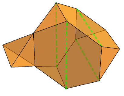
  Figure 15: The base of $T^{6}/(\mathbb{Z}_{2})^{2}$ where the generators of $\mathbb{Z}_{2}$’s include coordinate shifts. Four non-intersecting $D_{4}$ strings (dashed green lines in the middle of hexagons) curve the space into an $S^{3}$. See Figure 36 in Appendix H for a pattern that can be cut out.

  

  

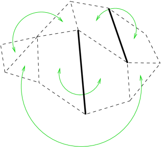
  Figure 16: (i) The base can be constructed by gluing the truncated tetrahedron (dashed lines) to itself along with a small tetrahedron. It is easy to check that the $D_{4}$ strings (solid lines) have $180^{\circ}$ deficit angle whereas the dashed lines are non-singular.  (ii) Schematic picture. The truncated tetrahedron example can roughly be understood as four linked rings of $D_{4}$ singularities. All of the rings are penetrated by two other rings which curve the space into a cylinder as they have tension 12. This forces the string to come back to itself.

  (ii) Let us now include $\gamma$ as well. The coordinate shifts in the $\mathbb{Z}_{2}$ actions make sure that the fixed edges do not intersect. The structure of the base is shown in Figure 17.

  

  

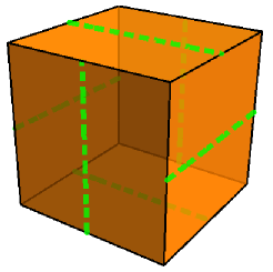
  Figure 17: (i) The base of the $(\frac{1}{2},\frac{1}{2},\frac{1}{2})$ Joyce orbifold. There are six strings located on the faces of a cube. These faces are folded up which generates the $180^{\circ}$ deficit angles.  (ii) Schematic picture. The degenerations form three rings of $D_{4}$ singularities.

4.5 Dualities between models

The two-plaquette model can be realized as $T^{6}/\mathbb{Z}_{2}\times\mathbb{Z}_{2}$ by the following orbifold action,

$$\alpha:(\theta_{1},\theta_{2},\theta_{3},\theta_{4},\theta_{5},\theta_{6}) \mapsto (-\theta_{1},-\theta_{2},-\theta_{3},-\theta_{4},\theta_{5},\theta_{6})$$

$$\beta:(\theta_{1},\theta_{2},\theta_{3},\theta_{4},x_{5},\theta_{6}) \mapsto (-\theta_{1},-\theta_{2},\theta_{3},\theta_{4},-\theta_{5},-\theta_{6})\ \times\ (-1)^{F_{L}}$$

Performing a single T-duality on $\theta_{6}$ turns $\beta$ into

$$\tilde{\beta}:(\theta_{1},\theta_{2},\theta_{3},\theta_{4},x_{5},\theta_{6})\mapsto(-\theta_{1},-\theta_{2},\theta_{3},\theta_{4},-\theta_{5},-\theta_{6})$$ (4.90)

and keeps $\alpha$ intact. We thus learn that Type IIA on the two-plaquette model is dual to Type IIB on $T^{6}/\mathbb{Z}_{2}\times\mathbb{Z}_{2}$. The details of the spectrum computation is presented in Appendix F.

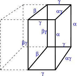
Figure 18: Monodromies of the one-shift Joyce orbifold.

Another duality is provided by considering the $\vec{A}=(\frac{1}{2},0,0)$ Joyce orbifold,

$$\begin{array}[]{llllrrrrrrrr}\alpha&:&(x_{1},x_{2},x_{3}\,|\,y_{1},y_{2},y_{3},y_{4})&\mapsto(&x_{1},&-x_{2},&-x_{3}&\,|&y_{1},&y_{2},&-y_{3},&-y_{4})\\ \beta&:&(x_{1},x_{2},x_{3}\,|\,y_{1},y_{2},y_{3},y_{4})&\mapsto(&-x_{1},&x_{2},&\frac{1}{2}-x_{3}&\,|&y_{1},&-y_{2},&y_{3},&-y_{4})\\ \gamma&:&(x_{1},x_{2},x_{3}\,|\,y_{1},y_{2},y_{3},y_{4})&\mapsto(&-x_{1},&-x_{2},&x_{3}&\,|&{-y_{1}},&y_{2},&y_{3},&-y_{4})\end{array}$$

The monodromies of the singularities in the base are shown in Figure 18 (see also Figure 13). The action of $\alpha$ and $\gamma$ creates the usual cubic structure and $\beta$ cuts the cube in half.

This $G_{2}$ orbifold can be interpreted as a Type IIA background in more than one way depending on which coordinate we choose for the $x^{10}$ circle. As discussed in the previous section, a minus sign in the $x^{10}$ direction is interpreted as $(-1)^{F_{L}}$ (this interpretation is accompanied by an inversion of fiber signs). From Figure 18 it is clear that $x^{10}=y_{2}$ or $y_{3}$ gives the one-plaquette model since in these cases $\beta$ or $\alpha$, respectively, will contain $(-1)^{F_{L}}$. On the other hand, choosing $x^{10}=y_{1}$ or $y_{4}$ gives model “U”. Since relabeling $x^{10}$ is an element of the $SL(4)$ T-duality group, these backgrounds are T-dual to each other. The spectrum is computed in Appendix G.

4.6 U-duality and affine monodromies

For usual orbifolds, it is known that the untwisted sector contains information about the singular space, whereas the twisted sectors describe resolutions (or deformations [66, 70]) thereof. It is typically said that string theory “knows” about the non-singular resolution and the number of the various particles are determined by the Hodge numbers. Here we can see this happening in a more general setup. In M-theory, the number of $\mathcal{N}=1$ vector and chiral multiplets are respectively determined by the $b_{2}$ and $b_{3}$ Betti numbers of the $G_{2}$-manifold. When U-duality works, one should obtain the same massless spectrum from the asymmetric (non-geometric) orbifold of Type IIA.

Joyce [63, 64] computed Betti numbers for blown-up $T^{7}/(\mathbb{Z}_{2})^{3}$ examples. These examples, however, contained $1/2$ shifts also in directions that were interpreted as fiber coordinates in the previous section,

$$\begin{array}[]{llllrrrrrrrr}\alpha&:&(x_{1},x_{2},x_{3}\,|\,y_{1},y_{2},y_{3},y_{4})&\mapsto(&x_{1},&-x_{2},&-x_{3}&\,|&y_{1},&y_{2},&-y_{3},&-y_{4})\\ \beta&:&(x_{1},x_{2},x_{3}\,|\,y_{1},y_{2},y_{3},y_{4})&\mapsto(&-x_{1},&x_{2},&{b_{2}}-x_{3}&\,|&y_{1},&-y_{2},&y_{3},&b_{1}-y_{4})\\ \gamma&:&(x_{1},x_{2},x_{3}\,|\,y_{1},y_{2},y_{3},y_{4})&\mapsto(&c_{5}-x_{1},&c_{3}-x_{2},&x_{3}&\,|&{-y_{1}},&y_{2},&y_{3},&c_{1}-y_{4})\end{array}$$

These shifts are recommended, otherwise one encounters “bad singularities” which can’t easily be resolved. If interpreted as a fibration, the monodromies acting on $T^{4}$ are affine transformations which also include half-shifts for some of the fiber coordinates. Although these orbifolds can readily be interpreted as non-geometric backgrounds for Type IIA, the naive U-duality map does not necessarily work and the spectrum does not match with that of M-theory.

In Appendix H, we discuss the cases of two Joyce manifolds, with two and three shifts $(b_{1},b_{2},c_{1},c_{3},c_{5})=(0,\frac{1}{2},\frac{1}{2},0,0,0)$ and $(0,\frac{1}{2},\frac{1}{2},\frac{1}{2},0,0)$. Naive U-duality works well for the three shift example and one obtains the same spectrum from the non-geometric compactification. However, the two shift example gives a different spectrum from what we expect from the Betti numbers of the $G_{2}$-manifold. The puzzle can simply be resolved by choosing a different (coassociative) fiber. Taking $\{x_{1},x_{2},y_{2},y_{3}\}$ for fiber coordinates, the $\mathbb{Z}_{2}$ transformations have no shifts in these directions and the non-geometric Type IIA spectrum indeed matches the M-theory spectrum.

5 Compactifications with ${\bf E_{n}}$ singularities

In this section, we list geometric orbifolds containing singularities other than $D_{4}$. Non-geometric modifications of these orbifolds may be done similarly to the previous section. For $D_{4}$ singularities, the constant shape of the fiber can be arbitrary. The main difference in the $E_{n}$ case is that the fiber shape is determined by the symmetry group. In practice, this means that in two dimensions $\tau=i$ or $\tau=e^{i\pi/3}$.

5.1 Orbifold limits of $K3$

Simple warm-up examples are provided by considering $T^{4}/\mathbb{Z}_{n}$ orbifolds. These have been analyzed from the F-theory point of view in [15].

The ${\bf T^{4}/\mathbb{Z}_{3}}$ orbifold. The action of the generator of the orbifold group is given by

$$\alpha:\,(z_{1},z_{2})\mapsto(e^{i\pi/3}z_{1},\,e^{-i\pi/3}z_{2})$$ (5.91)

which respects the torus identifications

$$z_{i}\sim z_{i}+1\sim z_{i}+e^{i\pi/3}$$ (5.92)

The base is $T^{2}/\mathbb{Z}_{3}$ and can be parametrized by $z_{1}$. It contains three $E_{6}$ singularities of deficit angle $4\pi/3$. The monodromy around these are given by

$$\mathcal{M}_{E_{6}}=(ST)^{2}=\left(\begin{array}[]{cc}-1&-1\\ 1&0\end{array}\right)$$ (5.93)

A fundamental cell is shown in Figure 19.

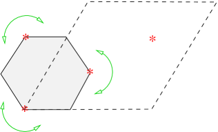
Figure 19: The base of the $T^{4}/\mathbb{Z}_{3}$ orbifold contains three $E_{6}$ singularities.

The ${\bf T^{4}/\mathbb{Z}_{4}}$ orbifold. The generator of $\mathbb{Z}_{4}$ is given by

$$\alpha:\,(z_{1},z_{2})\mapsto(iz_{1},\,-iz_{2})$$ (5.94)

with the torus identifications

$$z_{i}\sim z_{i}+1\sim z_{i}+i$$ (5.95)

The base is $T^{2}/\mathbb{Z}_{4}$. This orbifold contains two $E_{7}$ and one $D_{4}$ singularity. They have deficit angles $3\pi/2$ and $\pi$, respectively. The $E_{7}$ and $D_{4}$ monodromies are given by

$$\mathcal{M}_{E_{7}}=S=\left(\begin{array}[]{cc}0&-1\\ 1&0\end{array}\right)\qquad\mathcal{M}_{D_{4}}=\left(\begin{array}[]{cc}-1&0\\ 0&-1\end{array}\right)$$ (5.96)

A fundamental cell is shown in Figure 20.

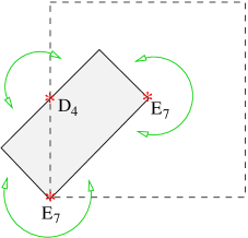
Figure 20: The base of the $T^{4}/\mathbb{Z}_{4}$ orbifold contains two $E_{7}$ and one $D_{4}$ singularities.

The ${\bf T^{4}/\mathbb{Z}_{6}}$ orbifold. The base is $T^{2}/\mathbb{Z}_{6}$. This orbifold contains $E_{8}$, $E_{6}$ and $D_{4}$ singularities. The $E_{8}$ monodromy is given by

$$\mathcal{M}_{E_{8}}=ST=\left(\begin{array}[]{cc}0&-1\\ 1&1\end{array}\right)$$ (5.97)

A fundamental cell is shown in Figure 21.

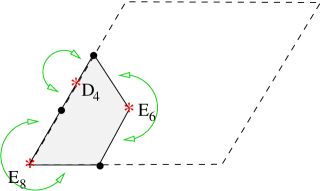
Figure 21: The base of the $T^{4}/\mathbb{Z}_{6}$ orbifold contains $E_{8}$, $E_{6}$ and $D_{4}$ singularities. The three black dots denote one non-singular point.

5.2 Example: $T^{6}/\mathbb{Z}_{3}$

We continue by discussing three dimensional examples. The simplest one is $T^{6}/\mathbb{Z}_{3}$. This is created by orbifolding the square $T^{6}$ by cyclic permutations of (complex) coordinates

$$\alpha:\,(z_{1},z_{2},z_{3})\mapsto(z_{2},z_{3},z_{1})$$ (5.98)

Clearly, this action preserves the holomorphic volume form,

$$\Omega=dz_{1}\wedge dz_{2}\wedge dz_{3}$$ (5.99)

and the Kähler form

$$\omega=\sum_{i}dz_{i}\wedge d\bar{z}_{i}$$ (5.100)

Let us now choose the real parts of $z_{i}$ for the base coordinates. Before orbifolding, the base is a cube as shown in Figure 22. The fixed loci of $\alpha$ are at $z_{1}=z_{2}=z_{3}$ that is along a diagonal. The cube has a $\mathbb{Z}_{3}$ symmetry about this diagonal, and thus the orbifolding procedure respects the torus identifications.

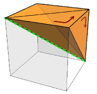
Figure 22: The base of $T^{6}/\mathbb{Z}_{3}$. The green line shows the $E_{6}$ singularity. Six triangles bound the domain. Two triangles touching the singular green line are identified by folding. Two triangles should be identified according to the orientation given by the arrows. The remaining two triangles are identified in a similar fashion.

Since $\mathbb{Z}_{3}\subset SU(2)$, this example preserves $\mathcal{N}=4$ supersymmetry in four dimensions. By making the identifications of the bounding triangles, one can check that the only singularity is $E_{6}$. It is along the diagonal which gives a closed loop in the base. Since there are no other gravitating strings to curve the space, this is a good sign that the space factorizes. In particular, we do not expect it to be an $S^{3}$.

5.3 Example: $T^{6}/\Delta_{12}$

A more complicated example is gained by orbifolding $T^{6}/(\mathbb{Z}_{2})^{2}$ by the above described cyclic permutations. These permutations do not commute with the sign flips and together they give $\Delta_{12}\subset SU(3)$. This group has the faithful representation described by the following matrices (see [71], and also [72, 73, 74]) which act on the $(z_{1},z_{2},z_{3})$ complex coordinates

$$\left(\begin{array}[]{ccc}(-1)^{p}&0&0\\ 0&(-1)^{q}&0\\ 0&0&(-1)^{p+q}\end{array}\right)\qquad\left(\begin{array}[]{ccc}0&0&(-1)^{p}\\ (-1)^{q}&0&0\\ 0&(-1)^{p+q}&0\end{array}\right)\qquad\left(\begin{array}[]{ccc}0&(-1)^{p}&0\\ 0&0&(-1)^{q}\\ (-1)^{p+q}&0&0\end{array}\right)$$ (5.101)

It can be generated by two elements,

$$\alpha:\,(z_{1},z_{2},z_{3}) \mapsto (z_{2},z_{3},z_{1})$$

$$\beta:\,(z_{1},z_{2},z_{3}) \mapsto (-z_{1},-z_{2},z_{3})$$

The fundamental domain is shown in Figure 23. There are two $E_{6}$ and four $D_{4}$ singularities in the base. They meet in $E_{6}$-$E_{6}$-$D_{4}$ and $D_{4}$-$D_{4}$-$D_{4}$ vertices. The solid angle around these vertices are $\pi/3$ and $\pi$, respectively. The base is topologically an $S^{3}$.

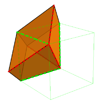
Figure 23: (i) The base of $T^{6}/\Delta_{12}$. The red and green lines indicate $E_{6}$, $D_{4}$ singularities, respectively. The other edges are non-singular. The solid green cube indicates the $D_{4}$ singularities of the original $T^{6}/(\mathbb{Z}_{2})^{2}$ orbifold. (ii) Schematic picture describing the topology of the singular lines. See Appendix H for building this polyhedron at home.

5.4 Example: $T^{6}/(\mathbb{Z}_{2})^{2}\times\mathbb{Z}_{4}$

Another example is obtained from $T^{6}/(\mathbb{Z}_{2})^{2}$ by further orbifolding it by $\mathbb{Z}_{4}$. This is possible because the rhombic dodecahedron has fourfold symmetry axes. These are the axes of the green cube in Figure 5.

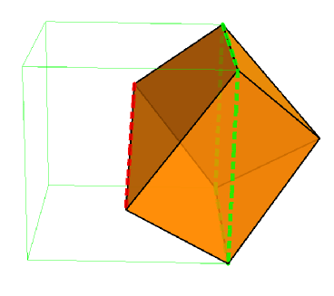
Figure 24: (i) The base of $T^{6}/(\mathbb{Z}_{2})^{2}\times\mathbb{Z}_{4}$. The red and green lines indicate $E_{7}$, $D_{4}$ singularities, respectively. The other edges are non-singular. The solid green cube indicates the $D_{4}$ singularities of the original $T^{6}/(\mathbb{Z}_{2})^{2}$ orbifold. (ii) Schematic picture describing the topology of the singular lines.

The resulting base is shown in Figure 24. There is one $E_{7}$ line which is topologically a circle. In contrast to the $T^{6}/\mathbb{Z}_{3}$ example, this happens because the other $D_{4}$ singularities curve the base and make this contractible loop a geodesic. The base only contains familiar $D_{4}$-$D_{4}$-$D_{4}$ vertices.

5.5 Example: $T^{6}/\Delta_{24}$

Our final example can be constructed by first taking $T^{6}$. Its base is a cube with opposite faces identified. We now place $E_{7}$ singularities on the twelve edges of the cube. We also add diagonal $E_{6}$ singularities as in Section 5.3. These are realized by the following matrices which act on $(z_{1},z_{2},z_{3})$ complex coordinates

$$\alpha_{E_{6}}=\left(\begin{array}[]{ccc}0&1&0\\ 0&0&1\\ 1&0&0\end{array}\right)\qquad\qquad\beta_{E_{7}}=\left(\begin{array}[]{ccc}0&-1&0\\ 1&0&0\\ 0&0&1\end{array}\right)$$ (5.102)

These generate the $\Delta_{24}$ group. Compared to $\Delta_{12}$, it also contains odd permutations of the coordinates. Since odd permutations come with an odd number of minus signs, the volume form is again invariant.

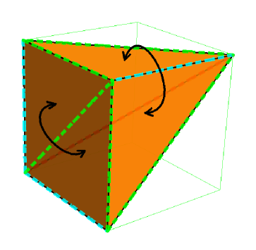
Figure 25: (i) The base of $T^{6}/\Delta_{24}$. The cyan, red and green lines indicate $E_{7}$, $E_{6}$ and $D_{4}$ singularities, respectively. (ii) Schematic picture describing the topology of the singular lines.

In Figure 25, the resulting base is shown. The green cube around the base is $1/8$ or the original base of $T^{6}$. The faces should be folded as indicated by the arrows. The rear faces touching $E_{6}$ should be also folded. This gives an $S^{3}$ with curvature concentrated in the singular lines (see the right-hand side of the figure). The base contains two types of composite vertices. One is an intersection of $E_{7}$, $E_{6}$ and $D_{4}$ edges. The other one comes from the collision of an $E_{7}$ and two $D_{4}$ singularities.

5.6 Non-geometric modifications

Having discussed the geometric structure of the fibrations with exceptional singularities, we can try to modify them into non-geometric spaces. Similarly to the examples in Section 4.2, closed loops of $D_{4}$, $E_{7}$ and $E_{8}$ singularities may be decorated with the action of $(-1)^{F_{L}}$. For example, $E_{8}={\tiny\left(\begin{array}[]{cc}0&-1\\ 1&1\end{array}\right)\oplus\left(\begin{array}[]{cc}1&0\\ 0&1\end{array}\right)}$ with $(-1)^{F_{L}}$ has the same monodromy as a composite of $A_{2}={\tiny\left(\begin{array}[]{cc}0&1\\ -1&-1\end{array}\right)}$ and a $D^{\prime}_{4}$ (which acts on the other $T^{2}\subset T^{4}$). The tension four $A_{2}$ and the tension six $D^{\prime}_{4}$ give the original deficit angle of the tension ten $E_{8}$ (see 2.2 for the Kodaira classification of singularities).

The simplest example is to add $(-1)^{F_{L}}$ to the $D_{4}$ and one of the $E_{7}$ singularities of the $T^{4}/\mathbb{Z}_{4}$ orbifold (Figure 20), or instead decorate both $E_{7}$ singularities. The $T^{4}/\mathbb{Z}_{6}$ orbifold (Figure 21) can similarly be modified by adding $(-1)^{F_{L}}$ to the $D_{4}$ and the $E_{8}$ singularities. By performing a single T-duality in the fiber, the $T^{4}/\mathbb{Z}_{4}$ monodromies can be changed to act on $SL(2)_{\rho}$ instead of $SL(2)_{\tau}$. The resulting Type IIB theory has a $D^{\prime}_{4}=D_{4}\times(-1)^{F_{L}}$ and two $E^{\prime}_{7}$ singularities. The $E^{\prime}_{7}$ corresponds to a double T-duality and thus the background is globally non-geometric, even though it has a geometric dual.

Turning to the three dimensional examples, $(-1)^{F_{L}}$ can be added to the $D_{4}$ loop of $T^{6}/\Delta_{12}$ as shown in Figure 26. This is obtained by orbifolding the last example in Figure 11. The $D_{4}$ loops or the $E_{7}$ loop of $T^{6}/(\mathbb{Z}_{2})^{2}\times\mathbb{Z}_{4}$ can similarly be modified. An example is shown in Figure 27 where a single $D_{4}$ has been changed into $D^{\prime}_{4}$ corresponding to the first example of Figure 11. A single T-duality on the geometric $T^{6}/(\mathbb{Z}_{2})^{2}\times\mathbb{Z}_{4}$ gives Type IIB with a circle of $E^{\prime}_{7}$ and thus the dual background is non-geometric. $T^{6}/\Delta_{24}$ can similarly be modified (Figure 28).

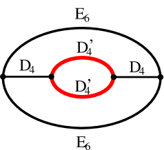
Figure 26: Non-geometric $T^{6}/\Delta_{12}$. The red lines indicate extra $(-1)^{F_{L}}$ factors.

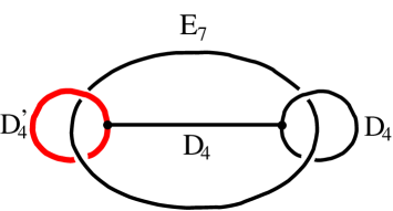
Figure 27: Non-geometric $T^{6}/(\mathbb{Z}_{2})^{2}\times\mathbb{Z}_{4}$.

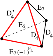
Figure 28: Non-geometric $T^{6}/\Delta_{24}$.

These spaces can serve as perturbative string backgrounds. The consistency of these vacua, however, needs further investigation.

6 Chiral Scherk-Schwarz reduction

In previous sections, we studied non-geometric spaces mainly by using a $(-1)^{F_{L}}$ monodromy around singular loci in the base. Another possibility is to have this transformation in the fiber as a Wilson line. Fields still do not depend on the fiber coordinates, and in this sense this is a (chiral) Scherk-Schwarz reduction.

6.1 One dimension

Let us consider Type IIA compactified on a circle with $(-1)^{F_{L}}$ Wilson line. This will be a one-dimensional fiber. The configuration breaks half of the supersymmetry keeping sixteen right-moving supercharges. In M-theory, $(-1)^{F_{L}}$ is described as reflection of $x^{11}$. Hence, the background lifts to M-theory as compactification on a Klein bottle [75].

An important feature of the background that one can try to exploit in the construction of non-geometric spaces is that T-duality on the circle takes Type IIA to IIA (not IIB as usual) [76, 77, 78]. Although the duality switches between the $SO(8)$ spinor and conjugate spinor representations in the right-moving sector, it also exchanges the untwisted and twisted R/NS sectors [77]. Therefore, when the circle decompactifies, the two massless 10d gravitini have different chiralities and thus the theory is still Type IIA.

At self-dual radius, the bosonic string has additional massless states and one obtains the gauge group $SU(2)\times SU(2)$. In Type II strings, these extra states are destroyed by the GSO projection and one is left with $U(1)\times U(1)$ only. With the above Wilson line, however, an extended $SU(2)\times U(1)$ gauge symmetry is obtained. In the effective theory, T-duality is part of the $SU(2)$ gauge group and thus a T-duality monodromy can be regarded as a Wilson line.

A simple two-dimensional non-geometric space is obtained by compactifying on another base circle with a monodromy that is a T-duality on the fiber circle. The consistency of this model has to be further investigated.

6.2 Two dimensions

These ideas can be generalized by considering $T^{n}$ compactifications and turning on a $(-1)^{F_{L}}$ Wilson line. This still preserves half of the supersymmetry. In order to glue spaces, only those monodromies can be considered which preserve Wilson lines, that is the “spin structure” of the $T^{n}$ fiber. Therefore, the perturbative duality group will be a proper subgroup of $O(n,n,\mathbb{Z})$.

In the following, we consider the simplest examples where the base is taken to be two dimensional and is parametrized by the complex coordinate $z$. The shape of the two-torus fiber is described by the $\tau$ complex parameter. We take the Wilson line to be along the real direction denoted by $x^{9}$. Then, along this coordinate axis, a single T-duality is possible. Applying the Buscher rules, this duality is mirror symmetry for the two-torus fiber.

Let us denote the components of an arbitrary $SL(2,\mathbb{Z})$ element $M$ by

$$M=\left(\begin{array}[]{cc}a&b\\ c&d\end{array}\right),\qquad ad-bc=1$$ (6.103)

Geometric transformations must preserve the $(-,+)$ spin structure. If $(x,y)\in\mathbb{Z}^{2}$ denotes the homotopy class of a one-cycle, then this constraint is equivalent to

$$(-1)^{x}=(-1)^{ax+by}$$ (6.104)

that is

$$(a-1)x+by=0\quad(\textrm{mod}\ 2)$$ (6.105)

Since $y$ is arbitrary, $b$ must be even. Then, $\textrm{det}\,M=1$ forces $a$ (and $d$) to be odd and the above equation is satisfied. Therefore, the geometric part of the duality group is the $\Gamma_{0}(2)\subset SL(2)$ congruence subgroup of index three. A maximal subgroup of it is $\Gamma(2)$ that contains matrices with even off-diagonal elements. $\Gamma_{0}(2)$ can be generated by $\Gamma(2)$ and the $TST^{-1}$ transformation which exchanges two cycles in the fiber. Its fundamental domain is shown in Figure 29. The full duality group contains another copy of $\Gamma_{0}(2)$ for $\rho$, and a single T-duality along $x^{9}$.

Figure 29: Fundamental domain (gray area) for the action of the $\Gamma_{0}(2)$ on the upper half-plane.

A geometric $K3$ fibration with such restricted transformations can be described by [79]

$$y^{2}+x^{4}+x^{2}w^{2}f_{4}(z)+w^{4}g_{8}(z)=0$$ (6.106)

where $(x,y,w)\in\mathbb{C}P^{2}_{1,2,1}$ and $f_{4},g_{8}$ are holomorphic sections of degree 4 and 8, respectively. The $j$-function is given by

$$j(\tau)=\frac{(f_{4}^{2}+12g_{8})^{3}}{108\,g_{8}(-f_{4}^{2}+4g_{8})^{2}}$$ (6.107)

The discriminant of the elliptic fibration vanishes generically at 16 points out of which 8 are double zeros. The moduli space is ten dimensional, in contrast to the 18 dimensional space of the cubic Weierstrass equation.

As explained in Appendix B of [79], the types of possible degenerations are $A_{n}$, $D_{n}$ and $E_{7}$. The $K3$ geometry can reach the $T^{4}/\mathbb{Z}_{2}$ orbifold limit where four $D_{4}$ singularities close the base into an $S^{2}$. The orbifold is then generated by

$$\begin{array}[]{llllrrrr}\alpha&:&(x_{1},x_{2}\,|\,y_{1},y_{2})&\mapsto(&{-x_{1}},&-x_{2}\,|&-y_{1},&-y_{2})\\ \beta&:&(x_{1},x_{2}\,|\,y_{1},y_{2})&\mapsto(&{x_{1}},&x_{2}\,|&y_{1},&\frac{1}{2}+y_{2})\end{array}$$

with $\beta$ containing $(-1)^{F_{L}}$. This is the same theory as the asymmetric orbifold limit of the $12+12^{\prime}$ model of [11]. The anomaly free $\mathcal{N}=1$ 6d spectrum contains a supergravity multiplet, nine tensor multiplets, eight vector multiplets and twenty hypermultiplets. The strong coupling limit is M-theory on a $\mathbb{Z}_{2}$ orbifold

$$(K3\times S^{1})/\left\{\sigma\cdot(y\rightarrow-y)\right\}$$ (6.109)

where $y\in[0,1)$ is the $S^{1}$ coordinate and $\sigma$ is an involution on $K3$ that acts with eight fixed points. It preserves twelve of the harmonic $(1,1)$ forms and changes the sign of the other eight harmonic $(1,1)$ forms. The spectrum computation [84] matches that of the asymmetric orbifold.

The resolved $12+12^{\prime}$ model used a doubly elliptic Weierstrass fibration over an $S^{2}$ base,

$$y^{2}=x^{3}+p_{4}(z)x+q_{6}(z)\qquad\tilde{y}^{2}=\tilde{x}^{3}+\tilde{p}_{4}(z)\tilde{x}+\tilde{q}_{6}(z)$$ (6.110)

The constants in the polynomials give a 19 dimensional moduli space. In the above orbifold limit, the complex base coordinate includes $y_{2}$ (which has the Wilson line). The $\Gamma_{0}(2)$ construction resolves the orbifold in a different ‘frame’: it chooses a different set of base coordinates, namely $x_{1}$ and $x_{2}$. It presumably slices out a different subspace in the full moduli space of the model.

Finally, T-duality along the $x^{9}$ circle can also be considered. The $\tau(z)$ and $\rho(z)$ sections can be described by considering a doubly elliptic fibration over the base. In [11], the fiber tori were independent and thus $\tau(z)$ and $\rho(z)$ were unrelated. For the present configuration with a Wilson line, however, a single T-duality can exchange them and result in more complicated non-geometric spaces. The construction of such backgrounds is left for future work.

7 Conclusions

A perturbative vacuum of string theory is specified by a conformal field theory on the worldsheet. Only in special cases will the CFT have a geometric description. Such cases include flat space, Calabi-Yau and flux compactifications, which have been studied in great detail. The development of a more systematic understanding of the set of consistent string vacua will inevitably require the study of non-geometric compactifications.

String dualities allow for the construction of string vacua that are locally geometric but not necessarily manifolds globally. Using this idea, we have constructed non-geometric compactifications preserving $\mathcal{N}=1$ supersymmetry in four dimensions. In the two dimensional case, the Weierstrass equation with holomorphic coefficients solves the equation of motion and allows for sharing the $\mathbb{Z}_{4}$ and $\mathbb{Z}_{6}$ orbifold points which is necessary for $SU(2)$ holonomy. Since an appropriate generalization of the Weierstrass equation was not at our disposal, we were only able to describe such spaces at the asymmetric orbifold point in their moduli space. A strong motivation for departing the flat-base limit is that it presumably generates a non-trivial potential for the overall volume modulus. Note that for $D_{4}$ singularities, the size of the fiber is an arbitrary free parameter which (typically) runs to large volume.

Although our explicit examples were all orbifolds, in principle, it is possible to build non-orbifold examples by means of $D_{4}$ and $E_{n}$ singularities. Since the base in this case is flat, it could be obtained by gluing various polyhedra along their faces. By carefully choosing the dihedral angles of the building blocks, one can create the appropriate deficit angles for the edges. However, it is not easy to satisfy the constraints on monodromies coming from supersymmetry and the constructions quickly get complicated. A good step in this direction would be to find a good basis of building blocks which suffice even to reconstruct the orbifold examples. By the relation discussed in Section 3.4, such spaces would presumably give new examples of $G_{2}$ manifolds.

In Appendix G, Type IIA string theory has been compactified in a non-geometric way on the “one-shift” $T^{7}/(\mathbb{Z}_{2})^{3}$ orbifold down to four dimensions. The massless spectrum is equivalent to that of the M-theory compactification on a particular resolution of this orbifold with $(b_{2},b_{3})=(16,71)$. The orbifold has, however, numerous other resolutions with very different Betti numbers [65]. It would be interesting to see whether these other resolutions arise in Type IIA by the introduction of discrete torsion (and possibly NS5-branes).

In the other direction, the result of section 3.4 shows that a general $T^{3}$-fibration with $SO(3,3,\mathbb{Z})$ T-duality monodromies has a globally geometric M-theory dual. This is striking given the difficulty of describing such creatures from the string theory point of view. More generic constructions with $SL(5)$ monodromies presumably have no duality frame where they are globally geometric.

In this paper, we have focussed on compactifications where the monodromy group was a subgroup of the perturbative duality group. There is no obstacle in principle to the extension of the monodromy group to include the full $SL(5)$ U-duality group. In this manner one can extend these techniques to include in the compactification Ramond-Ramond fields, D-branes and orientifolds, and presumably to find vacua with no massless scalars. In Appendices C and D we build confidence that such objects can be treated consistently in the semiflat approximation by rederiving from this viewpoint the Hanany-Witten brane-creation effect and the duality between M-theory on $T^{5}/\mathbb{Z}_{2}$ and type IIB on K3. Although we studied vacua of Type II string theory, the discussion can be applied to heterotic strings as well where the duality group $O(16+d,d)$ is much larger [40].

Another interesting direction is the study of leaving the large complex structure limit. Our special flat-base examples had a worldsheet description as modular invariant asymmetric orbifolds. However, in the generic case, this powerful tool is missing. Any available tools, such as the gauged linear sigma model [85], should be brought to bear on this problem.

In [12] it is proved for the $T^{2}$-fibered case that a solution in the semiflat approximation determines an exact solution. While the power of holomorphy is lacking in the $T^{3}$-fibered case, the physical motivation for this statement [11] remains. The idea is that the violations of the semiflat approximation are localized in the base, and we have a microscopic description of the degenerations, as D-branes or NS-branes or as parts of well-understood CY manifolds or orbifolds or U-duality images of these things.

It is expected that the singular edges in the base transform into ribbon graphs as we move away from the semi-flat limit [25, 86]. It seems possible that one can construct local (in the base) invariants of the fibration which give ‘NUT charges’ [87]. These invariants, which are analogous to the number of seven-branes in the stringy cosmic strings construction, appear in the [7] mirror-symmetry-covariant superpotential.

Acknowledgements

We thank Allan Adams, Henriette Elvang, Mark Hertzberg, Balázs Kőműves, Vijay Kumar, Albion Lawrence, Ruben Minasian, Dave Morrison, Washington Taylor and Alessandro Tomasiello for discussions and comments on the draft. JM acknowledges early conversations on related matters with S. Hellerman in 2003. This work is supported in part by funds provided by the U.S. Department of Energy (D.O.E.) under cooperative research agreement DE-FG0205ER41360.

Appendix A Appendix: Flat-torus reduction of type IIA to seven dimensions

The following discussion is based on [44]. Let us consider the action for the massless NS-NS fields of type II strings (in any number of dimensions)

$$S=\int dx\int dy\sqrt{-\hat{g}}\cdot e^{-\hat{\phi}}\,[R(\hat{g})+\partial_{\mu}\hat{\phi}\partial^{\mu}\hat{\phi}-\frac{1}{12}\hat{H}_{\mu\nu\rho}\hat{H}^{\mu\nu\rho}].$$ (A.111)

The $x$ coordinates label so-far-noncompact directions, and $y$ are coordinates on a $T^{d}$. We want to reduce the theory and eliminate the $y$ coordinates. Let $\mu,\nu,\ldots$ and $\alpha,\beta,\ldots$ label the corresponding indices. Taking the following ansätze,

$$\hat{g}=:\left(\begin{array}[]{cc}g_{\mu\nu}+A^{\gamma}_{\mu}A_{\nu\gamma}&\ A_{\mu\beta}\\ A_{\nu\alpha}&\ G_{\alpha\beta}\end{array}\right)$$ (A.112)

$$\phi:=\hat{\phi}-\frac{1}{2}\textrm{log det}\,G_{\alpha\beta}\qquad F^{(1)\alpha}_{\mu\nu}:=\partial_{\mu}A^{\alpha}_{\nu}-\partial_{\nu}A^{\alpha}_{\mu}$$ (A.113)

$$H_{\mu\nu\alpha}:=\hat{H}_{\mu\nu\alpha}-A^{\beta}_{\mu}\hat{H}_{\beta\nu\alpha}-A^{\beta}_{\nu}\hat{H}_{\mu\beta\alpha}$$ (A.114)

one obtains the following terms after reduction

$$S=\int dx\sqrt{-g}\,e^{-\phi}\mathcal{L}$$ (A.115)

with $\mathcal{L}=\mathcal{L}_{1}+\mathcal{L}_{2}+\mathcal{L}_{3}+\mathcal{L}_{4}$ and

$$\mathcal{L}_{1} = R+\partial_{\mu}\phi\partial^{\mu}\phi$$ (A.116)

$$\mathcal{L}_{2} = \frac{1}{4}(\partial_{\mu}G_{\alpha\beta}\partial^{\mu}G^{\alpha\beta}-G^{\alpha\beta}G^{\gamma\delta}\partial_{\mu}B_{\alpha\gamma}\partial^{\mu}B_{\beta\delta})$$ (A.117)

$$\mathcal{L}_{3} = -\frac{1}{4}g^{\mu\rho}g^{\nu\lambda}(G_{\alpha\beta}F^{(1)\alpha}_{\mu\nu}F^{(1)\beta}_{\rho\lambda}+G^{\alpha\beta}H_{\mu\nu\alpha}H_{\rho\lambda\beta})$$ (A.118)

$$\mathcal{L}_{4} = -\frac{1}{12}H_{\mu\nu\rho}H^{\mu\nu\rho}$$ (A.119)

In order to see the $SO(d,d,\mathbb{Z})$ symmetry, one introduces the $2d\times 2d$ matrix

$$M=\left(\begin{array}[]{cc}G^{-1}&G^{-1}B\\ BG^{-1}&\ \ G-BG^{-1}B\end{array}\right)$$ (A.120)

This symmetric matrix is in $SO(d,d)$, that is

$$M^{T}\eta M=\eta\qquad\qquad\eta\equiv\left(\begin{array}[]{cc}0&1_{2\times 2}\\ 1_{2\times 2}&0\end{array}\right)$$ (A.121)

$M$ is positive definite which can be seen as follows. First notice that the above properties of $M$ imply that the eigenvalues are present with their reciprocals,

$$M\vec{v}=\lambda\vec{v}\qquad\Longrightarrow\qquad M(\eta\vec{v})=\lambda^{-1}(\eta\vec{v})$$ (A.122)

Let us now turn off the B-field. The eigenvalues of $M(B=0)$ are simply the eigenvalues of $G$ and the reciprocals: $\lambda_{i}$ and $1/\lambda_{i}$, all positive. As we turn on the B-field, we do not expect any singularities in the eigenvalues since $M$ is quadratic in $B$. Therefore the eigenvalues remain positive.

Let us introduce

$$H_{\mu\nu\alpha}=\partial_{\mu}B_{\nu\alpha}-\partial_{\nu}B_{\mu\alpha}=:F^{(2)}_{\mu\nu\alpha}$$ (A.123)

we can collect the field strength in the following $SO(d,d)$ vector

$$\mathcal{F}^{i}_{\mu\nu}:=\binom{F^{(1)\alpha}_{\mu\nu}}{F^{(2)}_{\mu\nu\beta}}$$ (A.124)

With these ingredients, one can explicitly see the $SO(3,3)$ invariance of the Lagrangian. $\mathcal{L}_{1}$ is trivially invariant. The kinetic terms can be written as

$$\mathcal{L}_{2}=\frac{1}{8}\textrm{Tr}(\partial_{\mu}M^{-1}\partial^{\mu}M)$$ (A.125)

Also,

$$\mathcal{L}_{3}=-\frac{1}{4}\mathcal{F}^{i}_{\mu\nu}(M^{-1})_{ij}\mathcal{F}^{\mu\nu j}$$ (A.126)

which is invariant. Since $H_{\mu\nu\rho}$ does not change under the duality group, $\mathcal{L}_{4}$ is also invariant.

Appendix B Appendix: Semi-flat vs. exact solutions

In this section we compare the exact supergravity solutions to the semi-flat description. We study the approximation through the example of an NS5-brane. NS5-branes are parametrically heavier than D-branes and they curve spacetime even to zeroth approximation.

Semi-flat approximation. In order for the semi-flat machinery to work, we need to compactify the transverse space. The transverse space is now a two-torus fiber over a complex $z$-plane. The NS5-brane can be described by a $\rho\mapsto\rho+1$ monodromy around a singular point in the $z$-plane. This can be achieved by the following solution [12]

$$\rho(z)\sim\frac{1}{2\pi i}\textrm{log}(z)$$ (B.127)

As we approach the brane ($|z|\rightarrow 0$), the torus fiber decompactifies,

$$V_{\textrm{fiber}}\sim\rho_{2}\sim-\textrm{log}|z|$$ (B.128)

Since the eight dimensional dilaton can be set to constant [11], the ten dimensional dilaton is (Appendix A)

$$2\phi=\frac{1}{2}\textrm{log det}\,G_{\alpha\beta}$$ (B.129)

that is

$$e^{2\phi}=V_{\textrm{fiber}}$$ (B.130)

and the dilaton grows near the origin.

Exact NS5 solution. If $x^{m}$ are transverse to the NS5-brane and $x^{\mu}$ are tangent to it, then the exact non-compact classical solution in the string frame is given by (see [88], page 183)

$$G_{mn}=e^{2\phi}\,\delta_{mn} G_{\mu\nu}=\eta_{\mu\nu}$$ (B.131)

$$H_{mnp}=-\epsilon_{mnp}^{q}\partial_{q}\phi e^{2\phi}=e^{2\phi(\infty)}+\frac{1}{2\pi^{2}r^{2}}$$ (B.132)

where $r^{2}=\sum(x^{m})^{2}$. The geometry has an infinite throat: the origin $x^{m}=0$ is at infinite distance and the angular $S^{3}$ approaches an asymptotic constant size. In the Einstein frame ($G^{\textrm{Einstein}}_{\mu\nu}=e^{-\phi/2}\,G^{\textrm{string}}_{\mu\nu}$), the singularity is at finite distance. There is a growing dilaton in the throat and string perturbation theory eventually breaks down. At infinity, the metric asymptotes to flat space.

In order to derive the semi-flat solution from the exact one, we need to compactify the latter on a two-torus. In the covering space, this amounts to placing an infinite number of NS5-branes in a 2d lattice $\Lambda$ in the 4d transverse space. For sake of simplicity, we take this to be a square lattice. Since the branes are BPS, the solution comes from simple superposition,

$$e^{2\phi(x)}=e^{2\phi(\infty)}+\frac{1}{2\pi^{2}}\sum_{(n,m)\in\Lambda}\left(\frac{1}{|x-x_{n,m}|^{2}}-\frac{1}{|x_{n,m}|^{2}}\right)$$ (B.133)

where $x$ and $x_{n,m}$ are four-vectors, the latter one denoting the positions of the lattice points parametrized by two integers $n$ and $m$.

If we neglect distances smaller than the lattice spacing, then we obtain

$$e^{2\phi(z,\bar{z})}=e^{2\phi(\infty)}+\frac{1}{2\pi^{2}}\sum_{n,m}\left(\frac{1}{z\bar{z}+n^{2}+m^{2}}-\frac{1}{n^{2}+m^{2}}\right)$$ (B.134)

where we introduced a complex $z$ coordinate perpendicular to the 2d lattice. This is the base coordinate. This expression can now be compared to the semi-flat solution. If we denote $r\equiv|z|$, then taking the derivative w.r.t $r$ gives for the semi-flat solution

$$\partial_{r}\,e^{2\phi_{\textrm{semi-flat}}}=\partial_{r}\,V_{\textrm{fiber}}\sim-\frac{1}{r}$$ (B.135)

For our expression,

$$\partial_{r}\,e^{2\phi(z,\bar{z})}=-\frac{1}{2\pi^{2}}\sum_{n,m}\frac{2r}{r^{2}+n^{2}+m^{2}}\approx-\int du\,dv\frac{2r}{r^{2}+u^{2}+v^{2}}\sim-\frac{1}{r}$$ (B.136)

where we approximated the sum by an integral. Thus, we reproduced the semi-flat dilaton from the exact one.

Although the semi-flat approximation reproduces the qualitative features of the exact solution, due to the partially compactified transverse space, we have to deal with another problem. The function (B.127) is valid only close to the brane. A semi-flat solution that extends to the entire complex plane may be given by means of the $j$-function. This solution suffers from the problem of orbifold points as we described in Section 2.2 and it is not possible to describe a single NS5-brane consistently. The exact solution avoids this problem by roughly speaking going to the limit very close to the brane (in the $z$-plane) compared to the size of the fiber. Hence, any possible orbifold points are pushed to an infinite distance (in the base) and thus are invisible.

example	potential
flat space	$V(\vec{x})=\frac{1}{|\vec{x}|}$
Taub-NUT	$V(\vec{x})=1+\frac{1}{|\vec{x}|}$
Eguchi-Hanson	$V(\vec{x})=\frac{1}{|\vec{x}-\vec{x_{1}}|}+\frac{1}{|\vec{x}-\vec{x_{2}}|}$

Table 3: Some well-known examples for the Gibbons-Hawking ansatz.

The Gibbons-Hawking ansatz. A perhaps more visual comparison of the semi-flat and exact metrics is possible through the ansatz,

$$ds^{2}=V(\vec{x})d\vec{x}^{2}+V(\vec{x})^{-1}\,(dt+\vec{A}\cdot d\vec{x})^{2}$$ (B.137)

where $\vec{A}$ is given through $\vec{\nabla}\times\vec{A}=\vec{\nabla}V$. This defines a circle fibration over a three dimensional base parametrized by $\vec{x}$. A semi-flat solution for a degenerating fiber is given through

$$\tau(z)\sim\frac{1}{2\pi i}\textrm{log}(z)$$ (B.138)

This corresponds to [92]

$$V=\tau_{2}=-\frac{1}{2\pi}\textrm{log}\,|z|$$ (B.139)

$$A_{x}=\tau_{1}=\frac{1}{4\pi i}\textrm{log}(z/\bar{z})\qquad A_{z}=0\qquad A_{\bar{z}}=0$$ (B.140)

where the 3d $\vec{x}$ space has been decomposed into $(x,z,\bar{z})$. This gives a singular metric which is translationally invariant in the $x$ direction.

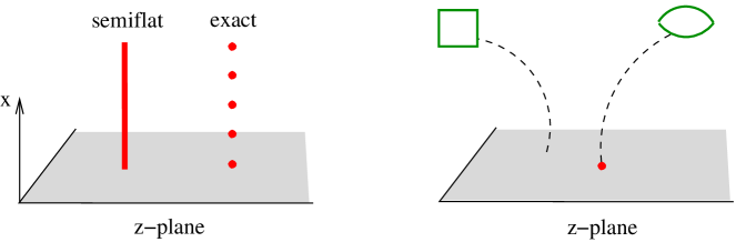
Figure 30: (i) Comparing semi-flat and exact metrics for around degenerating fibers. The base is 3d, parametrized by the periodic $x$ coordinate and the complex $z$-plane. The red line / red dots indicate where the $S^{1}$ fiber vanishes. Translational invariance of the semi-flat solution is replaced by periodicity of the exact metric in the $x$ direction.  (ii) The same (exact) metric from a different viewpoint. The horizontal direction in the torus fiber is the $x$ coordinate. The torus pinches at the degeneration point (red dot) in the 2d base. Topologically, the singular fiber is an $S^{2}$ with two points glued together. This replaces the degenerating $\tau_{2}\rightarrow\infty$ torus of the semi-flat solution.

The exact non-singular hyper-Kähler metric is not translationally invariant, but periodic.

$$V=\frac{1}{4\pi}\sum_{n=-\infty}^{\infty}\left(\frac{1}{\sqrt{(x-n)^{2}+z\bar{z}}}-\frac{1}{|n|}\right)+\textrm{const.}$$ (B.141)

In Figure 30 (i), red dots indicate where this potential is singular. An $S^{3}$ (the “throat”) close to such a degeneration point can be seen as a Hopf-fibration with fiber $t$ above the $S^{2}$ surrounding the singularity. On the right-hand side of Figure 30, we see again the SYZ-like fibration with a two-torus fiber above the complex plane. The torus fiber degenerates into a “pillow” above a codimension two locus.

It is possible to glue an approximate $K3$ metric from 24 such patches. For details, see [16]. A more conventional way to obtain a smooth approximate metric is to start with the singular $T^{4}/\mathbb{Z}_{2}$ orbifold and blow up the 16 fixed points. This is possible by cutting out a small neighborhood (whose boundary is homeomorphic to $\mathbb{R}\mathbb{P}^{3}$) around the fixed point and gluing there an Eguchi-Hanson space. This is the unique smooth hyper-Kähler metric which asymptotes to $\mathbb{C}^{2}/\mathbb{Z}_{2}$.

Appendix C Appendix: The Hanany-Witten effect from the semiflat approximation

The Hanany-Witten effect [93] is an interesting phenomenon of brane creation. It can be used to construct brane configurations that realize four dimensional $\mathcal{N}=1$ supersymmetric gauge theories [94] which exhibit Seiberg duality. This duality relates two different gauge theories which give the same infrared physics [95]. In string theory, it is realized in a very geometric way: as the branes move around, new branes appear which can change the rank of the gauge group in the 4d theory.

The Hanany-Witten setup co tains D4-branes stretched between NS5-branes in the presence of D6-branes. The D6, D4 and NS5 are magnetically charged under $C^{(1)}$, $C^{(3)}$ and $B$, respectively. The branes that we are going to use have the following orientations

	0	1	2	3	4	5	6	7	8	9
NS5	x	x	x	x	x					x
D6	x	x	x	x		x		x	x
D4	x	x	x	x			x

Table 4: Branes in the Hanany-Witten setup. $456$ are the base, $789$ are the fiber coordinates.

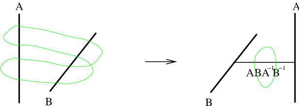
Figure 31: Hanany-Witten brane creation mechanism. $A$ and $B$ are the monodromies of the NS5- and D6-branes, respectively. As the two branes pass through each other, a new brane appears with a monodromy around the green circle (see right-hand side). This monodromy can be easily computed in the original configuration (left-hand side) where the green path was a deformed loop around the two branes. The result is $ABA^{-1}B^{-1}$ which is simply the monodromy of a D4-brane.

Let us now consider an NS5-brane and a D6-brane as in the left-hand side of Figure 31. As the two branes pass though each other, a new brane is created. In order to verify that it is indeed a D4-brane, we need to determine its monodromy. Ramond-Ramond charges $(C_{7},C_{8},C_{9},C_{789})$ transform in the dual fundamental representation of $SL(4)$, which means that we have to use the transposed monodromy matrices.

The NS5 monodromy,

$$A=\mathcal{M}_{\textrm{NS5}}=\left(\begin{array}[]{rrrr}1&0&0&0\\ 0&1&0&0\\ 0&0&1&1\\ 0&0&0&1\end{array}\right)$$ (C.142)

and the D6 monodromy

$$B:\ C_{9}\mapsto C_{9}+1$$ (C.143)

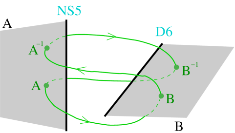
Figure 32: Determining the monodromy around the green loop by means of 2d branch cuts.

From these ingredients, we need to determine the monodromy along the green loop in the left-hand side of Figure 31. A moment’s thought will convince the reader that it is the (group-theoretic) commutator, $ABA^{-1}B^{-1}$. This is best seen by choosing “branch cut planes” that start from the branes and studying how the green loop intersects these (see Figure 32).

Finally, the commutator can be computed

$$ABA^{-1}B^{-1}:\ C_{789}\mapsto C_{789}+1$$ (C.144)

which is the monodromy of a D4-brane.

Appendix D Appendix: Type IIA on ${\bf T^{5}/\mathbb{Z}_{2}}$ and Type IIB on ${\bf S^{1}\times K3}$

Type IIA string theory on $T^{5}/\mathbb{Z}_{2}$ has been conjectured to be equivalent to Type IIB on $S^{1}\times K3$ [109, 110]. We study this equivalence by means of the semi-flat machinery.

The IIA orientifold $T^{5}/\mathbb{Z}_{2}$ is generated by the action $\alpha\cdot\Omega$ that reverses the sign of all the circles,

$$\alpha:(x^{5},x^{6},x^{7},x^{8},x^{9})\mapsto(-x^{5},-x^{6},-x^{7},-x^{8},-x^{9})$$ (D.145)

and changes the parity of the world-sheet. There are 32 D4-branes located at the fixed points which cancel the RR tadpoles.

We cast the geometry in a fibration structure as follows. The 2d base coordinates will be $x^{5}$ and $x^{6}$. Since $\alpha$ inverts these coordinates, the base becomes $T^{2}/\mathbb{Z}_{2}$, i.e. a semi-flat $S^{2}$. Over this sphere there is a $T^{3}$ fiber parametrized by $x^{7}$, $x^{8}$ and $x^{9}$. The fiber degenerates at four points in the base. These singularities have a deficit angle of $180^{\circ}$ (tension six, like $D_{4}$). The monodromy around the singular points in the base is then

$$\mathcal{M}=R_{789}\cdot\Omega$$ (D.146)

where $R_{i}$ is reflection of the i-th coordinate, $\Omega$ is the world-sheet parity transformation. This monodromy already includes the monodromies of eight D4-branes which cancel the RR-charges of the O4-plane. This is analogous to the orientifold limit of F-theory where the O7-plane monodromy is

$$\mathcal{M}_{\textrm{O7}^{-}}=-T^{-4}\qquad\textrm{with}\quad T=\mathcal{M}_{\textrm{D7-brane}}=\left(\begin{array}[]{rr}1&1\\ 0&1\end{array}\right)$$ (D.147)

which combines with the monodromy of the four D7-branes ($T^{4}$) to cancel the RR-charge. The final monodromy matrix is then diagonal.

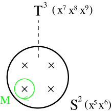
Figure 33: $T^{5}/\mathbb{Z}_{2}$ as a fibration over $S^{2}$. The geometric $T^{3}$ fiber gets promoted to $T^{5}$ by adding $x^{10}$ and the M-theory circle $x^{11}$. The monodromy $\mathcal{M}$ then acts on this $T^{5}$.

What is $\mathcal{M}$ explicitly? Type IIB orientifolds at strong coupling can be described by F-theory. As already mentioned in Section 3.4, the torus fiber of F-theory is analogous to the $x^{11}-x^{10}$ coordinates in our case. Therefore, perturbative dualities are not sufficient for determining the monodromy around the orientifold fixed points and the $x^{11}$ coordinate should be included in the discussion. In the following, we determine the $5\times 5$ U-duality monodromy matrices in the basis of $x^{7}-x^{8}-x^{9}-x^{11}-x^{10}$.

Reflection has an immediate interpretation in the vector representation of $SO(3,3)$. Since inversion of a coordinate exchanges the two spinors that have different chirality, only an even number of reflections give a symmetry of Type IIA. For instance, reflection of both $x^{7}$ and $x^{8}$ can be represented by

$$R_{78}=\textrm{diag}(-1,-1,+1,-1,-1,+1)\in SO(3,3)$$ (D.148)

which inverts the momentum and the winding as well. It has the spinor representation

$$R_{78}=\textrm{diag}(-1,-1,+1,+1)\in SL(4)$$ (D.149)

Odd number of reflections must be accompanied with other internal symmetries. However, we can still determine the corresponding monodromies, keeping in mind that we have to combine them with other symmetries. The relevant reflection is that of $x^{7}-x^{8}-x^{9}$ which gives

$$R_{789}=\textrm{diag}(-1,-1,-1,+1,-1)$$ (D.150)

The inversion of $x^{10}$ comes about because the three coordinate reflections change the sign of the Levi-Civita pseudotensor that we used to convert the three-form field into a vector.

Let us consider the world-sheet parity transformation $\Omega$. In the Type IIA language, under this transformation the metric, the dilaton and the Ramond-Ramond one-form are even, whereas the B-field and the three-form are odd. In M-theory language this means that the three-form switches sign. From this, one can determine the $\Omega$ monodromy to be

$$\Omega=\,\pm\,\textrm{diag}(+1,+1,+1,+1,-1)$$ (D.151)

In order to fix the overall sign, let us consider an O6 orientifold plane. It is obtained by the action of $R_{7\,8\,9\,11}$ which reduces to $(-1)^{F_{L}}\Omega R_{789}$ in the IIA limit ([111], see also [68, 112]).

Since $(-1)^{F_{L}}$ changes the signs of the RR-fields, the corresponding monodromy is easy to determine,

$$(-1)^{F_{L}}=\textrm{diag}(-1,-1,-1,+1,-1)$$ (D.152)

Since

$$R_{7\,8\,9\,11}=\textrm{diag}(-1,-1,-1,-1,+1)$$ (D.153)

we obtain

$$\Omega=\textrm{diag}(-1,-1,-1,-1,+1)$$ (D.154)

From these ingredients we can now write down the explicit form of the monodromy in the $T^{5}/\mathbb{Z}_{2}$ orientifold of Type IIA,

$$\mathcal{M}=R_{789}\cdot\Omega=\textrm{diag}(+1,+1,+1,-1,-1)$$ (D.155)

where we immediately recognize the monodromy of a (conjugate) $D_{4}$ singularity

$$\mathcal{M}=U\underbrace{\textrm{diag}(-1,-1,+1,+1,+1)}_{R_{\tilde{7}\tilde{8}}}U^{-1}$$ (D.156)

Therefore by flipping $x^{7}-x^{11}$ and $x^{8}-x^{10}$, we obtain Type IIA on K3. The volume of the $T^{2}$ fiber is the inverse of the volume of the original $T^{3}$ fiber,

$$vol(T^{2})=R_{\tilde{7}}R_{\tilde{8}}=R_{11}R_{10}=R_{11}\frac{1}{R_{7}R_{8}R_{9}R_{11}}=\frac{1}{R_{7}R_{8}R_{9}}=\frac{1}{vol(T^{3})}$$ (D.157)

Here we used the fact that the $T^{5}$ torus has unit volume in appropriate units.

Finally, by T-dualizing the spectator $x^{9}$ ($R_{\tilde{9}}=1/R_{9}$), we arrive at the final equivalence,

$$\textrm{Type IIA on}\ T^{5}/\mathbb{Z}_{2}\ \textrm{orientifold}\quad\cong\quad\textrm{Type IIB on}\ K3\times S^{1}$$ (D.158)

Appendix E Appendix: List of asymmetric orbifolds

In this Appendix, we list the asymmetric orbifold actions that realize the almost non-geometric spaces of Section 4.2. The one-plaquette example was described in Section 4.3. We use the following trick [11]: some of the compact dimensions are “unfolded” and compactified back with an asymmetric action. The complexity of the model depends on how many dimensions have to be unfolded.

Two-plaquette model

$$\alpha:(\theta_{1},\theta_{2},\theta_{3},\theta_{4},\theta_{5},\theta_{6}) \mapsto (-\theta_{1},-\theta_{2},-\theta_{3},-\theta_{4},\theta_{5},\theta_{6})$$

$$\beta:(\theta_{1},\theta_{2},\theta_{3},\theta_{4},\theta_{5},\theta_{6}) \mapsto (-\theta_{1},-\theta_{2},\theta_{3},\theta_{4},-\theta_{5},-\theta_{6})\ \times\ (-1)^{F_{L}}$$

Model “U”

$$\alpha:(\theta_{1},\theta_{2},\theta_{3},\theta_{4},x_{5},\theta_{6}) \mapsto (-\theta_{1},-\theta_{2},-\theta_{3},-\theta_{4},x_{5},\theta_{6})\ \times\ (-1)^{F_{L}}$$

$$\gamma_{1}:(\theta_{1},\theta_{2},\theta_{3},\theta_{4},x_{5},\theta_{6}) \mapsto (\theta_{1},\theta_{2},-\theta_{3},-\theta_{4},-x_{5},-\theta_{6})\ \times\ (-1)^{F_{L}}$$

$$\gamma_{2}:(\theta_{1},\theta_{2},\theta_{3},\theta_{4},x_{5},\theta_{6}) \mapsto (\theta_{1},\theta_{2},-\theta_{3},-\theta_{4},L-x_{5},-\theta_{6})$$

Model “L”

$$\alpha_{1}:(x_{1},\theta_{2},\theta_{3},\theta_{4},x_{5},\theta_{6}) \mapsto (-x_{1},-\theta_{2},-\theta_{3},-\theta_{4},x_{5},\theta_{6})\ \times\ (-1)^{F_{L}}$$

$$\alpha_{2}:(x_{1},\theta_{2},\theta_{3},\theta_{4},x_{5},\theta_{6}) \mapsto (L-x_{1},-\theta_{2},-\theta_{3},-\theta_{4},x_{5},\theta_{6})$$

$$\gamma_{1}:(x_{1},\theta_{2},\theta_{3},\theta_{4},x_{5},\theta_{6}) \mapsto (x_{1},\theta_{2},-\theta_{3},-\theta_{4},-x_{5},-\theta_{6})\ \times\ (-1)^{F_{L}}$$

$$\gamma_{2}:(x_{1},\theta_{2},\theta_{3},\theta_{4},x_{5},\theta_{6}) \mapsto (x_{1},\theta_{2},-\theta_{3},-\theta_{4},L-x_{5},-\theta_{6})$$

Model “X”

$$\alpha_{1}:(x_{1},\theta_{2},x_{3},\theta_{4},x_{5},\theta_{6}) \mapsto (-x_{1},-\theta_{2},-x_{3},-\theta_{4},x_{5},\theta_{6})$$

$$\alpha_{2}:(x_{1},\theta_{2},x_{3},\theta_{4},x_{5},\theta_{6}) \mapsto (L-x_{1},-\theta_{2},-x_{3},-\theta_{4},x_{5},\theta_{6})\ \times\ (-1)^{F_{L}}$$

$$\alpha_{3}:(x_{1},\theta_{2},x_{3},\theta_{4},x_{5},\theta_{6}) \mapsto (-x_{1},-\theta_{2},L-x_{3},-\theta_{4},x_{5},\theta_{6})\ \times\ (-1)^{F_{L}}$$

$$\alpha_{4}:(x_{1},\theta_{2},x_{3},\theta_{4},x_{5},\theta_{6}) \mapsto (L-x_{1},-\theta_{2},L-x_{3},-\theta_{4},x_{5},\theta_{6})$$

$$\gamma_{1}:(x_{1},\theta_{2},x_{3},\theta_{4},x_{5},\theta_{6}) \mapsto (x_{1},\theta_{2},-x_{3},-\theta_{4},-x_{5},-\theta_{6})$$

$$\gamma_{2}:(x_{1},\theta_{2},x_{3},\theta_{4},x_{5},\theta_{6}) \mapsto (x_{1},\theta_{2},L-x_{3},-\theta_{4},-x_{5},-\theta_{6})\ \times\ (-1)^{F_{L}}$$

$$\gamma_{3}:(x_{1},\theta_{2},x_{3},\theta_{4},x_{5},\theta_{6}) \mapsto (x_{1},\theta_{2},-x_{3},-\theta_{4},L-x_{5},-\theta_{6})\ \times\ (-1)^{F_{L}}$$

$$\gamma_{4}:(x_{1},\theta_{2},x_{3},\theta_{4},x_{5},\theta_{6}) \mapsto (x_{1},\theta_{2},L-x_{3},-\theta_{4},L-x_{5},-\theta_{6})$$

Appendix F Appendix: Spectrum of ${\bf T^{6}/\mathbb{Z}_{2}\times\mathbb{Z}_{2}}$ and the two-plaquette model

For comparison and as a warm-up exercise, in this Appendix we review the details of the computation of massless spectra for ${T^{6}/\mathbb{Z}_{2}\times\mathbb{Z}_{2}}$ [66] and for its T-dual, the two-plaquette model. We will work in the RNS formalism. The compactification preserves $\mathcal{N}=2$ supersymmetry in four dimensions. The $\mathcal{N}=2$ multiplets are listed in the Table 5.

hypermultiplet	2 fermions,  4 scalars
vector multiplet	vector,  2 fermions,  2 scalars
supergravity multiplet	graviton,  2 gravitini,  vector

Table 5: Massless $\mathcal{N}=2$ multiplets in four dimensions (Weyl fermions and real scalars).

The massless spectrum of $T^{6}/\mathbb{Z}_{2}\times\mathbb{Z}_{2}$

• untwisted sector

  The spectrum contains the states that are invariant under the orbifold projection. Each of the orbifold group generators invert four spacetime coordinates. The action should also be specified on the fermions. We use the following convention,

  $$\alpha:(\pi,-\pi,0)\quad\beta:(-\pi,0,\pi)\quad\alpha\beta:(0,-\pi,\pi)$$ (F.159)

  The action of these elements on the states are summarized in the following table,

  sector	state	$\alpha$, $\beta$, $\alpha\beta$ charge
  $NS$	$\psi^{\mu}_{-1/2}|0;k\rangle$	$+++$
  	$\psi^{4,5}_{-1/2}|0;k\rangle$	$--+$
  	$\psi^{6,7}_{-1/2}|0;k\rangle$	$-+-$
  	$\psi^{8,9}_{-1/2}|0;k\rangle$	$+--$
  $R$	$|\textrm{\tiny gso}+++\rangle,\ |\textrm{\tiny gso}---\rangle$	$+++$
  	$|\textrm{\tiny gso}++-\rangle,\ |\textrm{\tiny gso}--+\rangle$	$+--$
  	$|\textrm{\tiny gso}+-+\rangle,\ |\textrm{\tiny gso}-+-\rangle$	$-+-$
  	$|\textrm{\tiny gso}+--\rangle,\ |\textrm{\tiny gso}-++\rangle$	$--+$

  Table 6: Untwisted NS and R sectors. In the R sector, only the spins of compact complex dimensions are indicated. The remaining one is determined by the GSO projection as indicated by the “gso” label. This depends on whether it’s the left or right R sector.

  sector	fields
  $NS_{-}/NS_{-}$	$G_{\mu\nu}$, $B_{\mu\nu}$, dilaton, 12 real scalars
  $NS_{-}/R_{+}$	gravitino, 7 Weyl fermions
  $R_{-}/NS_{-}$	gravitino, 7 Weyl fermions
  $R_{-}/R_{+}$	4 vectors, 4 cx. scalars

  Table 7: Untwisted sectors. The signs show the matter GSO projection (which, due to the superghost contributions, differ from the full GSO in the NS sectors).

  These states combine into 1 supergravity multiplet, 3 vector multiplets and 4 hypermultiplets according to Table 5.

  
  

• twisted sectors

  There are $16+16+16=48$ fixed tori under $\alpha$, $\beta$ and $\alpha\beta$. The zero-point energies vanish and both NS and R sectors have zero modes in the twisted and untwisted directions, respectively.

  sector	state	$\alpha$, $\beta$, $\alpha\beta$ charge
  $NS$	$|\,.\ .++\rangle$	$-i,\ i,\ 1$
  	$|\,.\ .--\rangle$	$i,\ -i,\ 1$
  $R$	$|\textrm{\tiny gso}+.\ .\ \rangle$	$i,\ -i,\ 1$
  	$|\textrm{\tiny gso}-.\ .\ \rangle$	$-i,\ i,\ 1$

  Table 8: $(\alpha\beta)$-twisted NS and R sectors. The other twisted sectors are analogous. The dots indicate half-integer moded oscillators which generate massive states.

  sector	fields
  $NS_{+}/NS_{+}$	cx. scalar
  $NS_{+}/R_{-}$	Weyl fermion
  $R_{+}/NS_{+}$	Weyl fermion
  $R_{+}/R_{-}$	vector

  Table 9: Each twisted sector gives an $\mathcal{N}=2$ vector multiplet.

  These states give 48 vector multiplets.

Vertex operators are local with respect to the eight supercharges

$$e^{-\varphi/2}e^{\frac{i}{2}(H_{0}\pm H_{1})\pm\frac{i}{2}(H_{2}+H_{3}+H_{4})}$$ (F.160)

$$e^{-\tilde{\varphi}/2}e^{\frac{i}{2}(\tilde{H}_{0}\pm\tilde{H}_{1})\pm\frac{i}{2}(\tilde{H}_{2}+\tilde{H}_{3}+\tilde{H}_{4})}$$ (F.161)

In $\mathcal{N}=2$ language, this gives altogether one supergravity, 51 vector and 4 hypermultiplets. This is consistent with the expectations that Type IIA compactified on a Calabi-Yau should result in $h^{1,1}=51$ vector multiplets and $h^{2,1}+1=4$ hypermultiplets [66].

In $\mathcal{N}=1$ language, a hyper is two chirals, a vector is a vector+chiral, and the supergravity multiplet is a gravity + gravitino multiplet as seen from Table 10. Therefore, we obtain a gravity, a gravitino, 51 vector and 59 chiral multiplets.

chiral multiplet	fermion,  2 scalars
vector multiplet	vector,  fermion
gravitino multiplet	gravitino,  vector
gravity multiplet	graviton,  gravitino

Table 10: Massless $\mathcal{N}=1$ multiplets in four dimensions (Weyl fermions and real scalars).

The massless spectrum of the two-plaquette model. The theory is described in Section 4.2 (see Figure 11 for the singularity structure). As discussed in Section 4.5, Type IIA on this background is T-dual to Type IIB on ordinary $T^{6}/\mathbb{Z}_{2}\times\mathbb{Z}_{2}$. As a further exercise, we compute the spectrum. The theory is defined as a $\mathbb{Z}_{2}\times\mathbb{Z}_{2}$ orbifold generated by $\alpha$ and $\beta$, similarly to the previous section. In this case, however, $\alpha$ includes the action of $(-1)^{F_{L}}$. In the RNS formalism, $(-1)^{F_{L}}$ does not act directly on the worldsheet fields. It changes the sign of the left-moving spin-fields and hence acts as charge conjugation on RR-fields. The GSO projection is switched in left-moving sectors twisted by $\mathcal{R}\cdot(-1)^{F_{L}}$ compared to sectors twisted by $\mathcal{R}$ only. (Here $\mathcal{R}$ inverts four spacetime coordinates.) This can be deduced using the equivalence of the RNS and Green-Schwarz formalisms. In the latter description, $(-1)^{F_{L}}$ changes the sign of the $\theta^{a}$ left-moving world-sheet spinor fields in the light-cone gauge (for a review, see e.g. [113]).

We again need to impose GSO and orbifold invariance. In the twisted sectors, an ambiguity arises: one can keep even or odd states under the action of a certain $\mathbb{Z}_{2}$ generator. The choices are constrained by modular invariance. The signs are shown in Table 11.

	$\alpha$-twisted	${\bf\beta}$-twisted	${\bf\alpha\beta}$-twisted
$P_{\alpha}$	$-$	$+$	$-$
$P_{\beta}$	$+$	$+$	$+$
$P_{\alpha\beta}$	$-$	$+$	$-$

Table 11: Signs of projections in various twisted sectors.

The signs on the diagonal are directly related to the coloring of the edges (Figure 11). Perhaps the off-diagonal signs can be encoded in faces of the SYZ graph.

By the logic of Section 4.5, successive T-dualities attach $2\times 2$ blocks of minus signs to Table 11. T-duality on a $T^{3}$ then produces Table 12 which is precisely the choice of discrete torsion identified by [66] in the mirror of ${T^{6}/\mathbb{Z}_{2}\times\mathbb{Z}_{2}}$ (see also [70, 114]).

	$\alpha$-twisted	${\bf\beta}$-twisted	${\bf\alpha\beta}$-twisted
$P_{\alpha}$	$+$	$-$	$-$
$P_{\beta}$	$-$	$+$	$-$
$P_{\alpha\beta}$	$-$	$-$	$+$

Table 12: Assignment of signs for discrete torsion.

• untwisted sector: Same result as untwisted $T^{6}/\mathbb{Z}_{2}\times\mathbb{Z}_{2}$.

• $\beta$ twisted sectors

  There are $16$ fixed tori under $\beta$. The zero-point energies vanish and the GSO projection is the same as that of the $T^{6}/\mathbb{Z}_{2}\times\mathbb{Z}_{2}$ twisted sectors. In particular, we have $+/+$ in the NS/NS sector and $+/-$ in the R/R sector. The orbifold projection preserves $\alpha$ even and $\beta$ even states. Due to $(-1)^{F_{L}}$, $\alpha$ and $\alpha\beta$ have an extra minus sign in the left R sector. The left and right states combine to give 16 hypermultiplets.

  sector	state	$\alpha$, $\beta$, $\alpha\beta$ charge
  $NS$	$|\,.+.\ +\rangle$	$i,\ 1,\ i$
  	$|\,.-.\ -\rangle$	$-i,\ 1,\ -i$
  $R_{left}$	$|+.+.\ \rangle$	$i,\ 1,\ i$
  	$|-.-.\ \rangle$	$-i,\ 1,\ -i$
  $R_{right}$	$|-.+.\ \rangle$	$-i,\ 1,\ -i$
  	$|+.-.\ \rangle$	$i,\ 1,\ i$

  Table 13: $\beta$-twisted NS and R sectors.

• $\alpha$ and $\alpha\beta$ twisted sectors

  There are $16+16$ fixed tori under the two group elements. The GSO projection is $+/-$ in the NS/NS sector and $-/-$ in the R/R sector. The orbifold projection preserves $\alpha$ odd and $\beta$ even states, i.e. the twisted-sector vacuum has $\alpha$-charge $(-1)$. These twisted sectors give $16+16=32$ hypermultiplets.

  sector	state	$\alpha$, $\beta$, $\alpha\beta$ charge
  $NS_{left}$	$|\,.\ .+-\rangle$	$-i,\ -i,\ -1$
  	$|\,.\ .-+\rangle$	$i,\ i,\ -1$
  $NS_{right}$	$|\,.\ .++\rangle$	$-i,\ i,\ 1$
  	$|\,.\ .--\rangle$	$i,\ -i,\ 1$
  $R_{left}$	$|-+\ .\ .\ \rangle$	$-i,\ -i,\ -1$
  	$|+-\ .\ .\ \rangle$	$i,\ i,\ -1$
  $R_{right}$	$|-+\ .\ .\ \rangle$	$i,\ -i,\ 1$
  	$|+-\ .\ .\ \rangle$	$-i,\ i,\ 1$

  Table 14: $(\alpha\beta)$-twisted NS and R sectors.

Altogether we obtain a gravity multiplet, 52 hypermultiplets and 3 vector multiplets. Thus, the counting reproduces the massless spectrum of Type IIB on $T^{6}/\mathbb{Z}_{2}\times\mathbb{Z}_{2}$.

Appendix G Appendix: Spectrum of the one-plaquette model

The background is flat space divided by

$$\begin{array}[]{lllrl}\alpha:(\theta_{1},\theta_{2},\theta_{3},\theta_{4},\theta_{5},\theta_{6})&\mapsto&(-\theta_{1},-\theta_{2},-\theta_{3},-\theta_{4},&+\theta_{5},&+\theta_{6})\\ \beta_{1}:(\theta_{1},\theta_{2},\theta_{3},\theta_{4},\theta_{5},\theta_{6})&\mapsto&(-\theta_{1},-\theta_{2},+\theta_{3},+\theta_{4},&-\theta_{5},&-\theta_{6})\\ \beta_{2}:(\theta_{1},\theta_{2},\theta_{3},\theta_{4},\theta_{5},\theta_{6})&\mapsto&(-\theta_{1},-\theta_{2},+\theta_{3},+\theta_{4},&\frac{1}{2}-\theta_{5},&-\theta_{6})\ \times\ (-1)^{F_{L}}\end{array}$$

This gives $\mathcal{N}=1$ supersymmetry as we will see. Note that $\beta_{2}\cdot\beta_{1}$ defines a $(-1)^{F_{L}}$ Wilson-line for the $\theta_{5}$ base coordinate. The signs of the projection in the twisted sectors we employ are given in Table 15. They are motivated by the logic of the previous example.

	$\alpha$	${\beta_{1}}$	${\beta_{2}}$	${\alpha\beta_{1}}$	${\alpha\beta_{2}}$
$P_{\alpha}$	$+$	$+$	$+$	$+$	$+$
$P_{\beta_{1}}$	$+$	$+$	$\cdot$	$+$	$\cdot$
$P_{\beta_{2}}$	$+$	$\cdot$	$-$	$\cdot$	$-$
$P_{\alpha\beta_{1}}$	$+$	$+$	$\cdot$	$+$	$\cdot$
$P_{\alpha\beta_{2}}$	$+$	$\cdot$	$-$	$\cdot$	$-$

Table 15: Assignment of phases for the twisted sectors (columns). Dots indicate signs that do not affect the spectrum calculation. The group elements that are not listed here have no non-trivial fixed loci.

• untwisted sector

  We need to carry out a projection on the invariant subspace. On the left NS states, $(-1)^{F_{L}}$ acts trivially. Therefore, the NS/NS and NS/R sectors are the same as those of $T^{6}/\mathbb{Z}_{2}\times\mathbb{Z}_{2}$.

  The R/NS and R/R sectors on the other hand do not contribute anything because there is no massless state invariant under both $\beta_{1}$ and $\beta_{2}$. In particular, this means that half of the gravitini are projected out compared to $T^{6}/\mathbb{Z}_{2}\times\mathbb{Z}_{2}$. We will see that no extra gravitini arise in the twisted sectors and hence only $\mathcal{N}=1$ supersymmetry is preserved in four dimensions. The fields combine into a gravity multiplet and seven chiral multiplets.

  sector	fields
  $NS_{-}/NS_{-}$	$G_{\mu\nu},B_{\mu\nu}$, dilaton, 12 real scalars
  $NS_{-}/R_{+}$	gravitino, 7 Weyl fermions
  $R_{-}/NS_{-}$	—
  $R_{-}/R_{+}$	—

  Table 16: Untwisted closed sectors.

  
  

• $\alpha$ twisted sectors

  There are $16$ fixed tori. Zero point energies vanish both in the NS and R sectors. These states give 16 chiral multiplets. The R/R and R/NS sectors do not contribute because no states are invariant under both $\beta_{1}$ and $\beta_{2}$.

  sector	fields
  $NS_{+}/NS_{+}$	cx. scalar
  $NS_{+}/R_{-}$	Weyl fermion
  $R_{+}/NS_{+}$	—
  $R_{+}/R_{-}$	—

  Table 17: $\alpha$-twisted sector: a chiral multiplet.

• $\beta_{1}$, $\alpha\beta_{1}$ twisted sectors

  There are $8+8$ invariant fixed tori, respectively, because $\beta_{2}$ permutes them in pairs. Zero point energies vanish both in the NS and R sectors. Each fixed locus gives an $\mathcal{N}=2$ vector multiplet, so in $\mathcal{N}=1$ language we obtain 16 chiral multiplets and 16 vector multiplets.

  sector	fields
  $NS_{+}/NS_{+}$	cx. scalar
  $NS_{+}/R_{-}$	Weyl fermion
  $R_{+}/NS_{+}$	Weyl fermion
  $R_{+}/R_{-}$	vector

  Table 18: Twisted sector: a vector and a chiral multiplet.

• $\beta_{2}$, $\alpha\beta_{2}$ twisted sectors

  These $8+8$ sectors contain a twist by $(-1)^{F_{L}}$. The GSO projection is switched for all the left-moving states. Zero point energies still vanish as moding is not affected by $(-1)^{F_{L}}$. These states give 32 chiral multiplets.

  sector	fields
  $NS_{-}/NS_{+}$	cx. scalar
  $NS_{-}/R_{-}$	Weyl fermion
  $R_{-}/NS_{+}$	Weyl fermion
  $R_{-}/R_{-}$	cx. scalar

  Table 19: Twisted sectors that include $(-1)^{F_{L}}$: two chiral multiplets. The left-moving GSO projections are modified compared to the usual twisted sectors.

The other orbifold group elements have no fixed points. Vertex operators are local with respect to four right-moving supercharges,

$$e^{-\tilde{\varphi}/2}e^{\frac{i}{2}(\tilde{H}_{0}\pm\tilde{H}_{1})\pm\frac{i}{2}(\tilde{H}_{2}+\tilde{H}_{3}+\tilde{H}_{4})}$$ (G.162)

Finally, we obtain an $\mathcal{N}=1$ gravity multiplet, 16 vector multiplets and 71 chiral multiplets. It would be good to explicitly check modular invariance of the partition function for this example.

Appendix H Appendix: Spectra of Joyce orbifolds

In this Appendix, we describe the spectra of two seven dimensional Joyce manifolds interpreted as non-geometric Type IIA compactifications down to four dimensions. The $T^{7}/(\mathbb{Z}_{2})^{3}$ orbifolds are generated by the following involutions,

$$\begin{array}[]{llllrrrrrrrr}\alpha&:&(x_{1},x_{2},x_{3}\,|\,y_{1},y_{2},y_{3},y_{4})&\mapsto(&x_{1},&-x_{2},&-x_{3}&\,|&y_{1},&y_{2},&-y_{3},&-y_{4})\\ \beta&:&(x_{1},x_{2},x_{3}\,|\,y_{1},y_{2},y_{3},y_{4})&\mapsto(&-x_{1},&x_{2},&b_{2}-x_{3}&\,|&y_{1},&-y_{2},&y_{3},&b_{1}-y_{4})\\ \gamma&:&(x_{1},x_{2},x_{3}\,|\,y_{1},y_{2},y_{3},y_{4})&\mapsto(&c_{5}-x_{1},&c_{3}-x_{2},&x_{3}&\,|&{-y_{1}},&y_{2},&y_{3},&c_{1}-y_{4})\end{array}$$

where $b_{1},b_{2},c_{1},c_{3},c_{5}\in\{0,\frac{1}{2}\}$ are constants. Note that $\alpha^{2}=\beta^{2}=\gamma^{2}=1$ and $\alpha$, $\beta$ and $\gamma$ commute. The action preserves the $G_{2}$-structure

$$\varphi=dx_{1}\wedge dy_{1}\wedge dy_{2}+dx_{2}\wedge dy_{1}\wedge dy_{3}+dx_{3}\wedge dy_{2}\wedge dy_{3}+dx_{2}\wedge dy_{2}\wedge dy_{4}$$

$$-dx_{3}\wedge dy_{1}\wedge dy_{4}-dx_{1}\wedge dy_{3}\wedge dy_{4}-dx_{1}\wedge dx_{2}\wedge dx_{3}\qquad$$

The notation is the same as that of [64], but we reshuffled the coordinates to distinguish between base and fiber directions.

Example with three shifts: $(b_{1},b_{2},c_{1},c_{3},c_{5})=(0,\frac{1}{2},\frac{1}{2},\frac{1}{2},0,0)$

This is Example 3 in [64]. The Betti numbers are computed to be $b^{2}=12$, $b^{3}=43$. Therefore when M-theory is compactified on this manifold, 12 vector multiplets and 43 chiral multiplets are obtained. In order to compute the U-dual Type IIA spectrum, we first need to choose the $x^{10}$ direction. This can be chosen to be $y_{1}$ since none of the $\mathbb{Z}_{2}$ actions contain a shift in this direction. However, $\gamma$ inverts $y_{1}$ and thus $(-1)^{F_{L}}$ must be separated from this transformation. This means that the geometric action on $T^{6}$ has inverted fiber coordinates for $\gamma$,

$$\begin{array}[]{llllrrrrrrrr}\alpha_{0}&:&(x_{1},x_{2},x_{3}\,|\,y_{2},y_{3},y_{4})&\mapsto(&x_{1},&-x_{2},&-x_{3}&\,|&y_{2},&-y_{3},&-y_{4})&\\ \beta_{0}&:&(x_{1},x_{2},x_{3}\,|\,y_{2},y_{3},y_{4})&\mapsto(&-x_{1},&x_{2},&\frac{1}{2}-x_{3}&\,|&{-y_{2}},&y_{3},&-y_{4})&\\ \gamma_{0}&:&(x_{1},x_{2},x_{3}\,|\,y_{2},y_{3},y_{4})&\mapsto(&-x_{1},&\frac{1}{2}-x_{2},&x_{3}&\,|&{-y_{2}},&-y_{3},&\frac{1}{2}+y_{4})&\ \times\ (-1)^{F_{L}}\end{array}$$

The base and fiber coordinates nicely pair up. The orbifold group preserves the volume form of $T^{6}$ whose real part is obtained from $\varphi$. The untwisted sector contributes a gravity multiplet and seven chiral multiplets similarly to the non-geometric $T^{6}/\mathbb{Z}_{2}\times\mathbb{Z}_{2}$ in Appendix F. Twisted sectors arise at the fixed $T^{2}$ tori of $\alpha_{0},\beta_{0}$ and $\beta_{0}\gamma_{0}$. On the set of fixed loci for an element say $\alpha_{0}$, the other two group elements ($\beta_{0}$ and $\beta_{0}\gamma_{0}$) act freely by permuting the tori. Therefore, we obtain $4+4+4$ two-tori each giving a vector and three chiral multiplets. This gives altogether 12 vector and 43 chiral multiplets which matches the U-dual M-theory result.

sector	fields
$NS/NS$	2 cx. scalars
$NS/R$	2 Weyl fermions
$R/NS$	2 Weyl fermions
$R/R$	vector, cx. scalar

Table 20: Twisted sectors for $(b_{1},b_{2},c_{1},c_{3},c_{5})=(0,\frac{1}{2},\frac{1}{2},\frac{1}{2},0,0)$ give a vector and three chiral multiplets.

Example with two shifts: $(b_{1},b_{2},c_{1},c_{3},c_{5})=(0,\frac{1}{2},\frac{1}{2},0,0,0)$

This is Example 4 in [64]. The Betti numbers are $b^{2}=8+l$, $b^{3}=47-l$ where $l\in\{0,\ldots,8\}$. The non-trivial elements with fixed loci are $\alpha,\beta$ and $\gamma$. These fix 48 copies of $T^{3}$. The group $\langle\beta,\gamma\rangle$ permutes the 16 three-tori fixed by $\alpha$, and $\langle\alpha,\gamma\rangle$ permutes the tori fixed by $\beta$. These give $4+4$ copies of $T^{3}$. However, the action of the element $\alpha\beta$ is trivial on the tori fixed by $\gamma$. Therefore, we obtain 8 copies of $T^{3}/\mathbb{Z}_{2}$. There are two topologically distinct ways to resolve each of these singularities and the choice of $l$ distinguishes between the various cases.

Similarly to the previous example, we can try to interpret this $G_{2}$ space as a Type IIA background

$$\begin{array}[]{llllrrrrrrrr}\alpha_{0}&:&(x_{1},x_{2},x_{3}\,|\,y_{2},y_{3},y_{4})\mapsto(&x_{1},&-x_{2},&-x_{3}&\,|&y_{2},&-y_{3},&-y_{4})&\\ \beta_{0}&:&(x_{1},x_{2},x_{3}\,|\,y_{2},y_{3},y_{4})\mapsto(&-x_{1},&x_{2},&1/2-x_{3}&\,|&{-y_{2}},&y_{3},&-y_{4})&\\ \gamma_{0}&:&(x_{1},x_{2},x_{3}\,|\,y_{2},y_{3},y_{4})\mapsto(&-x_{1},&-x_{2},&x_{3}&\,|&{-y_{2}},&-y_{3},&1/2+y_{4})&\ \times\ (-1)^{F_{L}}\end{array}$$

where $\gamma_{0}$ also includes the action of $(-1)^{F_{L}}$. The untwisted sector again gives a gravity multiplet and seven chiral multiplets. The non-trivial elements $\alpha_{0},\beta_{0},\alpha_{0}\gamma_{0}$ and $\beta_{0}\gamma_{0}$ give twisted sectors with massless fields. Taking into account the permutations by other group elements, $\alpha_{0}$ and $\beta_{0}$ give $4+4$ $T^{2}$ tori. These sectors each contribute a vector and three chiral multiplets.

Let us now consider the sectors that contain a twist by $(-1)^{F_{L}}$. As opposed to the seven dimensional interpretation where one obtained 8 copies of $T^{3}/\mathbb{Z}_{2}$, here the $16+16$ two-tori fixed by $\alpha_{0}\gamma_{0}$ and $\beta_{0}\gamma_{0}$ are permuted by the other group elements which gives 8 copies of $T^{2}$. Since each of them gives a vector and three chiral multiplets, the spectrum does not match that of the M-theory compactification.

What went wrong? Since the monodromies contained a $1/2$ shift, there is an ambiguity in the definition of $(-1)^{F_{L}}$. This can be seen by redefining the coordinates $\tilde{y}\equiv y+\frac{1}{4}$ which adds half-shifts for the fiber coordinates for the action of $(-1)^{F_{L}}$. The resulting monodromy is an affine transformation. We do not know how to fix this ambiguity in the general case.

By separating the $T^{7}$ coordinates into $x_{i}$ and $y_{j}$, we have chosen a coassociative four-cycle for the fiber (i.e. $\varphi|_{\textrm{fiber}}=0$). The terms in the flat $G_{2}$-structure $\varphi$ basically tell us which coordinate triples can be chosen for base coordinates. Out of $\binom{7}{3}=35$ choices, there are precisely seven for which the $T^{4}$ fiber is coassociative. For some of the choices, however, an element of the $(\mathbb{Z}_{2})^{3}$ group would be interpreted as an overall orbifolding by $(-1)^{F_{L}}$ in which case U-duality does not work. For example, if we choose $x_{1},y_{1}$ and $y_{2}$ for the base coordinates, then $\alpha$ inverts the four fiber coordinates everywhere and the local model as $T^{4}$ over a base breaks down.

In the case of the three-shift example, the puzzle with the fiber shifts can be avoided if instead of $x_{i}$, we take $x_{3},y_{1}$ and $y_{4}$ for base coordinates. Then, there will be no shifts in the fiber and we expect a perfect agreement with the M-theory spectrum. Picking $y_{3}$ for the $x^{10}$ coordinate, the generators have the following interpretation in Type IIA,

$$\begin{array}[]{llllrrrrrrrr}\alpha_{0}&:&(x_{3},y_{1},y_{4}\,|\,x_{1},x_{2},y_{2})&\mapsto(&{-x_{3}},&y_{1},&-y_{4}&\,|&{-x_{1}},&x_{2},&-y_{2})&\ \times\ (-1)^{F_{L}}\\ \beta_{0}&:&(x_{3},y_{1},y_{4}\,|\,x_{1},x_{2},y_{2})&\mapsto(&\frac{1}{2}-x_{3},&y_{1},&-y_{4}&\,|&{-x_{1}},&x_{2},&-y_{2})&\\ \gamma_{0}&:&(x_{3},y_{1},y_{4}\,|\,x_{1},x_{2},y_{2})&\mapsto(&x_{3},&-y_{1},&\frac{1}{2}-y_{4}&\,|&{-x_{1}},&-x_{2},&y_{2})&\end{array}$$

Twisted sectors come from $\alpha_{0}$, $\beta_{0}$ and $\gamma_{0}$. Similarly to the M-theory case, $\beta_{0}$ and $\gamma_{0}$ contributes $4+4$ fixed $T^{2}$. The $\alpha_{0}$-twisted sector gives 8 $T^{2}/\mathbb{Z}_{2}$ and thus this Type IIA spectrum indeed reproduces the U-dual M-theory spectrum.

Another representation of the same model is possible by noticing that $\alpha\beta$ defines a $(-1)^{F_{L}}$ Wilson line for the $x_{3}$ fiber coordinate. Using this Wilson line, we are left with two generators,

$$\begin{array}[]{llllrrrrrrrr}\alpha_{0}&:&(x_{2},y_{2},y_{4}\,|\,x_{1},x_{3},y_{1})&\mapsto(&x_{2},&-y_{2}&-y_{4}&\,|&{-x_{1}},&{-x_{3}},&y_{1})&\ \times\ (-1)^{F_{L}}\\ \gamma_{0}&:&(x_{2},y_{2},y_{4}\,|\,x_{1},x_{3},y_{1})&\mapsto(&-x_{2},&y_{2},&\frac{1}{2}-y_{4}&\,|&{-x_{1}},&x_{3},&-y_{1})&\end{array}$$

It is an example for chiral Scherk-Schwarz reduction (see Section 6).

Example with one shift: $(b_{1},b_{2},c_{1},c_{3},c_{5})=(0,\frac{1}{2},0,0,0,0)$

For too few $1/2$ shifts, the orbifold has “bad singularities” (intersecting fixed loci) and the proper desingularization to a smooth $G_{2}$ holonomy manifold is more complicated [65]. These spaces can, however, still be embedded in string theory.

$$\begin{array}[]{llllrrrrrrrr}\alpha_{0}&:&(x_{1},x_{2},x_{3}\,|\,y_{2},y_{3},y_{4})&\mapsto(&{x_{1}},&-x_{2},&-x_{3}&\,|&{y_{2}},&-y_{3},&-y_{4})&\\ \beta_{0}&:&(x_{1},x_{2},x_{3}\,|\,y_{2},y_{3},y_{4})&\mapsto(&{-x_{1}},&x_{2},&\frac{1}{2}-x_{3}&\,|&{-y_{2}},&y_{3},&-y_{4})&\\ \gamma_{0}&:&(x_{1},x_{2},x_{3}\,|\,y_{2},y_{3},y_{4})&\mapsto(&{-x_{1}},&-x_{2},&x_{3}&\,|&{-y_{2}},&-y_{3},&y_{4})&\ \times\ (-1)^{F_{L}}\end{array}$$

This background is dual to the one-plaquette model. Assuming that U-duality works, the spectrum calculation of Appendix G is a prediction for the Betti numbers of a resolution of this singular $G_{2}$ orbifold. Indeed, $b_{2}=16$ and $b_{3}=71$ is one of the possibilities as discussed in Section 12.5 in [65]. Some of the many remaining possibilities are presumably connected to this model by turning on discrete torsion [70].

Appendix I Appendix: Polyhedron patterns

Figure 36: Truncated tetrahedron: the shifted $T^{6}/\mathbb{Z}_{2}\times\mathbb{Z}_{2}$. See Figure 15 for where to stick the nubbin.

Figure 37: Rhombic dodecahedron: fundamental domain of $T^{6}/\mathbb{Z}_{2}\times\mathbb{Z}_{2}$, described in section 2.3.

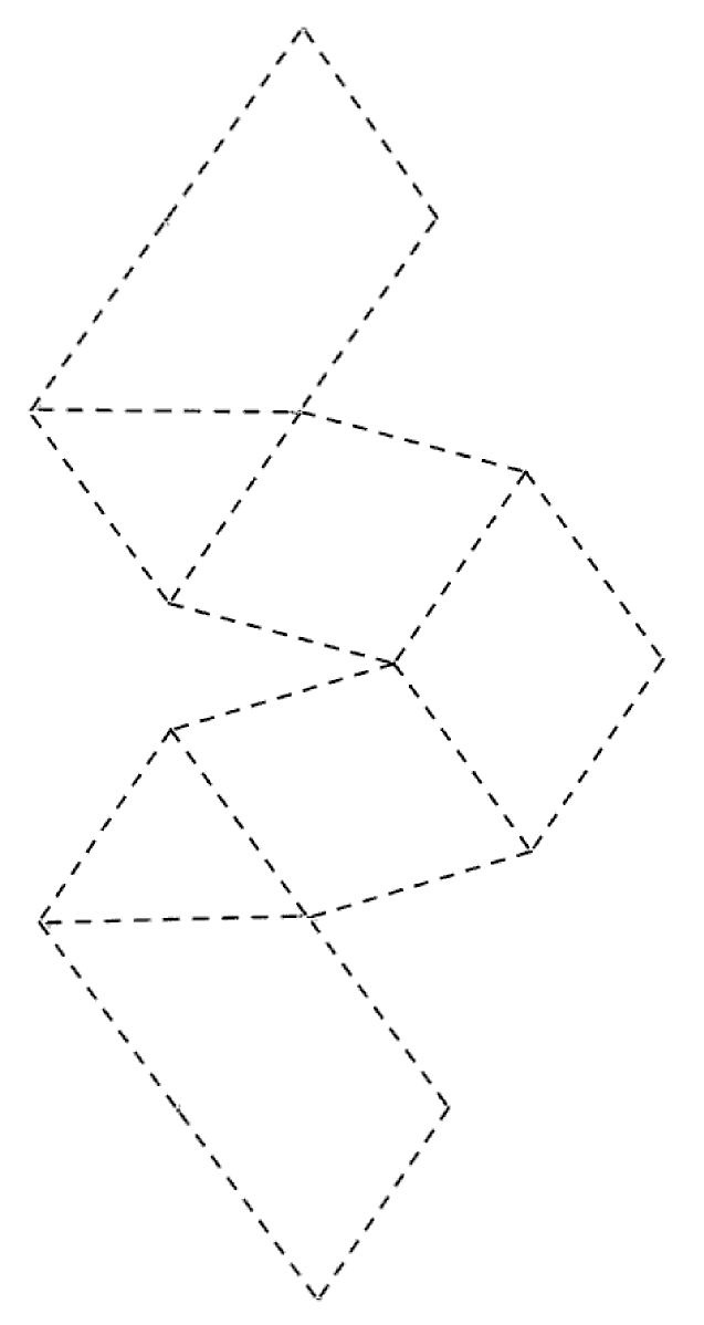
Figure 38: The $T^{6}/\Delta_{12}$ fundamental domain described in section 5.3.

References

- [1] M. R. Douglas and S. Kachru, Flux compactification, Rev. Mod. Phys. 79 (2007) 733–796 [hep-th/0610102].
- [2] M. P. Hertzberg, S. Kachru, W. Taylor and M. Tegmark, Inflationary Constraints on Type IIA String Theory, JHEP 12 (2007) 095 [arXiv:0711.2512].
- [3] S. Dimopoulos, S. Kachru, J. McGreevy and J. G. Wacker, N-flation, hep-th/0507205.
- [4] T. W. Grimm, Axion Inflation in Type II String Theory, Phys. Rev. D77 (2008) 126007 [0710.3883].
- [5] B. Florea, S. Kachru, J. McGreevy and N. Saulina, Stringy instantons and quiver gauge theories, JHEP 05 (2007) 024 [hep-th/0610003].
- [6] R. Blumenhagen, S. Moster and E. Plauschinn, Moduli Stabilisation versus Chirality for MSSM like Type IIB Orientifolds, JHEP 01 (2008) 058 [0711.3389].
- [7] J. Shelton, W. Taylor and B. Wecht, Nongeometric flux compactifications, JHEP 10 (2005) 085 [hep-th/0508133].
- [8] E. Silverstein, Simple de Sitter Solutions, Phys. Rev. D77 (2008) 106006 [0712.1196].
- [9] A. Adams, M. Ernebjerg and J. M. Lapan, Linear models for flux vacua, hep-th/0611084.
- [10] A. Adams, Conformal field theory and the Reid conjecture, hep-th/0703048.
- [11] S. Hellerman, J. McGreevy and B. Williams, Geometric constructions of nongeometric string theories, JHEP 01 (2004) 024 [hep-th/0208174].
- [12] B. R. Greene, A. D. Shapere, C. Vafa and S.-T. Yau, Stringy cosmic strings and noncompact Calabi-Yau manifolds, Nucl. Phys. B337 (1990) 1.
- [13] C. Vafa, Evidence for F-theory, Nucl. Phys. B469 (1996) 403–418 [hep-th/9602022].
- [14] A. Strominger, S.-T. Yau and E. Zaslow, Mirror symmetry is T-duality, Nucl. Phys. B479 (1996) 243–259 [hep-th/9606040].
- [15] K. Dasgupta and S. Mukhi, F-theory at constant coupling, Phys. Lett. B385 (1996) 125–131 [hep-th/9606044].
- [16] M. Gross and P. M. H. Wilson, Large complex structure limits of K3 surfaces, J. Differential Geom. 55 (2000) 475–546 [math.DG/0008018].
- [17] T. H. Buscher, A Symmetry of the String Background Field Equations, Phys. Lett. B194 (1987) 59.
- [18] T. H. Buscher, Path Integral Derivation of Quantum Duality in Nonlinear Sigma Models, Phys. Lett. B201 (1988) 466.
- [19] J. Loftin, S.-T. Yau and E. Zaslow, Affine Manifolds, SYZ Geometry, and the Y Vertex, math/0405061.
- [20] M. R. Gaberdiel and B. Zwiebach, Exceptional groups from open strings, Nucl. Phys. B518 (1998) 151–172 [hep-th/9709013].
- [21] M. Bershadsky et. al., Geometric singularities and enhanced gauge symmetries, Nucl. Phys. B481 (1996) 215–252 [hep-th/9605200].
- [22] M. Gross, Topological mirror symmetry, math/9909015.
- [23] A. Tomasiello, Topological mirror symmetry with fluxes, JHEP 06 (2005) 067 [hep-th/0502148].
- [24] W.-D. Ruan, Lagrangian torus fibration of quintic Calabi-Yau hypersurfaces I: Fermat quintic case, math/9904012.
- [25] D. Joyce, Singularities of special Lagrangian fibrations and the SYZ conjecture, math/0011179.
- [26] A. Sen, String network, JHEP 03 (1998) 005 [hep-th/9711130].
- [27] W. M. Fairbairn, T. Fulton and W. H. Klink, Finite and Disconnected Subgroups of and their Application to the Elementary-Particle Spectrum, Journal of Mathematical Physics 5 (July, 1964) 1038–1051.
- [28] C. M. Hull and P. K. Townsend, Unity of superstring dualities, Nucl. Phys. B438 (1995) 109–137 [hep-th/9410167].
- [29] A. Kumar and C. Vafa, U-manifolds, Phys. Lett. B396 (1997) 85–90 [hep-th/9611007].
- [30] N. Kaloper and R. C. Myers, The O(dd) story of massive supergravity, JHEP 05 (1999) 010 [hep-th/9901045].
- [31] N. Hitchin, Generalized Calabi-Yau manifolds, Quart. J. Math. Oxford Ser. 54 (2003) 281–308 [math/0209099].
- [32] M. Gualtieri, Generalized complex geometry, math/0401221.
- [33] M. Grana, R. Minasian, M. Petrini and A. Tomasiello, Supersymmetric backgrounds from generalized Calabi-Yau manifolds, JHEP 08 (2004) 046 [hep-th/0406137].
- [34] S. Kachru, M. B. Schulz, P. K. Tripathy and S. P. Trivedi, New supersymmetric string compactifications, JHEP 03 (2003) 061 [hep-th/0211182].
- [35] S. Gurrieri, J. Louis, A. Micu and D. Waldram, Mirror symmetry in generalized Calabi-Yau compactifications, Nucl. Phys. B654 (2003) 61–113 [hep-th/0211102].
- [36] M. Grana, R. Minasian, M. Petrini and A. Tomasiello, A scan for new N=1 vacua on twisted tori, JHEP 05 (2007) 031 [hep-th/0609124].
- [37] A. Lawrence, M. B. Schulz and B. Wecht, D-branes in nongeometric backgrounds, JHEP 07 (2006) 038 [hep-th/0602025].
- [38] A. Dabholkar and C. Hull, Generalised T-duality and non-geometric backgrounds, JHEP 05 (2006) 009 [hep-th/0512005].
- [39] C. M. Hull, A geometry for non-geometric string backgrounds, JHEP 10 (2005) 065 [hep-th/0406102].
- [40] A. Flournoy, B. Wecht and B. Williams, Constructing nongeometric vacua in string theory, Nucl. Phys. B706 (2005) 127–149 [hep-th/0404217].
- [41] C. M. Hull, Doubled geometry and T-folds, JHEP 07 (2007) 080 [hep-th/0605149].
- [42] J. Shelton, W. Taylor and B. Wecht, Generalized flux vacua, JHEP 02 (2007) 095 [hep-th/0607015].
- [43] K. Becker, M. Becker, C. Vafa and J. Walcher, Moduli stabilization in non-geometric backgrounds, Nucl. Phys. B770 (2007) 1–46 [hep-th/0611001].
- [44] J. Maharana and J. H. Schwarz, Noncompact symmetries in string theory, Nucl. Phys. B390 (1993) 3–32 [hep-th/9207016].
- [45] D. Brace, B. Morariu and B. Zumino, T-duality and Ramond-Ramond backgrounds in the matrix model, Nucl. Phys. B549 (1999) 181–193 [hep-th/9811213].
- [46] A. S. Schwarz, Morita equivalence and duality, Nucl. Phys. B534 (1998) 720–738 [hep-th/9805034].
- [47] D. Brace, B. Morariu and B. Zumino, Dualities of the matrix model from T-duality of the Type II string, Nucl. Phys. B545 (1999) 192–216 [hep-th/9810099].
- [48] E. Cremmer and B. Julia, The supergravity, Nucl. Phys. B159 (1979) 141.
- [49] E. Sezgin and A. Salam, Maximal extended supergravity theory in seven-dimensions, Phys. Lett. B118 (1982) 359.
- [50] E. Cremmer, B. Julia, H. Lu and C. N. Pope, Dualisation of dualities. I, Nucl. Phys. B523 (1998) 73–144 [hep-th/9710119].
- [51] S. Gukov, S.-T. Yau and E. Zaslow, Duality and fibrations on manifolds, hep-th/0203217.
- [52] K. S. Narain, M. H. Sarmadi and C. Vafa, Asymmetric orbifolds, Nucl. Phys. B288 (1987) 551.
- [53] M. T. Mueller and E. Witten, Twisting toroidally compactified heterotic strings with enlarged symmetry groups, Phys. Lett. B182 (1986) 28.
- [54] M. Dine and E. Silverstein, New M-theory backgrounds with frozen moduli, hep-th/9712166.
- [55] A. Dabholkar and J. A. Harvey, String islands, JHEP 02 (1999) 006 [hep-th/9809122].
- [56] R. Blumenhagen, L. Gorlich, B. Kors and D. Lust, Asymmetric orbifolds, noncommutative geometry and type I string vacua, Nucl. Phys. B582 (2000) 44–64 [hep-th/0003024].
- [57] M. R. Gaberdiel and S. Schafer-Nameki, D-branes in an asymmetric orbifold, Nucl. Phys. B654 (2003) 177–196 [hep-th/0210137].
- [58] K. Aoki, E. D’Hoker and D. H. Phong, On the construction of asymmetric orbifold models, Nucl. Phys. B695 (2004) 132–168 [hep-th/0402134].
- [59] Z. Kakushadze and S. H. H. Tye, Asymmetric orbifolds and grand unification, Phys. Rev. D54 (1996) 7520–7544 [hep-th/9607138].
- [60] C. Vafa, Modular Invariance and Discrete Torsion on Orbifolds, Nucl. Phys. B273 (1986) 592.
- [61] S. Hellerman and J. Walcher, Worldsheet CFTs for flat monodrofolds, hep-th/0604191.
- [62] D. S. Freed and C. Vafa, Global anomalies on orbifolds, Commun. Math. Phys. 110 (1987) 349.
- [63] D. D. Joyce, Compact Riemannian 7-manifolds with holonomy . I, J. Diff. Geom. 43 (1996) 291–328.
- [64] D. D. Joyce, Compact Riemannian 7-manifolds with holonomy . II, J. Diff. Geom. 43 (1996) 329–375.
- [65] D. D. Joyce, Compact manifolds with special holonomy, Oxford University Press (2000).
- [66] C. Vafa and E. Witten, On orbifolds with discrete torsion, J. Geom. Phys. 15 (1995) 189–214 [hep-th/9409188].
- [67] J.-H. Lee and N. C. Leung, Geometric structures on and Spin(7)-manifolds, math/0202045.
- [68] C. Vafa and E. Witten, Dual string pairs with N=1 and N=2 supersymmetry in four dimensions, Nucl. Phys. Proc. Suppl. 46 (1996) 225–247 [hep-th/9507050].
- [69] A. Sen, Duality and Orbifolds, Nucl. Phys. B474 (1996) 361–378 [hep-th/9604070].
- [70] M. R. Gaberdiel and P. Kaste, Generalised discrete torsion and mirror symmetry for manifolds, JHEP 08 (2004) 001 [hep-th/0401125].
- [71] B. R. Greene, C. I. Lazaroiu and M. Raugas, D-branes on nonabelian threefold quotient singularities, Nucl. Phys. B553 (1999) 711–749 [hep-th/9811201].
- [72] D. Berenstein, V. Jejjala and R. G. Leigh, D-branes on singularities: New quivers from old, Phys. Rev. D64 (2001) 046011 [hep-th/0012050].
- [73] A. Hanany and Y.-H. He, Non-Abelian finite gauge theories, JHEP 02 (1999) 013 [hep-th/9811183].
- [74] B. Feng, A. Hanany, Y.-H. He and N. Prezas, Discrete torsion, non-Abelian orbifolds and the Schur multiplier, JHEP 01 (2001) 033 [hep-th/0010023].
- [75] A. Dabholkar and J. Park, Strings on Orientifolds, Nucl. Phys. B477 (1996) 701–714 [hep-th/9604178].
- [76] M. Gutperle, Non-BPS D-branes and enhanced symmetry in an asymmetric orbifold, JHEP 08 (2000) 036 [hep-th/0007126].
- [77] S. Hellerman, New type II string theories with sixteen supercharges, hep-th/0512045.
- [78] O. Aharony, Z. Komargodski and A. Patir, The Moduli Space and M(atrix) Theory of 9d N=1 Backgrounds of M/String Theory, JHEP 05 (2007) 073 [hep-th/0702195].
- [79] P. Berglund, A. Klemm, P. Mayr and S. Theisen, On type IIB vacua with varying coupling constant, Nucl. Phys. B558 (1999) 178–204 [hep-th/9805189].
- [80] M. Bershadsky, T. Pantev and V. Sadov, F-theory with quantized fluxes, Adv. Theor. Math. Phys. 3 (1999) 727–773 [hep-th/9805056].
- [81] S. Chaudhuri, G. Hockney and J. D. Lykken, Maximally supersymmetric string theories in , Phys. Rev. Lett. 75 (1995) 2264–2267 [hep-th/9505054].
- [82] S. Chaudhuri and J. Polchinski, Moduli space of CHL strings, Phys. Rev. D52 (1995) 7168–7173 [hep-th/9506048].
- [83] E. Witten, String theory dynamics in various dimensions, Nucl. Phys. B443 (1995) 85–126 [hep-th/9503124].
- [84] A. Sen, M-Theory on , Phys. Rev. D53 (1996) 6725–6729 [hep-th/9602010].
- [85] E. Witten, Phases of N = 2 theories in two dimensions, Nucl. Phys. B403 (1993) 159–222 [hep-th/9301042].
- [86] D. Morrison, unpublished.
- [87] C. M. Hull, Gravitational duality, branes and charges, Nucl. Phys. B509 (1998) 216–251 [hep-th/9705162].
- [88] J. Polchinski, String theory. Vol. 2: Superstring theory and beyond, Cambridge University Press (1998).
- [89] C. Saclioglu, Generalization of Weierstrassian elliptic functions to , J. Phys. A29 (1996) L17–L22 [hep-th/9506060].
- [90] S. Hellerman, unpublished.
- [91] G. W. Gibbons and P. J. Ruback, The Hidden Symmetries of Multicenter Metrics, Commun. Math. Phys. 115 (1988) 267.
- [92] H. Ooguri and C. Vafa, Summing up D-instantons, Phys. Rev. Lett. 77 (1996) 3296–3298 [hep-th/9608079].
- [93] A. Hanany and E. Witten, Type IIB superstrings, BPS monopoles, and three-dimensional gauge dynamics, Nucl. Phys. B492 (1997) 152–190 [hep-th/9611230].
- [94] S. Elitzur, A. Giveon and D. Kutasov, Branes and N = 1 duality in string theory, Phys. Lett. B400 (1997) 269–274 [hep-th/9702014].
- [95] N. Seiberg, Electric - magnetic duality in supersymmetric nonAbelian gauge theories, Nucl. Phys. B435 (1995) 129–146 [hep-th/9411149].
- [96] S. H. Katz, A. Klemm and C. Vafa, Geometric engineering of quantum field theories, Nucl. Phys. B497 (1997) 173–195 [hep-th/9609239].
- [97] H. Ooguri and C. Vafa, Geometry of N = 1 dualities in four dimensions, Nucl. Phys. B500 (1997) 62–74 [hep-th/9702180].
- [98] E. Witten, Solutions of four-dimensional field theories via M- theory, Nucl. Phys. B500 (1997) 3–42 [hep-th/9703166].
- [99] S. Elitzur, A. Giveon, D. Kutasov, E. Rabinovici and A. Schwimmer, Brane dynamics and N = 1 supersymmetric gauge theory, Nucl. Phys. B505 (1997) 202–250 [hep-th/9704104].
- [100] B. Feng, A. Hanany and Y.-H. He, D-brane gauge theories from toric singularities and toric duality, Nucl. Phys. B595 (2001) 165–200 [hep-th/0003085].
- [101] I. R. Klebanov and M. J. Strassler, Supergravity and a confining gauge theory: Duality cascades and chiSB-resolution of naked singularities, JHEP 08 (2000) 052 [hep-th/0007191].
- [102] F. Cachazo, B. Fiol, K. A. Intriligator, S. Katz and C. Vafa, A geometric unification of dualities, Nucl. Phys. B628 (2002) 3–78 [hep-th/0110028].
- [103] C. E. Beasley and M. R. Plesser, Toric duality is Seiberg duality, JHEP 12 (2001) 001 [hep-th/0109053].
- [104] B. Feng, A. Hanany, Y.-H. He and A. M. Uranga, Toric duality as Seiberg duality and brane diamonds, JHEP 12 (2001) 035 [hep-th/0109063].
- [105] D. Berenstein and M. R. Douglas, Seiberg duality for quiver gauge theories, hep-th/0207027.
- [106] S. Franco, A. Hanany, K. D. Kennaway, D. Vegh and B. Wecht, Brane dimers and quiver gauge theories, JHEP 01 (2006) 096 [hep-th/0504110].
- [107] A. Hanany and D. Vegh, Quivers, tilings, branes and rhombi, JHEP 10 (2007) 029 [hep-th/0511063].
- [108] G. ’t Hooft, A locally finite model for gravity, 0804.0328.
- [109] E. Witten, Five-branes and M-theory on an orbifold, Nucl. Phys. B463 (1996) 383–397 [hep-th/9512219].
- [110] K. Dasgupta and S. Mukhi, Orbifolds of M-theory, Nucl. Phys. B465 (1996) 399–412 [hep-th/9512196].
- [111] A. Sen, A note on enhanced gauge symmetries in M- and string theory, JHEP 09 (1997) 001 [hep-th/9707123].
- [112] S. Kachru and J. McGreevy, M-theory on manifolds of holonomy and Type IIA orientifolds, JHEP 06 (2001) 027 [hep-th/0103223].
- [113] A. Dabholkar, Lectures on orientifolds and duality, hep-th/9804208.
- [114] M. R. Douglas, D-branes and discrete torsion, hep-th/9807235.