Beyond the frame rate: Measuring high-frequency fluctuations with light intensity modulation

Wesley P. Wong^∗ and Ken Halvorsen^†

The Rowland Institute at Harvard, Harvard University, Cambridge, Massachusetts 02142, USA
^∗Corresponding author: wong@rowland.harvard.edu   ^†Both authors contributed equally
Journal-ref: Optics Letters 34(3), 277–279 (2009)

Abstract

Power spectral density measurements of any sampled signal are typically restricted by both acquisition rate and frequency response limitations of instruments, which can be particularly prohibitive for video-based measurements. We have developed a new method called Intensity Modulation Spectral Analysis (IMSA) that circumvents these limitations, dramatically extending the effective detection bandwidth. We demonstrate this by video-tracking an optically-trapped microsphere while oscillating an LED illumination source. This approach allows us to quantify fluctuations of the microsphere at frequencies over 10 times higher than the Nyquist frequency, mimicking a significantly higher frame rate.

OCIS codes:  170.4520, 110.4155, 120.4820

Measuring the power spectral density (PSD) is a useful way to characterize fluctuations and noise for a diverse range of physical processes. Optical measurements of the PSD have been used to study single molecule dynamics [1], bacterial chemotaxis and motion [2, 3], quantum dot blinking [4] and microrheology [5, 6], and to calibrate optical traps [7]. Unfortunately, limited acquisition rate and detector frequency response restrict PSD measurements in frequency space, which is especially detrimental to video applications. Notably, the highest frequency that can be sampled directly, with few exceptions [8, 9, 10, 11], is half the acquisition rate, or Nyquist frequency.

We have developed a method called Intensity Modulation Spectral Analysis (IMSA), which overcomes these limitations in a simple and economical way. By simply oscillating the light intensity of an optical signal prior to detection, the PSD at the oscillation frequency can be determined from the measured variance, even if that frequency is above the acquisition rate. This is similar in spirit to signal processing methods that can spectrally shift a signal (e.g. heterodyne detection, lock-in techniques), or extract high-frequency information folded down via aliasing (e.g. undersampling [11, 12]). Practically, IMSA can dramatically extend the frequency range of an existing measurement device, allowing, for example, an inexpensive camera to be used in place of a significantly more expensive one. Here we present the framework for IMSA and an experimental demonstration using an optically-trapped microsphere, in which modulating the brightness of an LED allows PSD measurement well beyond the Nyquist frequency and camera frame rate.

IMSA: Concept and foundations

Physical acquisition systems do not make instantaneous measurements when sampling a signal, but rather collect data over finite integration times. Consider a stationary random trajectory $X(t)$. The measured trajectory $X_{m}(t)$ can be expressed as a convolution of the true trajectory and an impulse response $H(t)$:

$$X_{m}(t)=(X\ast H)(t)\equiv\int X(t^{\prime})H(t-t^{\prime})\mathrm{d}{t^{\prime}}\;$$ (1)

Then the measured power spectrum $P_{m}(\omega)$ differs from $P(\omega)$, the true power spectrum of $X$, according to the relation $P_{m}(\omega)=P(\omega)|\tilde{H}(\omega)|^{2}$, and the total measured variance is the integral of $P_{m}(\omega)$ over all frequencies:

$$\text{var}[X_{m}]=\frac{1}{2\pi}\int P(\omega)\left|\tilde{H}(\omega)\right|^{2}\mathrm{d}{\omega}\;$$ (2)

where the tilde designates the Fourier transform, $\tilde{X}(\omega)=\int X(t)\exp(-i\omega t)\mathrm{d}{t}\;$. Integrals are taken from $-\infty$ to $+\infty$ unless otherwise specified.

In the simplest case, the measured quantity $X_{m}$ is the unweighted time average of the true value $X$ over the integration time $W$, i.e. the impulse response is a rectangular function:

$$H_{0}(t)=\left\{\begin{array}[]{cl}\frac{1}{W}&-W/2<t\leq W/2\\ 0&\text{elsewhere}\end{array}\right.$$ (3)

Correspondingly, the measured power spectrum is the original power spectrum multiplied by:

$$\left|\tilde{H}_{0}(\omega)\right|^{2}=\left({\frac{\sin(\omega W/2)}{\omega W/2}}\right)^{2}$$ (4)

This simple case of a rectangular impulse response is a good model for video-imaging acquisition systems, where $W$ is the exposure time. This averaging leads to the common problem of video image blur, which not only adds errors in the position of tracked objects, but also causes systematic biases when quantifying fluctuations [13, 14, 15, 10]. As we have previously demonstrated [10], by measuring the variance for different exposure times $W$ and fitting to equation 2, the power spectrum can be characterized above the acquisition rate of the detection system. However, this approach requires that the functional form of the power spectrum is known a priori.

Interestingly, by oscillating the intensity of a source signal (e.g. light in the case of video imaging) and measuring the variance of the resulting signal, the power spectrum can be reconstructed without prior knowledge. This is the fundamental idea behind IMSA.

During detection, the finite integration time $W$ causes the true power spectrum to be multiplied by the low-pass filter $|\tilde{H}_{0}(\omega)|^{2}$ (equation 4). As $W$ becomes longer, $|\tilde{H}_{0}(\omega)|^{2}$ approaches an unnormalized delta function, i.e. $|\tilde{H}_{0}(\omega)|^{2}\rightarrow\alpha\delta(\omega)$. Multiplying the rectangular impulse response by a complex exponential shifts this delta function, i.e. if $H(t)=\exp(-i\omega^{\prime}t)H_{0}(t)$, then $|\tilde{H}(\omega)|^{2}\rightarrow\alpha\delta(\omega-\omega^{\prime})$. From equation 2 we see that the variance approaches $\alpha P(\omega^{\prime})/2\pi$. Thus, as demonstrated in this simple example, the power spectrum can be sampled by shifting the filter to any frequency of interest $\omega^{\prime}$ and measuring the variance.

Practically, we use the real-valued impulse response

$$H(t)=L(t)H_{0}(t)/N$$ (5)

where $L(t)\equiv\sin(\omega^{\prime}t+\phi)+B$ and $N$ is a normalization factor (see Fig. 1). We set $N=\int L(t)H_{0}(t)\mathrm{d}{t}\;$ so that the convolution represents a time-averaged signal weighted by the source intensity modulation $L(t)$, and let $B\geq 0$; the parameters ($W$, $B$) should be chosen such that $N\neq 0$. Note that $N=B$ whenever $\phi$ (the phase-shift between modulation and sampling) is an integer multiple of $2\pi$, or whenever there are an integer number of oscillations within each exposure window.

By substituting $\tilde{H}(\omega)$ (the Fourier transform of equation 5) into equation 2, and noting that $P(-\omega)=P(\omega)$ for a real-valued wide-sense stationary process, we obtain for the measured variance:

$$\text{var}[X_{m}]=\frac{1}{4\pi N^{2}}\int P(\omega)\left|\tilde{H}_{0}(\omega-\omega^{\prime})\right|^{2}\mathrm{d}{\omega}\;$$ (t1)

$$\quad+\frac{B^{2}}{2\pi N^{2}}\int P(\omega)\left|\tilde{H}_{0}(\omega)\right|^{2}\mathrm{d}{\omega}\;$$ (t2)

$$\quad+\frac{B\sin(\phi)}{\pi N^{2}}\int P(\omega)\tilde{H}_{0}(\omega)\tilde{H}_{0}(\omega-\omega^{\prime})\mathrm{d}{\omega}\;$$ (t3)

$$\quad-\frac{\cos(2\phi)}{4\pi N^{2}}\int P(\omega)\tilde{H}_{0}(\omega+\omega^{\prime})\tilde{H}_{0}(\omega-\omega^{\prime})\mathrm{d}{\omega}\;$$ (t4)

This key equation can be used to determine the power spectrum from the measured variance, since term t1 approaches $P(\omega^{\prime})/2WN^{2}$ as $W$ gets longer (see endnote [16] and Fig. 1), while terms t3 and t4 become small and term t2 can be measured directly. Additionally, proper phase selection can completely eliminate t3 and t4.

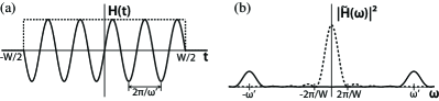
Fig. 1: Graphical representation of IMSA showing (a) unnormalized impulse responses $H(t)=L(t)H_{0}(t)$ for $\phi=0$ and $B=0$ (solid line, see equation 5) and $H(t)=H_{0}(t)$ (dotted line, see equation 3), and (b) the squared magnitude of their Fourier transforms, which filter $P(\omega)$ in terms t1 and t2 of equation LABEL:eq:measuredvarfullexpressioneven.

IMSA Usage

To determine the power spectral density of a signal at the frequency of interest $\omega^{\prime}$, the signal should be convolved with $L(t)H_{0}(t)/N$ (equation 5) by modulating its intensity, and then its variance should be measured. Writing the measured variance as $\text{var}[X_{m}](\omega^{\prime})$, the PSD is given by the following formulas:
When $B=0$,

$$P(\omega^{\prime})=2WN^{2}\text{var}[X_{m}](\omega^{\prime})$$ (7)

provided $\phi=\pi/4+m\pi/2$, where $m$ is an integer.
When $B\neq 0$,

$$P(\omega^{\prime})=2WB^{2}\left(\text{var}[X_{m}](\omega^{\prime})-\text{var}[X_{m}](0)\right)$$ (8)

provided that the exposure time $W$ is chosen such that $W=n2\pi/\omega^{\prime}$ where $n$ is a natural number, and $\phi$ is chosen according to (see endnote [17]):

$$\phi=(-1)^{n}\sin^{-1}\left(\sqrt{B^{2}+1/2}-B\right)$$ (9)

On a practical note, terms t3 and t4 are small when $W\gg 1/\omega^{\prime}$ (i.e. there are many oscillation cycles within each exposure window). If both cross-terms t3 and t4 are negligible, the selection of $\phi$ is irrelevant. In fact, oscillations may not even have to be synchronized to the acquisition device to make a good IMSA measurement—simply multiplying the input signal by $L(t)$ prior to detection can yield acceptable results.

The error in $P(\omega^{\prime})$ is governed primarily by the error in the variance (e.g. for $N$ samples the relative statistical standard error is $\sqrt{(}2/N)$, barring instrumental error [10]). The resolution in $\omega^{\prime}$ is given by the width of $|\tilde{H}_{0}(\omega)|^{2}$ (see Fig. 1), which is approximately $\pi/W$ in each direction (77% of the area under the curve).

Experimental Demonstration

To demonstrate IMSA experimentally, we measured the power spectrum of an optically trapped polystyrene microsphere (2.5 um, Corpuscular) using a machine vision camera (GE680, Prosilica) and an LED (MRMLED, Thorlabs) with intensity modulation capable of up to 300kHz (custom current source, Rowland Institute electronics lab). Details of the particle tracking have been discussed previously for a functionally identical setup, where it was demonstrated that the system is well-described by equation 3 [10]. The light intensity was sinusoidally modulated (as in equation 5) with $B=0.5$ and $\phi$ determined from equation 9, and the integration time of the camera was $W=2.5$ ms. Modulated light at 5 different frequencies $\omega^{\prime}$ was interspersed with DC light on a frame by frame basis. Each of the 10 variances was calculated and each PSD data point was calculated according to equation 8, where the mean of the two neighboring DC frames was used as $\text{var}[X_{m}](0)$ for each of the 5 measurements. Data was collected for two beads at different laser powers. The spring constant and friction factor for each bead was measured using the blur-corrected power spectrum method [10]. The IMSA measured values, which have no free fitting parameters, are in excellent agreement with the expected power spectra (Fig. 2).

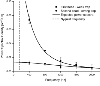
Fig. 2: Measurement of the power spectrum using IMSA for two trapped beads with different spring constants (data points). The expected power spectra are superimposed (solid lines), showing good agreement well beyond the Nyquist frequency (vertical dashed line). Error bars represent statistical error.

Concluding Discussion

As we have shown, IMSA provides a unique and practical way for measuring the PSD of a signal, which overcomes acquisition rate and frequency response limitations of instruments. While especially beneficial to video imaging applications (due to the almost negligible cost of implementation compared with the expense of fast video cameras), IMSA is a general method applicable to signals in which the time-averaged weighting can be controlled before sampling.

Owing to its potential to benefit a broad range of fields and its flexibility of implementation (see endnote [18]), we expect that IMSA will become a common laboratory method for measuring power spectra. Microrheology measurements [19, 6] can take immediate advantage of the up to $\sim 10000$ fold increase in frequency range over standard video imaging, without losing the ability to track multiple targets. Widely used fluorescence-imaging techniques [20] stand to benefit as well, with IMSA enabling measurements at frequencies which are currently impossible by any other method owing to light limitations.

The dramatic increase in frequency range enabled by IMSA can be used to push the envelope of high frequency measurement and to realize significant cost savings in instrumentation. Using an inexpensive LED illuminator, we transformed a standard video camera into a spectrum analyzer with a frequency range of up to $\sim 300$ kHz.

References

- [1] L. Oddershede, J. K. Dreyer, S. Grego, S. Brown, and K. Berg-Sørensen, “The Motion of a Single Molecule, the -Receptor, in the Bacterial Outer Membrane,” Biophys. J. 83, 3152–3161 (2002).
- [2] C. V. Gabel and H. C. Berg, “The speed of the flagellar rotary motor of Escherichia coli varies linearly with protonmotive force,” Proc. Natl. Acad. Sci. U.S.A. 100, 8748–8751 (2003).
- [3] E. Korobkova, T. Emonet, J. M. G. Vilar, T. S. Shimizu, and P. Cluzel, “From molecular noise to behavioural variability in a single bacterium,” Nature 428, 574–578 (2004).
- [4] M. Pelton, D. G. Grier, and P. Guyot-Sionnest, “Characterizing quantum-dot blinking using noise power spectra,” Appl. Phys. Lett. 85, 819 (2004).
- [5] F. Gittes, B. Schnurr, P. D. Olmsted, F. C. MacKintosh, and C. F. Schmidt, “Microscopic Viscoelasticity: Shear Moduli of Soft Materials Determined from Thermal Fluctuations,” Phys. Rev. Lett. 79, 3286–3289 (1997).
- [6] M. T. Valentine, P. D. Kaplan, D. Thota, J. C. Crocker, T. Gisler, R. K. Prud’homme, M. Beck, and D. A. Weitz, “Investigating the microenvironments of inhomogeneous soft materials with multiple particle tracking,” Phys. Rev. E 64, 61506 (2001).
- [7] K. Svoboda and S. M. Block, “Biological Applications of Optical Forces,” Annu. Rev. Biophys. Biomol. Struct. 23, 247–285 (1994).
- [8] F. R. Verdun, T. L. Ricca, and A. G. Marshall, “Beating the Nyquist Limit by Means of Interleaved Alternated Delay Sampling: Extension of Lower Mass Limit in Direct-Mode Fourier Transform Ion Cyclotron Resonance Mass Spectrometry,” Appl. Spectros. 42, 199–203 (1988).
- [9] M. H. El-Shafey, “Beating the nyquist limit by utilizing samples of filtered sinisoids,” in “Proc. ICEEC’04,” (Cairo, Egypt, 2004), pp. 210–213.
- [10] W. P. Wong and K. Halvorsen, “The effect of integration time on fluctuation measurements: calibrating an optical trap in the presence of motion blur,” Opt. Express 14, 12517–12531 (2006).
- [11] C. Donciu, C. Temneanu, and R. Ciobanu, “Breaking nyquist criteria using alias frequencies interpretation,” in “Proc. IEEE Int. Conf. VECIMS 2005,” (Taormina, Sicily, Italy, 2005), pp. 50–53.
- [12] R. G. Vaughan, N. L. Scott, and D. R. White, “The theory of bandpass sampling,” IEEE Trans. Sig. Proc. 39, 1973–1984 (1991).
- [13] R. Yasuda, H. Miyata, and K. Kinosita, Jr, “Direct Measurement of the Torsional Rigidity of Single Actin Filaments,” J. Mol. Biol. 263, 227–236 (1996).
- [14] T. Savin and P. S. Doyle, “Static and Dynamic Errors in Particle Tracking Microrheology,” Biophys. J. 88, 623–638 (2005).
- [15] T. Savin and P. S. Doyle, “Role of a finite exposure time on measuring an elastic modulus using microrheology,” Phys. Rev. E 71, 41106 (2005).
- [16] Noting that .
- [17] Determination of to eliminate terms t3 and t4 can be done by calculating , setting the sum of the -dependent terms to zero and solving for the specific case where .
- [18] For example, measurement sensitivity can be improved by removing the DC offset (i.e. set B=0). For video imaging, this can be accomplished by simulating positive and negative light (e.g. by using two colors or polarizations), or for low light applications, by properly synchronizing two camera frames to each illumination cycle. At the sensor level, IMSA can be implemented by using a camera capable of modulating the incoming signal [21, 22, 23], or by having two collection wells for each pixel to simulate positive and negative light.
- [19] J. C. Crocker and D. G. Grier, “Methods of Digital Video Microscopy for Colloidal Studies,” J. Colloid Interface Sci. 179, 298–310 (1996).
- [20] E. Toprak and P. R. Selvin, “New fluorescent tools for watching nanometer-scale conformational changes of single molecules,” Annu. Rev. Biophys. Biomol. Struct. 36, 349–369 (2007).
- [21] A. C. Mitchell, J. E. Wall, J. G. Murray, and C. G. Morgan, “Direct modulation of the effective sensitivity of a CCD detector: a new approach to time-resolved fluorescence imaging.” J. Microsc. 206, 225–232 (2002).
- [22] P. R. Dmochowski, B. R. Hayes-Gill, M. Clark, J. A. Crowe, M. G. Somekh, and S. P. Morgan, “Camera pixel for coherent detection of modulated light,” Electron. Lett. 40, 1403–1404 (2004).
- [23] D. Van Nieuwenhove, W. van der Tempel, R. Grootjans, J. Stiens, and M. Kuijk, “Photonic Demodulator With Sensitivity Control,” IEEE Sens. J. 7, 317–318 (2007).
Acknowledgments
Thanks to M. M. Burns, W. Hill, A. M. Turner, and M. M. Forbes for helpful conversations, and C. Stokes for the LED current source. Funding was provided by the Rowland Junior Fellows program.