MEASURING DISLOCATION DENSITY IN ALUMINUM WITH RESONANT ULTRASOUND SPECTROSCOPY

Abstract

Dislocations in a material will, when present in enough numbers, change the speed of propagation of elastic waves. Consequently, two material samples, differing only in dislocation density, will have different elastic constants, a quantity that can be measured using Resonant Ultrasound Spectroscopy. Measurements of this effect on aluminum samples are reported. They compare well with the predictions of the theory.

Keywords: Resonant Ultrasound Spectroscopy, Dislocation density.

I Introduction

A series of papers by Maurel et al. [2004a; 2004b; 2005a; 2005b; 2006; 2007a; 2007b] have constructed a detailed theory of the interaction of elastic waves with dislocations in elastic, homogeneous and isotropic, solids. This has been done both in two and three dimensions. Dislocations have ben considered both in isolation as well as in large numbers. In the latter case, generalization of the Granato & Lücke [1956a; 1956b; 1966] theory has emerged with results for change in wave propagation velocity and attenuation length that clearly distinguish between longitudinal (acoustic) and transverse (shear) polarizations. These results are in satisfactory agreement with laboratory measurements of acoustic attenuation using Resonant Ultrasound Spectroscopy—RUS [Ledbetter & Fortunko, 1995; Ogi et al., 1999; 2004; Ohtani et al., 2005]. The case of an isolated dislocation in a half-space has also been studied, as well as the case of low angle grain boundaries mimicked as dislocation arrays.

A natural development of the above ideas and results is to ask whether RUS can be turned into a practical tool to measure dislocation densities in materials. In order to do this, it is necessary to validate whatever results are obtained using RUS with time-tested, but more involved, High Resolution Transmission Electron Microscopy [Williams & Carter, 2004; Arakawa et al., 2006; Robertson et al., 2008]. A preliminary step towards that aim is to perform RUS measurements on a number of samples of a given material, one as received from the provider, and the others after cold rolling, or annealing, so as to have significantly different dislocation densities. This paper reports a simplified form of the theory, as well as the first such measurements, using aluminum.

II Effective velocity of elastic waves in a dislocation-filled medium

We study an homogeneous, isotropic, three-dimensional, infinite elastic medium of density $\rho$, whose state is described by a vector field $\vec{u}(\vec{x},t)$, the displacement $\vec{u}$ at time $t$ of a point whose equilibrium position is at $\vec{x}$. In the absence of dislocations, the displacement $\vec{u}$ obeys the wave equation

$$\rho\frac{\partial^{2}u_{i}}{\partial t^{2}}-c_{ijkl}\frac{\partial^{2}u_{k}}{\partial x_{j}\partial x_{l}}=0$$ (1)

with $c_{ijkl}=\lambda\delta_{ij}\delta_{kl}+\mu(\delta_{ik}\delta_{jl}+\delta_{il}\delta_{jk})$ the tensor of elastic constants, and $i,j,k,\dots=1,2,3$. A consequence of this equation is that the medium allows for the propagation of longitudinal (acoustic) and transverse (shear) waves with propagation velocity $c_{L}=\sqrt{(\lambda+2\mu)/\rho}$ and $c_{T}=\sqrt{\mu/\rho}$, respectively. Their ratio $\gamma=c_{L}/c_{T}>1$ is always greater than one.

Dislocations are modeled as one dimensional objects (“strings”, [Koehler, 1952; Granato & Lücke, 1956a,b]) $\vec{X}(s,t)$, where $s$ is a Lagrangean parameter that labels points along the line, and $t$ is time, of length $L$, pinned at the ends, whose equilibrium position is a straight line. They are characterized by a Burgers vector $\vec{b}$, perpendicular to the equilibrium line. Their unforced motion is described by a conventional vibrating string equation

$$m\frac{\partial^{2}X_{i}}{\partial t^{2}}+B\frac{\partial X_{i}}{\partial t}-\Gamma\frac{\partial^{2}X_{i}}{\partial s^{2}}=0$$ (2)

where the mass per unit length $m$ and line tension $\Gamma$ are given by [Lund, 1988]

$$m = \frac{\rho b^{2}}{4\pi}\left(1+\gamma^{-4}\right)\ln\left(\frac{\delta}{\delta_{0}}\right)$$

$$\Gamma = \frac{\rho b^{2}c_{T}^{2}}{4\pi}\left(1-\gamma^{-2}\right)\ln\left(\frac{\delta}{\delta_{0}}\right)$$ (3)

where $\delta$ and $\delta_{0}$ are external and internal cut-offs. The coefficient $B$ is a phenomenological term that describes the internal losses of the string due to, for example, interactions with phonons and electrons. We shall only consider glide motion, that is, motion parallel to the Burgers vector $\vec{b}$.

When elastic waves and dislocations interact, both Eqns. (1) and (2) acquire right hand side—source—terms, whose structure has been discussed in detail by Maurel et al. [2005a,b]. Elastic waves in the presence of $N$ dislocations are best described not in terms of particle displacement $\vec{u}$ but in terms of particle velocity $\vec{v}=\partial\vec{u}/\partial t$ and the wave equation (1) becomes

$$\rho\frac{\partial^{2}v_{i}}{\partial t^{2}}-c_{ijkl}\frac{\partial^{2}v_{k}}{\partial x_{j}\partial x_{l}}=s_{i}$$ (4)

where the source term $s_{i}$ is given by

$$s_{i}(\vec{x},t) = c_{ijkl}\epsilon_{mnk}\sum_{n=1}^{N}\int_{\cal L}ds\;\dot{X}_{m}^{n}(s,t)\tau_{n}b_{l}$$ (5)

$$\mbox{}\times\frac{\partial}{\partial x_{j}}\delta(\vec{x}-\vec{X}^{n}(s,t)).$$

where $\epsilon_{mnk}$ is the completely antisymmetric tensor of order three, and $\hat{\tau}$ is a unit tangent along the dislocation line. The string equation (2) is written for the component of motion along the glide direction, $X\equiv X_{k}t_{k}$ and, loaded by a Peach-Koehler [1950] force it becomes

$$m\ddot{X}(s,t)+B\dot{X}(s,t)-\Gamma X^{\prime\prime}(s,t)=\mu b\;{\mathsf{M}}_{lk}\partial_{l}u_{k}(\vec{X},t),$$ (6)

with ${\mathsf{M}}_{lk}\equiv t_{l}n_{k}+t_{k}n_{l}$ and $\hat{n}\equiv\hat{\tau}\times\hat{t}$ a unit binormal vector. Overdots mean time derivatives, and primes mean derivatives with respect to $s$.

At this point it becomes profitable to go to the frequency domain. The loaded string equation (6) can be solved in terms of normal modes, and the solution plugged into the right hand side of the wave equation (4). In the long wavelength limit, $\lambda\gg L$, and for small string displacements, the result of this operation is

$$-\rho\omega^{2}v_{i}-c_{ijkl}\frac{\partial^{2}v_{k}}{\partial x_{j}\partial x_{l}}=V_{ik}v_{k}$$ (7)

where

$$V_{ik}=\frac{8L}{\pi^{2}}\frac{(\mu b)^{2}}{m}\frac{S(\omega)}{\omega^{2}}\;\sum_{n=1}^{N}{\mathsf{M}}^{n}_{ij}\frac{\partial}{\partial x_{j}}\delta(\vec{x}-\vec{X}^{n}_{0})\;{\mathsf{M}}^{n}_{lk}{\frac{\partial}{\partial x_{l}}}$$ (8)

and

$$S(\omega)\simeq\frac{\omega^{2}}{\omega^{2}-\omega_{1}^{2}+i\omega B/m}.$$ (9)

with

$$\omega_{1}=\frac{\pi}{L}\sqrt{\frac{\Gamma}{m}}$$

the frequency of the fundamental mode of the string with fixed ends.

Maurel et al. [2005b] have provided two derivations of effective velocities for elastic waves described by Eqn. (8). Here we give a third, with a reasoning similar to the one used to study waves in plasmas [Stix, 1992]: The right-hand-side (8) is smoothed through the replacement of the discrete sum over dislocation segments by an integral over space with a continuous density $n(\vec{x})$ of dislocation segments, and the tensor ${\mathsf{M}}^{n}_{ij}{\mathsf{M}}^{n}_{lk}$ by its angular average, assuming all directions equally likely. The last operation can be found in Appendix C of Maurel et al. [2005b]. Eqn. (7) thus becomes, in the case of uniform dislocation density $n(\vec{x})=n$,

$$-\rho\omega^{2}v_{i}-c_{ijkl}\frac{\partial^{2}v_{k}}{\partial x_{j}\partial x_{l}}=$$ (10)

$$\frac{8}{\pi^{2}}\frac{(\mu b)^{2}}{m}\frac{S(\omega)}{\omega^{2}}\frac{nL}{15}(3\delta_{ik}\delta_{lj}+\delta_{il}\delta_{kj})\frac{\partial^{2}v_{k}}{\partial x_{j}\partial x_{l}}$$

In wave number space this is an equation

$${\cal O}_{ik}v_{k}=0$$ (11)

with

$${\cal O}_{ik} \equiv -\rho\omega^{2}\delta_{ik}+c_{ijkl}k_{j}k_{l}+\frac{8}{\pi^{2}}\frac{(\mu b)^{2}}{m}\frac{S(\omega)}{\omega^{2}}\frac{nL}{15}$$

$$\mbox{}\times(3\delta_{ik}\delta_{lj}+\delta_{il}\delta_{kj})k_{j}k_{l}.$$

The dispersion relation for the elastic waves in this averaged medium is given by the vanishing of the determinant of $\cal O$:

$$\det{\cal O}=0$$ (12)

For frequencies smaller than the fundamental frequency of the string, $\omega\ll\omega_{1}$, and small damping, $(\omega B/m)\ll\omega_{1}^{2}$, this leads to the following effective longitudinal $(v_{L})$ and transverse $(v_{T})$ phase velocities:

$$v_{L} = c_{L}\left(1-\frac{16}{15\pi^{4}}\frac{1}{\gamma^{2}}\frac{\mu b^{2}}{\Gamma}\;nL^{3}\right)$$ (13)

$$v_{T} = c_{T}\left(1-\frac{4}{5\pi^{4}}\frac{\mu b^{2}}{\Gamma}\;nL^{3}\right).$$ (14)

III RUS measurements

Parameter	Sample 1	Sample 2	Sample 3	Sample 4	Sample 5
Preparation	Annealed $400^{\circ}$C/10 hrs	Annealed $400^{\circ}$C/5 hrs	Original	Rolled at 33%	Rolled at 43%
$d_{1}$ [cm]	$1.701\pm 0.001$	$1.700\pm 0.001$	$1.7004\pm 0.0003$	$1.696\pm 0.001$	$1.7004\pm 0.0005$
$d_{2}$ [cm]	$1.0010\pm 0.0004$	$0.9992\pm 0.0004$	$0.9991\pm 0.0005$	$1.000\pm 0.001$	$1.0005\pm 0.0003$
$d_{3}$ [cm]	$5.002\pm 0.001$	$5.002\pm 0.001$	$5.000\pm 0.001$	$5.000\pm 0.001$	$5.001\pm 0.002$
$\rho$ [g/cm3]	$2.691\pm 0.002$	$2.692\pm 0.002$	$2.696\pm 0.002$	$2.692\pm 0.004$	$2.691\pm 0.002$
$C_{11}$ [$10^{11}$ Pa]	$0.868\pm 0.038$	$0.880\pm 0.023$	$0.884\pm 0.028$	$0.888\pm 0.026$	$0.883\pm 0.023$
$C_{44}$ [$10^{11}$ Pa]	$0.2680\pm 0.0017$	$0.2664\pm 0.0007$	$0.2661\pm 0.0008$	$0.2647\pm 0.0007$	$0.2643\pm 0.0007$
$v_{L}$ [m/s]	$5679\pm 124$	$5719\pm 76$	$5725\pm 89$	$5744\pm 84$	$5728\pm 75$
$v_{T}$ [m/s]	$3156\pm 10$	$3146\pm 4$	$3142\pm 5$	$3136\pm 5$	$3133\pm 4$

Table 1: Dimensions, density, $C_{11}$, $C_{44}$, $v_{L}$ and $v_{T}$ for the five samples. Columns are ordered for increasing expected density dislocation. Absolute errors for $C_{11}$ and $C_{44}$ are computed as the standard deviations of a set of $135=5\cdot 3^{3}$ results: for each of the $5$ positions per sample, the elastic constant seed values used in RUS are varied $3$ times each, within an interval close to the final measured values ($\pm 20\%$). The density is also varied $3$ times within $\langle\rho\rangle\pm\delta\rho$, giving a total of $27$ possible combinations.

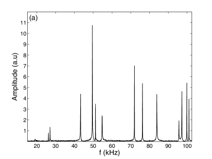
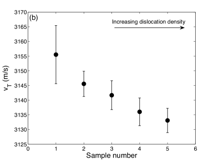
Figure 1: (a) Typical frequency spectrum, showing the first 14 resonances for sample N^∘ 3 of Table I. The first resonant mode is at $\approx 18$ kHz, the last one at $\approx 101$ kHz. (b) Shear wave velocity for the five samples under study. The arrow indicates the direction in which dislocation density is expected to increase.

Resonant Ultrasound Spectroscopy allows precise measurements of the elastic constants of a sample independent of its symmetries [Migliori et al., 1993; Leisure & Willis 1997]. An homogeneous and isotropic material is characterized by two independent elastic constants, $\lambda$ and $\mu$, or equivalently $C_{11}=\rho v_{L}^{2}$ and $C_{44}=\rho v_{T}^{2}$. RUS is known to give more precise measurements of $C_{44}$, and therefore a comparison with the theoretical prediction for $v_{T}$ is possible.

We have taken five aluminum samples cut from the same bar. One, as bought, one cold-rolled at 33%, one cold rolled at 43%, one annealed at 400^∘C, for 5 hours, and another for 10 hours. Longer annealing means lower dislocation density, and stronger cold-rolling means higher dislocation density. The five samples were shaped as parallelepipeds, with dimensions as in Table I. Samples are labeled $1,2,3,4$ and $5$ for increasing expected density dislocation. A RUS apparatus was built in-house [Carú, 2007; Jara, 2007], and used to measure the two elastic constants of the five samples. The sample-apparatus contact force is small, of the order of $0.1$ N. A typical spectrum is shown in Figure 1a. Each resonant frequency was measured for several ultrasonic driving amplitudes (typically five) in order to verify that the resonances are well in the linear acoustic regime. Additionally, each sample was placed five times in the apparatus in order to reduce errors due to slight dependence of the resonant frequencies on the contact load and positioning with respect to the ultrasonic receiver. The measured elastic constants $C_{11}$ and $C_{44}$ as well as the shear and longitudinal wave velocities are also given in Table I. No clear tendency in $v_{L}$ is observed. Within experimental errors, it is almost constant. However, $v_{T}$ shows a clear decreasing tendency. It is plotted in Figure 1b versus sample number. The difference between the errors of both wave velocities is consistent with the fact that RUS is much more precise for $C_{44}$, basically because resonant frequencies depend strongly on $C_{44}$ and weakly on $C_{11}$.

IV Discussion and conclusions

For simplicity we shall assume, a common assumption, $\lambda=\mu$, so that $\gamma^{2}=3$. Independent measurements for the original sample give $\gamma^{2}=3.3$, and this ratio does not change significantly from sample to sample.

Using (3) we have

$$\frac{\mu b^{2}}{\Gamma}=\frac{4\pi\gamma^{2}}{\gamma^{2}-1}\ln^{-1}\left(\frac{\delta}{\delta_{0}}\right)$$

so there is only a dependence on the ratio of cut-offs. Taking $\delta=10^{6}\delta_{0}$ we get the following expression for the fractional change in shear wave velocity:

$$\frac{v_{T}-c_{T}}{c_{T}}=-\frac{16}{5\pi^{3}}\frac{3}{2}\frac{nL^{3}}{6\ln 10}.$$ (15)

The data of Figure 1b are consistent with

$$nL^{3}\sim 0.3$$ (16)

and with a (linear) trend in agreement with theory, namely that the higher the dislocation density, the lower the effective speed of shear waves.

Taking $L\sim 100$ nm as a typical dislocation length would give a variation in dislocation density among the various samples of order $nL\sim 10^{9}$ mm^-2, a conclusion that it should be possible to test by direct measurement with High Resolution Transmission Electron Microscopy (HRTEM). Work along this direction is in progress.

References

Arakawa, K., Hatakana, M., Kuramoto, E., Ono, K. & H. Mori, H. [2006], “Changes in the Burgers Vector of Perfect Dislocation Loops without Contact with the External Dislocations”, Phys. Rev. Lett. 96, 125506.

Carú, A. [2007], “Caracterización Acústica de Materiales”, Acoustics Engineering thesis, Universidad Austral de Chile.

Granato, A. V., & Lücke, K. [1956a], “Theory of Mechanical damping due to dislocations”, J. Appl. Phys. 27, 583-593.

Granato, A. V., & Lücke, K. [1956b], “Application of dislocation theory to internal friction phenomena at high frequencies”, J. Appl. Phys. 27, 789-805.

Granato, A. V., & Lücke, K. [1966], in Physical Acoustics, Vol 4A, edited by W. P. Mason (Academic).

Jara, A. [2007], “Caracterización acústica de diferentes muestras de aluminio”, (unpublished).

Koehler, J. S. [1952], in Imperfections in nearly Perfect Crystals, edited by W. Schockley et al. (Wiley).

Ledbetter, H. M. & Fortunko, C. [1995], “Elastic constants and internal friction of polycrystalline copper”, J. Mater. Res. 10, 1352-1353.

Leisure, R. G. & Willis, F. A. [1997], “Resonant ultrasound spectroscopy”, J. Phys. Condens. Matter 9, 6001-6029.

Lund, F. [1988], “Response of a stringlike dislocation loop to an external stress”, J. Mat. Res. 3, 280-297.

Maurel, A., Mercier, J.-F., & Lund, F. [2004a], “Scattering of an elastic wave by a single dislocation”, J. Acoust. Soc. Am. 115, 2773-2780.

Maurel, A., Mercier, J.-F. & Lund, F. [2004b], “Elastic wave propagation through a random array of dislocations”, Phys. Rev. B 70, 024303.

Maurel, A., Pagneux, V., Barra, F. & Lund, F. [2005a] “Interaction between an elastic wave and a single pinned dislocation” Phys. Rev. B 72, 174110.

Maurel, A., Pagneux, V., Barra, F. & Lund, F. [2005b] “Wave propagation through a random array of pinned dislocations: Velocity change and attenuation in a generalized Granato and Lücke theory”, Phys. Rev. B 72, 174111.

Maurel, A., Pagneux, V., Boyer, D., & Lund, F. [2006] “Propagation of elastic waves through polycrystals: the effects of scattering from dislocation arrays”, Proc. R. Soc. Lond. A, 462, 2607-2623.

Maurel, A., Pagneux, V., Barra, D. & Lund, F. [2007a], “Interaction of a Surface Wave with a Dislocation”, Phys. Rev. B 75, 224112.

Maurel, A., Pagneux, V., Barra, D. & Lund, F. [2007b] “Multiple scattering from assemblies of dislocation walls in three dimensions. Application to propagation in polycrystals”, J. Acoust. Soc. Am., 121, 3418-3431.

Migliori, A., Sarrao, J. L., Visscher, William M., Bell, T. M., Lei, Ming, Fisk, Z. & Leisure, R. G. [1993] “Resonant ultrasound spectroscopic techniques for measurement of the elastic moduli of solids”, Physica B 183, 1-24.

Ogi, H., Ledbetter, H.M., Kim, S. & Hirao, M. [1999], “Contactless mode-selective resonance ultrasound spectroscopy: Electromagnetic acoustic resonance”, J. Acoust. Soc. Am. 106, 660-665.

Ogi, H., Nakamura, N., Hirao, M. & Ledbetter, H. [2004], “Determination of elastic, anelastic, and piezoelectric coefficients of piezoelectric materials from a single specimen by acoustic resonance spectroscopy”, Ultrasonics 42, 183-187.

Ohtani, T., Ogi, H. & Hirao, M. [2005], “Acoustic damping characterization and microstructure evolution in nickel-based superalloy during creep”, Int. J. Sol. and Struct. 42, 2911-2928.

Peach, M. O., & Koehler, J. S. [1950], “The Forces Exerted on Dislocations and the Stress Fields Produced by them”, Phys. Rev., 80, 436-439.

Robertson, I. A., Ferreira, P. J., Dehm, G., Hull, R. & Stach, E. A. [2008], “Visualizing the Behavior of Dislocations—Seeing is Believing”, MRS Bulletin 33, 122-131.

Stix, T. H. [1992], Waves in Plasmas, Springer.

Williams, D. B., & Carter, C. B. [2004], Transmission Electron Microscopy: A Textbook for Materials Science (Springer, 2004).