Global solutions in gravity.
Euclidean signature.

Abstract

We consider a wide class of two-dimensional metrics having one Killing vector. The method is proposed for the construction of maximally extended surfaces with the given Riemannian metric which is the analog of the conformal block method for two-dimensional Lorentzian signature metrics. The Schwarzschild solution is considered as an example.

1 Introduction

For physical interpretation of solutions in different gravity models, one has not only to find the metric as a solution of the equations of motion but also to analyze the behavior of extremals (geodesics) corresponding, in particular, to trajectories of point particles. Therefore the construction of global solutions is of uttermost significance. By global solution we mean a pair $({\mathbb{M}},g)$ where ${\mathbb{M}}$ is a manifold and $g=\{g_{\alpha\beta}\}$ is a metric given on ${\mathbb{M}}$. The metric is to be found as a solution to some system of the Euler–Lagrange equations and a manifold is supposed to be maximally extended. The last requirement means that any extremal can be prolonged either to infinite value of the canonical parameter in both directions or it ends up at a singular point at a finite value of the canonical parameter where at least one of the geometric invariants is infinite or not defined. The well known example is the Kruskal–Szekerez extension of the Schwarzschild solution [1, 2].

In general, this problem is very complicated because it requires an exact solution of the equations of motion as well as the analysis of extremals. The case of spherically symmetric solutions in general relativity was analyzed by Carter in [3]. The method of conformal blocks for constructions of global solutions for a wide class of two-dimensional metrics having one Killing vector was proposed in [4]. This method was developed as a result of construction and classification of all global solutions [5, 6, 7] in two-dimensional gravity with torsion [8, 9, 10]. The method of conformal blocks was also used for construction of global solutions in many two-dimensional dilaton gravity models [11, 12] and for complete classification of global vacuum solutions in general relativity with a cosmological constant assuming that the four-dimensional space-time is a warped product of two surfaces with a block diagonal metric [13]. In the last case, all solutions were known locally. The analysis of global properties gave physical interpretation of many solutions which were earlier known only locally. Besides the black hole solutions, the vacuum Einstein equations have solutions describing cosmic strings, domain walls of curvature singularities, cosmic strings surrounded by domain walls, and other physically interesting solutions.

The method of conformal blocks is applicable for metrics of Lorentzian signature. At the same time, the Euclidean formulation of the theory plays important role in quantum field theory and statistical mechanics and allows in some cases to avoid difficulties related to the indefinite signature of the metric. In the present paper, the method of conformal blocks is generalized to a wide class of two-dimensional metrics of Euclidean signature having one Killing vector. We prove that there is the global solution for each conformal block with positive or negative definite metric. This method was applied earlier to two-dimensional gravity with torsion [14] and in the analysis of hyperbolically symmetric solutions in general relativity [13].

2 Local form of the metric

We start with the Lorentz case to explain the choice of the Riemannian metric for the present paper. At first glance, the choice of Lorentzian metric may seem artificial, but many exact solutions of general relativity depending essentially on two coordinates can be written in this way. Besides, a general solution of the equations of motion of two-dimensional gravity has exactly this form in the conformal gauge [15].

We consider a plane ${\mathbb{R}}^{2}$ with Cartesian coordinates $x^{\alpha}=\{\tau,\sigma\}$, $\alpha=1,2$. Two-dimensional metrics of constant curvature as well as many solutions of general relativity and other gravity models can be written in the form [4]

$$ds^{2}=|N(q)|(d\tau^{2}-d\sigma^{2}).$$ (1)

where the conformal factor $N(q)\in{\cal C}^{l}$, $l\geq 2$, is $l$ times continuously differentiable function of one variable $q\in{\mathbb{R}}$ except finite number of singularities. Let variable $q$ depend only on one coordinate, the dependence being given by the ordinary differential equation

$$\left|\frac{dq}{d\zeta}\right|=\pm N(q),$$ (2)

with the following sign rule

$$\begin{array}[]{ccl}N>0:&~{}~{}\zeta=\sigma,&~{}~{}\text{$+$ sign (static solution)},\\ N<0:&~{}~{}\zeta=\tau,&~{}~{}\text{$-$ sign (homogeneous solution)}.\end{array}$$ (3)

Equations (1) and (2) define four different metrics due to the modulus and $\pm$ signs in Eq.(2). There are two surfaces with static metrics and two surfaces with homogeneous metrics which differ by the sign of the derivative $dq/d\zeta$. Let us denote these domains by the Roman numbers,

$$\begin{array}[]{rcl}\text{I}:{}{}&N>0,{}{}&dq/d\sigma>0,\\ \text{II}:{}{}&N<0,{}{}&dq/d\tau<0,\\ \text{III}:{}{}&N>0,{}{}&dq/d\sigma<0,\\ \text{IV}:{}{}&N<0,{}{}&dq/d\tau>0.\end{array}$$ (4)

To clarify the form of the metric (1), we note that in domain I there are Schwarzschild like coordinates $\tau,q$ in which the metric becomes

$$ds^{2}=N(q)d\tau^{2}-\frac{dq^{2}}{N(q)}.$$

So the variable $q$ can be interpreted there as the radius and the conformal factor as the $g_{00}$ component of the metric.

To transform Lorentzian metric (1) to the Euclidean signature metric, we perform the rotation in the complex plane of the coordinate on which the conformal factor does not depend. The corresponding Riemannian metric is the solution of the same system of the Euler–Lagrange equations as the original Lorentzian metric (1) because the conformal factor does not depend on this coordinate. This transformation is given by the coordinate changes $\tau=i\rho$ and $\sigma=i\rho$ in domains I,III and II,IV, respectively. As a result, we obtain the metric

$$ds^{2}=-N(q)(d\sigma^{2}+d\rho^{2}),$$ (5)

where we changed notations $\tau\rightarrow\sigma$ in domains II and IV. The sign of the conformal factor $N(q)$ is not fixed, and we consider both positive and negative definite metrics. After the transformation the variable $q$ depends only on $\sigma$, this dependence being given by the ordinary differential equation

$$\left|\frac{dq}{d\sigma}\right|=\left|N(q)\right|.$$ (6)

The modulus signs are opened in the following way

$${\rm I:} N>0,~{}~{}~{}~{}dq/d\sigma >0, {\sf\,sign\,}g_{\alpha\beta} =(--),$$ (7)

$${\rm II:} N<0,~{}~{}~{}~{}dq/d\sigma <0, {\sf\,sign\,}g_{\alpha\beta} =(++),$$

$${\rm III:} N>0,~{}~{}~{}~{}dq/d\sigma <0, {\sf\,sign\,}g_{\alpha\beta} =(--),$$

$${\rm IV:} N<0,~{}~{}~{}~{}dq/d\sigma >0, {\sf\,sign\,}g_{\alpha\beta} =(++),$$

where the signature of the metric (5) is shown in the last column. Metrics in domains I and III as well as in domains II and IV are essentially the same because they are related by the transformation $\sigma\rightarrow-\sigma$.

Riemannian metric defined by Eqs.(5) and (6) is the subject of the present paper. We admit the conformal factor to have zeroes and singularities at a finite number of points $q_{i}$, $i=1,\dots,k$. Infinite points $q_{1}=-\infty$ and $q_{k}=\infty$ are included in this sequence. In this way the real line $q$ is divided on intervals by points $q_{i}$ in which the conformal factor is either strictly positive or negative. We consider power behavior of the conformal factor near the boundary points $q_{i}$:

$$|q_{i}|<\infty: N(q)\sim|q-q_{i}|^{m},$$ (8)

$$|q_{i}|=\infty: N(q)\sim|q|^{m}.$$ (9)

For finite $q_{i}$, the exponent differs from zero, $m\neq 0$, because the conformal factor either equals zero or singular by assumption. In a general case, the exponent $m$ can be an arbitrary real number. Horizons of the space-time correspond to zeroes of the conformal factor at finite points $|q_{i}|<\infty$ in the Lorentzian case [5].

Metric (5) has at least one Killing vector $K=\partial_{\rho}$, its length being $-N(q)$.

Christoffel’s symbols are defined by the metric,

$$\Gamma_{\alpha\beta}{}^{\gamma}=g^{\gamma\delta}(\partial_{\alpha}g_{\beta\delta}+\partial_{\beta}g_{\alpha\delta}-\partial_{\delta}g_{\alpha\beta}),$$

and have the following nontrivial components

$${\rm I,II}: ~{}~{}~{}~{}~{}~{}\Gamma_{\sigma\sigma}{}^{\sigma}=\Gamma_{\sigma\rho}{}^{\rho}=\Gamma_{\rho\sigma}{}^{\rho}=-\Gamma_{\rho\rho}{}^{\sigma}=\frac{1}{2}N^{\prime},$$ (10)

$${\rm III,IV}: ~{}~{}~{}~{}~{}~{}\Gamma_{\sigma\sigma}{}^{\sigma}=\Gamma_{\sigma\rho}{}^{\rho}=\Gamma_{\rho\sigma}{}^{\rho}=-\Gamma_{\rho\rho}{}^{\sigma}=-\frac{1}{2}N^{\prime},$$ (11)

where prime denotes the derivative with respect to the argument, $N^{\prime}=dN/dq$, and there is no summation over indices $\rho$ and $\sigma$. The curvature tensor in our notations is

$$R_{\alpha\beta\gamma}{}^{\delta}=\partial_{\alpha}\Gamma_{\beta\gamma}{}^{\delta}-\Gamma_{\alpha\gamma}{}^{\epsilon}\Gamma_{\beta\epsilon}{}^{\delta}-(\alpha\leftrightarrow\beta).$$

It is the same in all domains and has only one independent component

$$R_{\sigma\rho\sigma}{}^{\rho}=\frac{1}{2}NN^{\prime\prime}$$ (12)

Nonzero components of the Ricci tensor and the scalar curvature are

$$R_{\sigma\sigma} =R_{\rho\rho}=\frac{1}{2}NN^{\prime\prime},$$ (13)

$$R =-N^{\prime\prime}.$$ (14)

As the consequence, the conformal factor $N$ is the second power polynomial for constant curvature surfaces $R={\sf\,const}$.

According to Eq.(14), the scalar curvature is singular at $q_{i}$ for the following exponents in the power behavior in Eq.(8):

$$|q_{i}|<\infty: m<0,~{}~{}0<m<1,~{}~{}1<m<2,$$ (15)

$$|q_{i}|=\infty: m>2.$$ (16)

At infinite boundary points $q_{i}=\pm\infty$ the scalar curvature goes to nonzero constant for $m=2$ and to zero for $m<0$. Note that the nonzero value of the scalar curvature at finite points $|q_{i}|<\infty$ can occur also for $m=1$ due to the next power corrections in expansion (8).

The range of definition for metric (5) on the $\sigma,\rho$ plane depends on the conformal factor. Coordinate $\rho\in{\mathbb{R}}$ runs through all real line because nothing depends on it, but the range of definition of coordinate $\sigma$ is defined by Eq.(6). We have finite, semifinite or infinite interval for coordinate $\sigma$ in the each interval $q\in(q_{i},q_{i+1})$ depending on whether the integral

$$\sigma\sim\int^{q_{i},q_{i+1}}\frac{dq}{N(q)}$$ (17)

converge or diverge at the boundary points. Depending on the exponent $m$ we have

$$\begin{array}[]{rl}|q_{i}|<\infty:{}{}{}{}&\left\{\begin{array}[]{rll}m<1,{}{}&\text{converge,}\\ m\geq 1,{}{}&\text{diverge,}\end{array}\right.\\ |q_{i}|=\infty:{}{}{}{}&\left\{\begin{array}[]{rll}m\leq 1,{}{}&\text{diverge,}\\ m>1,{}{}&\text{converge,}\end{array}\right.\end{array}$$ (18)

Coordinate $\sigma$ runs through all real line, $\sigma\in(-\infty,\infty)$ if the integral diverge at both ends of the interval $(q_{i},q_{i+1})$, and the metric is defined on the whole plane $\sigma,\rho\in{\mathbb{R}}^{2}$. If at one boundary point $q_{i+1}$ or $q_{i}$ the integral converge, then the metric is defined on the half plane $\sigma\in(-\infty,\sigma_{i+1})$ or $\sigma\in(\sigma_{i},\infty)$, respectively. The choice of boundary points $\sigma_{i+1}$ and $\sigma_{i}$ is arbitrary, and without loss of generality, we can put $\sigma_{i,i+1}=0$. If the integral converges at both boundary points, then the solution is defined on the strip $\sigma\in(\sigma_{i},\sigma_{i+1})$, and only one of the ends of the interval can be set to zero.

To construct the maximally extended surface in the Lorentzian case, we attribute the conformal block of definite shape to each interval $(q_{i},q_{i+1})$ and then glue them together. For the Euclidean signature metric, there is no need for this procedure because “lightlike” extremals with asymptotics $\rho=\pm\sigma+{\sf\,const}$ are shown to be absent.

The value of variable $q$ and hence the scalar curvature are constant along Killing trajectories $\sigma={\sf\,const}$. Variable $q$ is monotonically increasing on $\sigma$ in domains I,IV and monotonically decreasing in domains II,III according to the definition of the domains (7).

3 Extremals

To describe maximally extended surface for metric (5) we must analyze the behavior of extremals $x^{\alpha}(t)=\{\sigma(t),\rho(t)\}$, $t\in{\mathbb{R}}$ given by the system of ordinary differential equations

$$\ddot{x}^{\alpha}=-\Gamma_{\beta\gamma}{}^{\alpha}\dot{x}^{\beta}\dot{x}^{\gamma},$$

where dot denotes the derivative with respect to the canonical parameter $t$ which is defined up to a linear transformation. For definiteness, consider domain I. Expressions for Christoffel’s symbols (10) yield the system of equations for extremals

$$\ddot{\sigma} =\frac{1}{2}N^{\prime}(\dot{\rho}^{2}-\dot{\sigma}^{2}),$$ (19)

$$\ddot{\rho} =-N^{\prime}\dot{\sigma}\dot{\rho}.$$ (20)

It has two first integrals

$$-N(\dot{\sigma}^{2}+\dot{\rho}^{2}) =C_{0}={\sf\,const},$$ (21)

$$-N\dot{\rho} =C_{1}={\sf\,const}.$$ (22)

The existence of the integral (21) allows one to choose the length of the extremal as a canonical parameter. The second integral (22) is connected to the existence of the Killing vector. Now we formulate the theorem determining extremals.

Theorem 3.1.

Any extremal in domain I belongs to one of the four classes.
1. Straight extremals of the form (the analog of lightlike extremals)

$$\rho=\pm\sigma+{\sf\,const},$$ (23)

exist only for the Euclidean metric $N={\sf\,const}$ and the canonical parameter can be chosen as $\sigma=t$.
2. General type extremals which form is defined by equation

$$\frac{d\rho}{d\sigma}=\pm\frac{1}{\sqrt{-1-C_{2}N}},$$ (24)

where $C_{2}$ is a negative constant. Canonical parameter is defined by any of the equations

$$\dot{\sigma} =\pm\frac{\sqrt{-1-C_{2}N}}{N},$$ (25)

$$\dot{\rho} =\frac{1}{N}.$$ (26)

The signs plus or minus in Eqs.(24) and (25) must be chosen simultaneously.
3. Straight extremals parallel to axis $\sigma$ and going through each point $\rho={\sf\,const}$. Canonical parameter is defined by equation

$$\dot{\sigma}=\frac{1}{\sqrt{N}}.$$ (27)

4. Straight degenerate extremals parallel to axis $\rho$ and going through the points $\sigma_{0}={\sf\,const}$ in which

$$N^{\prime}(\sigma_{0})=0.$$ (28)

Canonical parameter can be chosen as

$$t=\rho.$$ (29)

The proof of this theorem repeats almost word by word the proof of the corresponding theorem in the Lorentzian case [4] and is not given here. Let us remind that constant $C_{2}$ is defined by the integrals (21) and (22)

$$C_{2}=\frac{C_{0}}{C_{1}^{2}}.$$ (30)

Equation (24) shows that constant $C_{2}$ parameterizes the angle at which an extremal of general type goes through a given point.

Behavior of extremals for metrics with Euclidean signature is essentially different from that for Lorentzian metrics. First, the analog of lightlike extremals is absent for Riemannian metrics. This is important because lightlike extremals are incomplete on horizons and must be continued. This problem is absent in the Riemannian case. Second, Eqs.(24) and (25) differ from the corresponding equations in the Lorentzian case by the sign before the unity inside the square root. At first glance insignificant, this difference leads to the absence of “lightlike” asymptotics for extremals of general type as $q\rightarrow q_{i}$ near zeroes of conformal factor $N(q_{i})=0$ which define horizons.

Qualitative behavior of extremals of general type is easily analyzed. We consider domain I for definiteness. The conformal factor is positive in domain I, and extremals of a general type exist only for negative values of the constant $C_{2}$ because otherwise the right hand side of Eq.(26) becomes imaginary. The inequality

$$N(q)\geq-1/C_{2}.$$

must hold. For sufficiently large values of the modulus of $C_{2}$, this inequality determines the range of $q\in(q^{\prime},q^{\prime\prime})$ where the boundary points $q^{\prime}$ and $q^{\prime\prime}$ are given by equations $N(q)=-1/C_{2}$. This range definits points $\sigma^{\prime}$ and $\sigma^{\prime\prime}$ which correspond to $q^{\prime}$ and $q^{\prime\prime}$. The extremal of general type can not go out of the strip $\sigma\in(\sigma^{\prime},\sigma^{\prime\prime})$, $\rho\in(-\infty,\infty)$. Simple analysis of Eq.(26) shows that extremals of general type oscillate between the values $\sigma^{\prime}$ and $\sigma^{\prime\prime}$ as shown in Fig.1$a_{3}$,$b_{3}$. Oscillating extremals of general type are always complete because the right hand side of Eq.(26) is bounded from the top by $1/N(q^{\prime})$ or $1/N(q^{\prime\prime})$ and bottom by $1/{\sf\,max\,}N(q)$.

If the conformal factor is equal to infinity in point $q_{i+1}$ as shown in Fig.1$b$, then an extremal of general type can start and end at the singular boundary. This boundary corresponds to finite value $\sigma_{i+1}$ for $|q_{i+1}|<\infty$, $m<1$ and $|q_{i+1}|=\infty$, $m>1$. All these extremals approach the singular boundary at right angle because the right hand side of Eq.(24) goes to zero. Completeness of extremals of general type going to the singular boundary is defined by the integral

$$\lim_{q\to q_{i+1}}t\to\int^{q_{i+1}}\frac{dq}{\sqrt{N}},$$ (31)

as the consequence of Eqs.(25) and (6). So completeness of extremals of general type which approach the singular boundary is the same as completeness of straight extremals parallel to axis $\sigma$ (27). They are complete only for $|q_{i+1}|=\infty$ and $1<m\leq 2$.

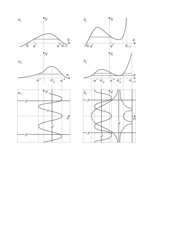
Figure 1: Top row ($a_{1}$, $b_{1}$): typical behavior of the conformal factor $N(q)$ between two zeroes and a zero and singularity. Middle row ($a_{2}$, $b_{2}$): dependence of the conformal factor $N(\sigma)$ on coordinate $\sigma$. Point $\sigma_{i+1}$ can be either at finite or infinite distance from the origin. Bottom row ($a_{3}$, $b_{3}$): extremals of general type ($o$) for different values of $C_{2}$ oscillate between $\sigma^{\prime}$ and $\sigma^{\prime\prime}$ near local maximum. There is one degenerate extremal ($d$) which goes through every local extremum. There are extremals ($s$) that asymptotically approach the degenerate extremal at local minimum $\sigma^{\prime}_{0}$ and can end at the singular boundary $\sigma_{i+1}$. Extremals of general type ($r$) of finite length start and end at the singular boundary. All extremals can be arbitrary moved along axis $\rho$. Straight extremals ($p$) parallel to axis $\sigma$ are going through every point $\rho$.

Typical behavior of the conformal factor between two zeroes and with two local extrema between zero and singularity is shown in the top row of Fig.1, ($a_{1}$, $b_{1}$). In case 1$b$ we assume $|q_{i+1}|<\infty$ and $m<1$ or $1<m<2$ corresponding to the curvature singularity. In the middle row ($a_{2}$, $b_{2}$), we shaw the dependence of the conformal factors on coordinate $\sigma$. The value of coordinate $\sigma_{i+1}$ is finite for $m<1$ and infinite for $1<m<2$ in Fig.1,$b_{2}$. Qualitative behavior of extremals on the $\sigma,\rho$ plane is shown in the bottom row ($a_{3}$, $b_{3}$). Extremals of general type $(o)$ oscillate near local maximum $N(\sigma_{0})$ between $\sigma^{\prime}$ and $\sigma^{\prime\prime}$ which are determined by the value of constant $C_{2}$. These extremals $(r)$ can also start and end at the singular boundary $\sigma_{i+1}$ having a finite length. Degenerate extremals $(d)$ go through every extremum of the conformal factor. There are also extremals of general type $(s)$ which asymptotically approach the degenerate extremal going through local minimum $\sigma^{\prime}_{0}$ when $\rho\to\pm\infty$. Part of these extremals end at the singular boundary $\sigma_{i+1}$ at a finite value of the canonical parameter. All extremals can be shifted arbitrary along axis $\rho$. Straight extremals $(p)$ parallel to axis $\sigma$ go through every point $\rho$.

If both boundary points $q_{i}$ and $q_{i+1}$ of the interval are zeroes, then the conformal factor $N$ has at least one maximum as the consequence of continuity through which goes the degenerate extremal ($d$). Degenerate extremals are always complete, i.e. have infinite length, because the canonical parameter coincides with coordinate $\rho$ (29).

The above analysis shows that incompleteness of extremals in strips $\sigma\in(\sigma_{i},\sigma_{i+1})$ and $\rho\in(-\infty,\infty)$ is defined entirely by completeness of straight extremals parallel to axis $\sigma$ when they approach boundary points $\sigma_{i},\sigma_{i+1}$. In its turn, this is defined by the convergence of the integral (31). These extremals are incomplete at finite points $|q_{i}|<\infty$ for $m<2$. At infinite points $|q_{i}|=\infty$ they are incomplete for $m>2$ and complete in all other cases. Extension of the surface is necessary only for the conformal factor which has simple zero $m=1$ at a finite point $q_{i}$ because we must extend the surface only for nonsingular curvature. Note that a simple zero in the Lorentzian case corresponds to a horizon, and this is the unique case when four conformal blocks meet at a saddle point. The Carter–Penrose diagram for the Schwarzschild solution has exactly this form.

4 Global solutions

To construct maximally extended surfaces with metric (5), we perform the following procedure which is useful also for visualization of the surfaces. We identify points $\rho$ and $\rho+L$ where $L$ is an arbitrary positive constant which is always possible because nothing depends on coordinate $\rho$. After this identification the plane $\sigma,\rho$ becomes a cylinder. The circumference of the directing circle is equal to

$$P=LN(q)\rightarrow\begin{cases}0,&N(q_{i})=0,\\ \infty&N(q_{i})=\infty.\end{cases}$$ (32)

The plane $\sigma,\rho$ is the universal covering space for this cylinder.

We summarize properties of the boundary points $q_{i}$ in Table 1.

$|q_{i}|<\infty$
	$m<0$	$0<m<1$	$m=1$	$1<m<2$	$m=2$	$m>2$
$R$	$\infty$	$\infty$	${\sf\,const}$	$\infty$	${\sf\,const}$	$0$
$\sigma_{i}$	${\sf\,const}$	${\sf\,const}$	$\infty$	$\infty$	$\infty$	$\infty$
$P$	$\infty$	$0$	$0$	$0$	$0$	$0$
Completeness	$-$	$-$	$-$	$-$	$+$	$+$
$|q_{i}|=\infty$
	$m<0$	$m=0$	$0<m\leq 1$	$1<m<2$	$m=2$	$m>2$
$R$	$0$	$0$	$0$	$0$	${\sf\,const}$	$\infty$
$\sigma_{i}$	$\infty$	$\infty$	$\infty$	${\sf\,const}$	${\sf\,const}$	${\sf\,const}$
$P$	$0$	${\sf\,const}$	$\infty$	$\infty$	$\infty$	$\infty$
completeness	$+$	$+$	$+$	$+$	$+$	$-$

Table 1: Properties of boundary points depending on the exponent $m$. The symbol ${\sf\,const}$ in the rows for the scalar curvature denotes a nonzero constant.

Depending on the value of the exponent $m$, we show there the values of scalar curvature $R$ on the corresponding surface, finiteness of coordinate $\sigma_{i}$ at the point $q_{i}$, circumference of directing circles for cylinders $P$ and completeness of extremals which are parallel to axis$\sigma$.

Forms of the surfaces near boundary points $q_{i+1}$ after the identification $\rho\sim\rho+L$ are shown in Fig.2. Surfaces near points $q_{i}$ have similar form but are turned in the opposite direction. The surface corresponding to the whole interval $(q_{i},q_{i+1})$ is obtained by gluing two such surfaces for boundary points $q_{i}$ and $q_{i+1}$ together.

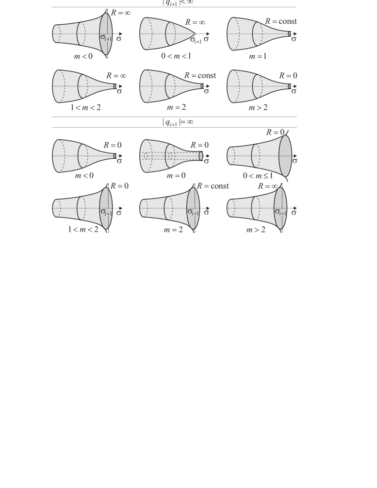
Figure 2: Forms of the surfaces near boundary points $q_{i+1}$ after the identification $\rho\sim\rho+L$. By assumption, the coordinate $\sigma$ grows from left to right and $\sigma_{i+1}>\sigma_{i}$. Surfaces near points $q_{i}$ have a similar form but are turned in the opposite direction. The surface for the whole interval $q_{i},q_{i+1}$ is obtained by gluing two such surfaces for boundary points $q_{i}$ $q_{i+1}$ together.

So extremals must be continued only near the boundary point $|q_{i}|<\infty$ for $m=1$. We call this point horizon because it corresponds to a horizon in the Lorentzian case. The continuation at a horizon is performed as follows. First of all note that a horizon in the Euclidean case is itself a point because the length of the directing circle goes to zero. Next, this “infinite” point in the $\rho,\sigma$ plane lays, in fact, at a finite distance because all extremals reach this point at a finite value of the canonical parameter. Up to higher order terms, the conformal factor in the neighborhood of the point $q_{i}$ has the form

$$N(q)=N^{\prime}_{i}(q-q_{i}),$$ (33)

where $N^{\prime}_{i}=N^{\prime}(q_{i})={\sf\,const}\neq 0$. In domain I for $N^{\prime}_{i}>0$ and $q>q_{i}$, Eq.(6) is easily integrated

$$q-q_{i}=e^{N^{\prime}_{i}\sigma},$$

where we dropped an insignificant constant of integration related to a shift of $\sigma$. Thus the boundary point $|q_{i}|<\infty$ is reached for $\sigma\rightarrow-\infty$. Metric (5) in coordinates $q,\rho$ which play the role of Schwarzschild coordinates takes the form

$$-ds^{2}=\frac{dq^{2}}{N^{\prime}_{i}(q-q_{i})}+N^{\prime}_{i}(q-q_{i})d\rho^{2}.$$ (34)

In polar coordinates $r,\varphi$, defined by the transformation

$$q-q_{i}=\frac{N^{\prime}_{i}}{4}r^{2},~{}~{}~{}~{}~{}~{}\rho=\frac{2}{N^{\prime}_{i}}\varphi,$$ (35)

the metric becomes Euclidean

$$-ds^{2}=dr^{2}+r^{2}d\varphi^{2}.$$

Here the polar angle varies within the interval $\varphi\in(0,LN^{\prime}_{i}/2)$ and the radius $r$ is defined in the neighborhood of the boundary point $q_{i}$ by Eq.(35). This coordinate transformation maps the “infinite” line $\sigma_{i}=-\infty$, $\rho\in{\mathbb{R}}$ into the origin of Euclidean plane. Conical singularity can appear at the origin because the polar angle varies within the interval which in general differs from $(0,2\pi)$. The corresponding deficit angle is

$$2\pi\theta=\frac{LN^{\prime}_{i}}{2}-2\pi.$$ (36)

Thus we get the Euclidean metric on a plane ${\mathbb{R}}^{2}$ with a conical singularity at the origin. The deficit angle is zero for $L=4\pi/N^{\prime}_{i}$, conical singularity is absent, and we are left with the flat Euclidean metric which is evidently smooth at the origin. In general, conformal factor (33) has corrections of higher order near the boundary point $q_{i}$ and transformation to polar coordinates yields the metric of the same differentiability as the conformal factor.

In general continuation of the solution through the point $|q_{i}|<\infty$ for $m=1$ has no meaning because this point correspond to a conical singularity. We assume that this point as well as any other singular point does not belong to a manifold. Therefore the plane $\sigma,\rho$ or its part is the universal covering space for the surface with metric (5). Continuation is necessary only in the absence of conical singularity $L=4\pi/N^{\prime}_{i}$. In this case, straight extremals parallel to axis $\sigma$ and going through points $\rho$ and $\rho+L/2$ become two halves of the same extremal shown in Fig.3. The fundamental group is trivial in the absence of a conical singularity, and therefore the corresponding surface is itself a universal covering space.

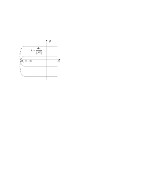
Figure 3: Continuation of straight extremals going through points $\rho$ and $\rho+L/2$ in the absence of conical singularity $L=4\pi/|N^{\prime}_{i}|$. The identification is performed in the point $\sigma_{i}=-\infty$.

If the conformal factor has asymptotics $N\sim(q-q_{i})$ and $N\sim(q_{i+1}-q)$ on both sides of the interval $(q_{i},q_{i+1})$, then the surface must be continued in both points $\sigma=\pm\infty$. In general, after the identification $\rho\sim\rho+L$ the surface has conical singularities in both points. For $LN^{\prime}_{i}=4\pi$ and $LN^{\prime}_{i+1}=4\pi$ conical singularities are absent. There are three types of global surfaces shown in Fig.4 according to the number of conical singularities. These surfaces have topology of a cylinder, plane or sphere, respectively.

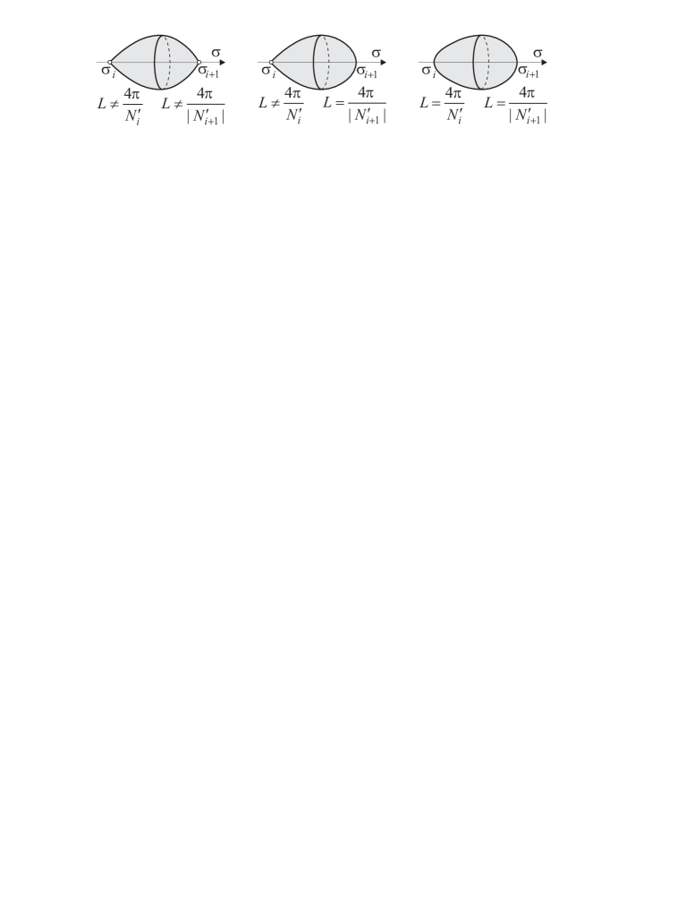
Figure 4: Three types of possible maximally extended surfaces, corresponding to the interval $(q_{i},q_{i+1})$ when the conformal factor has asymptotics $N\sim(q-q_{i,i+1})$ in boundary points. In general, the surface has two conical singularities after the identification $\rho\sim\rho+L$. For $L|N^{\prime}_{i,i+1}|=4\pi$ conical singularities are absent.

The rules for construction of maximally extended surfaces with metric (5) are as follows.

1. The maximally extended surface corresponds to each interval $(q_{i},q_{i+1})$ after the identification $\rho\sim\rho+L$ and is obtained by gluing of two surfaces shown in Fig.2 corresponding to the boundary points $q_{i}$ and $q_{i+1}$.

2. In all cases except the absence of the conical singularity, $|q_{i}|<\infty$, $LN^{\prime}_{i}\neq 4\pi$ or $|q_{i+1}|<\infty$, $L|N^{\prime}_{i+1}|\neq 4\pi$ the strip $\sigma\in(\sigma_{i},\sigma_{i+1})$, $\rho\in{\mathbb{R}}$ with metric (5) is the universal covering space for the corresponding maximally extended surface.

3. In the absence of one of conical singularities, $|q_{i}|<\infty$, $LN^{\prime}_{i}=4\pi$ or $|q_{i+1}|<\infty$, $L|N^{\prime}_{i+1}|=4\pi$, the surface obtained from the plane $\sigma,\rho$ by identification $\rho\sim\rho+L$ is itself the maximally extended surface with trivial fundamental group.

Note that we do not glue together coordinate charts. It means that the corresponding surfaces are smooth ${\cal C}^{\infty}$. In the absence of conical singularity, the transformation to polar coordinates (35) does not use the explicit form of the conformal factor, and the resulting surface is also smooth as the Euclidean plane. So we have proved the statement.

Theorem 4.1.

The universal covering space constructing according to the rules 1–3 is the maximally extended smooth surface, ${\cal C}^{\infty}$, with Riemannian ${\cal C}^{l}$, $l\geq 2$, metric such that every point not lying on a horizon has a neighborhood isometric to some domain with metric (5).

The universal covering space is known to be unique and all other maximally extended surfaces are obtained as quotient spaces of the universal covering space by the transformation group which acts freely and properly discontinuous [16].

5 Schwarzschild solution

We consider the Schwarzschild solution as an example. Look for spherically symmetric solutions of vacuum Einstein’s equations in the form

$$ds^{2}=g_{\mu\nu}dx^{\mu}dx^{\nu}=f(d\tau^{2}-d\sigma^{2})-m(d\theta^{2}+\sin^{2}\theta d\varphi^{2}),$$

where $f(\tau,\sigma)$ and $m(\tau,\sigma)$ are two unknown functions on time $\tau$ and radius $\sigma$, $\mu,\nu=0,1,2,3$. Then, as the consequence of the equations of motion, a solution depends only on one of the coordinates (Birkhoff’s theorem) and has the form

$$ds^{2}=|N(q)|(d\tau^{2}-d\sigma^{2})-q^{2}(d\theta^{2}+\sin^{2}\theta d\varphi^{2}),~{}~{}~{}~{}q>0,$$ (37)

where

$$N(q)=1-\frac{2M}{q},~{}~{}~{}~{}q=\begin{cases}r,&N(q)>0\\ t,&N(q)<0.\end{cases}$$

Detailed calculations are given in [13]. The variable $q$ is related to one of the coordinates $\tau$ or $\sigma$ by differential Eq.(2). So the time-radial part of the Schwarzschild metric coincides exactly with metric (1), (2). The appearance of the modulus and $\pm$ signs is the consequence of Einstein’s equations. Maximally extended Schwarzschild solution is well known [1, 2] and was obtained by introducing global coordinates. In general, introduction of such coordinates is not necessary and can be very complicated. The method of conformal blocks for construction of global solutions for two-dimensional metrics (2) was proposed in [4]. Topologically, the maximally extended Schwarzschild solution is the direct product of two surfaces ${\mathbb{U}}\times{\mathbb{S}}^{2}$ where ${\mathbb{S}}^{2}$ is a sphere and ${\mathbb{U}}$ is the two-dimensional Lorentzian surface which is represented by the Carter–Penrose diagram shown in Fig.5.

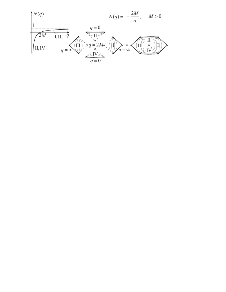
Figure 5: Construction of the Carter–Penrose diagram for the Schwarzschild solution by the method of conformal blocks.

The dependence of the conformal factor $N$ on $q$ is shown in the figure. It has one simple zero at $q=2M$. Thus the interval $(0,\infty)$ is divided on two intervals $(0,2M)$ and $(2M,\infty)$ where the conformal factor is negative (homogeneous solutions) and positive (static solutions). Two triangular conformal blocks II, IV and two square conformal blocks I, III correspond to intervals $(0,2M)$ and $(2M,\infty)$, respectively. Their unique gluing yields the Carter–Penrose diagram for the Schwarzschild solution and is shown in Fig.5. The rules for construction of conformal blocks, their gluing procedure, and the proof of the differentiability of the metric on the glued boundaries are given in [4].

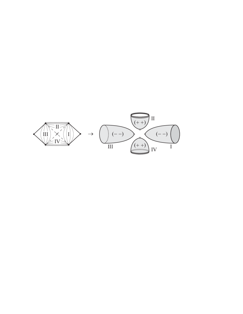
Figure 6: The Carter–Penrose diagram for the Schwarzschild solution in the Euclidean case breaks into four disconnected between themselves surfaces. There are two surfaces I, III with negative definite metric and two surfaces II, IV with positive definite metric corresponding to the regions outside and inside the horizon, respectively.

The Carter–Penrose diagram after changing the signature from Lorentzian to Euclidean breaks into four disconnected between themselves surfaces which are shown in Fig.6. Two Riemannian surfaces I and III with negative definite metric correspond to the region outside the black hole. For these surfaces the total metric has the signature ${\sf\,sign\,}g_{\mu\nu}=(----)$. Negative definiteness of the metric is due to the choice of the signature for the Schwarzschild solution (37) and can be easily changed. This solution is usually considered as the Euclidean version of the Schwarzschild solution. Two surfaces II and IV with positive definite metric correspond to regions inside the horizon of the black hole. The signature of the total metric is ${\sf\,sign\,}g_{\mu\nu}=(++--)$. This spherically symmetric solution is usually considered as unphysical though there is no mathematical reason to discard it.

6 Conclusion

We formulated the method of construction of global (maximally extended) surfaces for a large class of two-dimensional Riemannian metrics having one Killing vector. The smoothness of surfaces and differentiability of metrics are proved. This method is the counterpart of the method of conformal blocks for metrics with Lorentzian signature. Almost anytime each conformal block is the universal covering space for the maximally extended surface. The exceptions are surfaces with a horizon which is a point in the Euclidean case. If there is no conical singularity at this point then the universal covering space appears after the necessary identification of some points of the conformal block.

The transformation from Euclidean signature of the metric to Lorentzian one is interesting. If the Lorentzian surface is represented by the Carter–Penrose diagram with horizons corresponding to zeroes of the conformal factor, then, after the rotation to the Euclidean signature, the Carter–Penrose diagram breaks into disconnected surfaces with positive and negative definite metrics. The change in the signature of the Riemannian metric corresponds to crossing the horizon in the Lorentzian case.

Two-dimensional metrics considered in the present paper arise not only in two-dimensional models but also in higher dimensional gravity when solutions depend essentially only on two of the coordinates. The method can be useful in this case as well.

The author is very grateful to Prof. W. Kummer for numerous and fruitful discussions during which the idea of this work was born in the middle of 90-ties.

References

- [1] M. D. Kruskal. Maximal extension of Schwarzschild metric. Phys. Rev., 119(5):1743–1745, 1960.
- [2] Szekeres G. On the singularities of a riemannian manifold // Publ. Mat. Debrecen. 1960. V. 7, N 1–4. P. 285–301.
- [3] B. Carter. Black hole equilibrium states. In C. DeWitt and B. C. DeWitt, editors, Black Holes, pages 58–214, New York, 1973. Gordon & Breach.
- [4] M. O. Katanaev. Global solutions in gravity. Lorentzian signature. Proc. Steklov Inst. Math., 228:158–183, 2000.
- [5] M. O. Katanaev. Complete integrability of two-dimensional gravity with dynamical torsion. J. Math. Phys., 31(4):882–891, 1990.
- [6] M. O. Katanaev. Conformal invariance, extremals, and geodesics in two-dimensional gravity with torsion. J. Math. Phys., 32(9):2483–2496, 1991.
- [7] M. O. Katanaev. All universal coverings of two-dimensional gravity with torsion. J. Math. Phys., 34(2):700–736, 1993.
- [8] I. V. Volovich and M. O. Katanaev. Quantum strings with a dynamical geometry. JETP Lett., 43(5):267–269, 1986.
- [9] M. O. Katanaev and I. V. Volovich. String model with dynamical geometry and torsion. Phys. Lett., 175B(4):413–416, 1986.
- [10] M. O. Katanaev and I. V. Volovich. Two-dimensional gravity with dynamical torsion and strings. Ann. Phys., 197(1):1–32, 1990.
- [11] M. O. Katanaev, W. Kummer, and H. Liebl. Geometric interpretation and classification of global solutions in generalized dilaton gravity. Phys. Rev. D, 53(10):5609–5618, 1996.
- [12] M. O. Katanaev, W. Kummer, and H. Liebl. On the completeness of the black hole singularity in 2d dilaton theories. Nucl. Phys., B486:353–370, 1997.
- [13] M. O. Katanaev, T. Klösch, and W. Kummer. Global properties of warped solutions in general relativity. Ann. Phys., 276:191–222, 1999.
- [14] M. O. Katanaev. Euclidean two-dimensional gravity with torsion. J. Math. Phys., 38(3):946–980, 1997.
- [15] M. O. Katanaev. Effective action for scalar fields in two-dimensional gravity. Ann. Phys., 296(1):1–50, 2002.
- [16] S. Kobayashi and K. Nomizu. Foundations of differential geometry, volume 1, 2. Interscience publishers, New York – London, 1963, 1969.