The Peculiar Phase Structure of Random Graph Bisection

Abstract

The mincut graph bisection problem involves partitioning the $n$ vertices of a graph into disjoint subsets, each containing exactly $n/2$ vertices, while minimizing the number of “cut” edges with an endpoint in each subset. When considered over sparse random graphs, the phase structure of the graph bisection problem displays certain familiar properties, but also some surprises. It is known that when the mean degree is below the critical value of $2\log 2$, the cutsize is zero with high probability. We study how the minimum cutsize increases with mean degree above this critical threshold, finding a new analytical upper bound that improves considerably upon previous bounds. Combined with recent results on expander graphs, our bound suggests the unusual scenario that random graph bisection is replica symmetric up to and beyond the critical threshold, with a replica symmetry breaking transition possibly taking place above the threshold. An intriguing algorithmic consequence is that although the problem is NP-hard, we can find near-optimal cutsizes (whose ratio to the optimal value approaches 1 asymptotically) in polynomial time for typical instances near the phase transition.

1 Introduction

The graph bisection problem arises in a wide range of contexts, ranging from VLSI design [1] to computer vision [9, 23] to protecting networks from attack [18]. The basic mincut graph bisection (or graph bipartitioning) problem is defined as follows. Given an undirected, unweighted graph, partition its $n$ nodes into two disjoint subsets of equal size, while minimizing the number $w$ of “cut” edges with an endpoint in each subset. This is an NP-hard optimization problem [14].

From a statistical physics perspective, graph bisection is also equivalent to finding the ground state of a ferromagnet constrained to have zero magnetization [13, 22, 27, 24, 25]. Over the past decade, the study of combinatorial optimization problems within the physics community as well as the study of statistical physics approaches within the computer science community has led to remarkable successes [32]. By considering optimization problems over appropriately parametrized ensembles of random instances, physicists have developed methods leading both to analytical predictions of global optima and to algorithmic approaches for finding these. One particularly rich source of insight has been the investigation of phase transition behavior: for many combinatorial optimization problems, both the nature of the solution space and the average-case complexity of algorithms solving the problem are closely related to an underlying phase structure.

In this paper, we consider graph bisection over Erdős-Rényi (Bernoulli) random graphs [12] generated from the ${\cal G}_{np}$ ensemble: given $n$ nodes, place an edge between each of the ${n\choose 2}$ pairs of nodes independently with probability $p$. We are interested in the regime of sparse random graphs, where $p$ scales as $1/n$ and so a vertex’s mean degree $p(n-1)$ is some finite $\alpha$. On such graphs, it is known that a phase transition occurs at $\alpha_{c}=2\log 2$ [16, 27, 24, 25, 26]. For $\alpha<\alpha_{c}$, typical graphs can be bisected without cutting any edges: the bisection width $w$ is zero. For $\alpha>\alpha_{c}$, the graph typically contains a connected component (giant component) of size greater than $n/2$ and so a bisection requires cutting edges, giving $w>0$. In other combinatorial optimization problems such as graph coloring or satisfiability, a similar sharp threshold coincides with a rapid escalation of average-case computational complexity [11, 30, 32].

Additionally, for many of these other problems, at some $\alpha_{d}\leq\alpha_{c}$ the solution space undergoes a structural transition that corresponds to replica symmetry breaking [4, 29]. Define two optimal solutions to be adjacent if the Hamming distance between them is small: an infinitesimal fraction of the variables differ in value. Then below $\alpha_{d}$, any two solutions are connected by a path of adjacent solutions. The solution space may be thought of as a single “cluster”. This is a replica symmetric (RS) phase. But above $\alpha_{d}$, the cluster fragments into multiple non-adjacent clusters, differing by an extensive number of variables. This is a replica symmetry breaking (RSB) phase. In cases where $\alpha_{d}<\alpha_{c}$, such as 3-COL and 3-SAT, this structural transition may contribute to the rise in algorithmic complexity as the main threshold $\alpha_{c}$ is approached from below [28].

We find that the scenario is quite different for graph bisection. Rather than the RSB transition taking place below $\alpha_{c}$, our arguments suggest that it actually occurs somewhere above $\alpha_{c}$. Graph bisection is the first combinatorial optimization problem we are aware of that displays this behavior. Furthermore, in 1987, Liao proposed an analytical solution for bisection width [24, 25] that assumes replica symmetry above $\alpha_{c}$, so our results help validate this prediction. Finally, the same arguments that indicate replica symmetry also suggest an algorithm for finding extremely close approximations to the optimal solution, for $\alpha\in(\alpha_{c},\alpha_{d})$, in polynomial time.

The rest of the paper is organized as follows. In Section 2 we study the bisection width (or “cutsize”) $w$ as a function of mean degree $\alpha$. We present numerical results and derive a new upper bound by analyzing a simple greedy heuristic. In Section 3 we study the solution cluster structure, and argue that the problem is replica symmetric through and beyond the critical threshold $\alpha_{c}=2\log 2$. In Section 4 we conclude with a discussion of the physical and algorithmic consequences of this unusual phase structure.

2 Bisection Width

Formally, the problem is as follows. Given an undirected, unweighted graph $G=(V,E)$ where $|V|=n$ is even, a valid solution is a partition of the vertex set into two disjoint subsets $V_{1}$ and $V_{2}$ such that $|V_{1}|=|V_{2}|=n/2$. An optimal solution is one that minimizes the bisection width $w=|E(V_{1},V_{2})|$, i.e., the number of “cut” edges with an endpoint in each subset. We consider graphs $G$ drawn uniformly at random from ${\cal G}_{np}$, and take our control parameter to be the graph’s mean degree $\alpha=p(n-1)$.

The ${\cal G}_{np}$ ensemble [12, 8] has been studied very extensively since its introduction by Erdős and Rényi in 1959, and many of its structural properties are known. These have a crucial effect on the bisection width.

• For $\alpha<1$, the graph consists only of small components, the largest being asymptotically of size $O(\log n)$. The fraction of monomers, or isolated vertices, is asymptotically almost surely (a.a.s.) itself at least $e^{-1}$. Consequently, with high probability a perfect bisection ($w=0$) exists.

• For $\alpha>1$, there is a unique giant component containing $O(n)$ vertices. The second-largest component is asymptotically of size $O(\log n)$. As long as $\alpha$ is below the threshold $\alpha_{c}=2\log 2$, the giant component a.a.s. contains a fraction $g<1/2$ of the vertices, and the fraction of monomers is still above $1/4$. This allows one to prove [16, 26] that with high probability, $w=0$ for all $\alpha<2\log 2$.

• For $\alpha>2\log 2$, $g>1/2$, and so bisecting the graph requires cutting some of its edges. It is known [26] that $w$ is extensive (scales as $n$) in this regime, as long as $\alpha$ is finite.

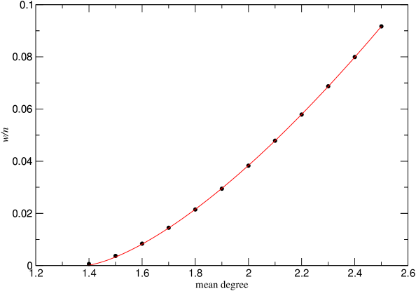
Figure 1: Presumed optimal bisection width, found by extremal optimization on random graphs for $n=2000$. Line shows fit to $\gamma(\alpha-\alpha_{c})^{\beta}$, with $\gamma\approx 0.0783$ and $\beta\approx 1.46$. See also [5].

How does the bisection width constant $w/n$ behave for $\alpha>\alpha_{c}$? Figure 1 shows simulation results using the extremal optimization [6] heuristic to find the presumed optimal bisection. These suggest that the bisection width undergoes a continuous transition at $\alpha_{c}$, and that its first derivative is continuous as well. However, neither of these properties has yet been shown analytically. We will do so now, by deriving a straightforward upper bound on $w$. We give the main elements of the derivation here; a more rigorous mathematical treatment will be provided elsewhere [20].

We obtain the upper bound by “stripping” trees off of the giant component. For random graphs with mean degree $\alpha$, it is known that the fraction $g$ of nodes that are in the giant component is given a.a.s. by [12]

$$g=1-e^{-\alpha g}$$ (1)

and the fraction $b$ of nodes that are in trees within the giant component (the mantle [33]) is a.a.s.

$$b=\alpha g(1-g).$$ (2)

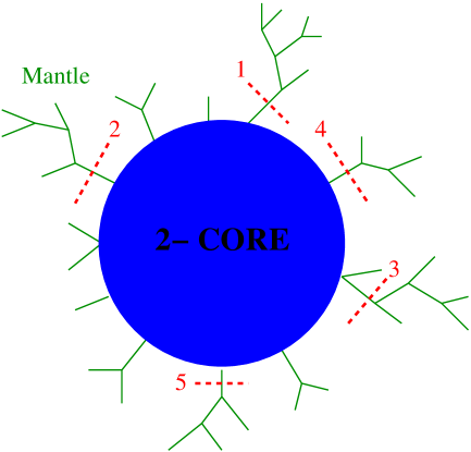
Figure 2: Schematic of giant component consisting of a mantle of trees and a remaining 2-core. Greedy upper bound algorithm cuts trees of decreasing size. Numbers show order of cuts, depicted by dashed lines.

Now imagine a greedy process (Figure 2) of removing trees, starting from the largest one and decreasing in size, until the giant component has been pruned to size $\leq n/2$. In order to know how many trees need to be removed, consider the distribution of tree sizes, $P(t)$. A fortunate consequence of the probabilistic independence in ${\cal G}_{np}$ is that $P(t)$ is simply given by the number of ways of constructing a tree of size $t$ from $q$ roots and $r$ other nodes, where $q=(g-b+\sigma(n))n$ is the number of nodes in the 2-core of the giant component (all nodes not in the mantle) and $r=(b+\tau(n))n$ is the number of nodes in the mantle, with $\sigma(n)$ and $\tau(n)$ being random functions that go a.a.s. to zero [21, 2]. A basic combinatorial argument then gives

$$P(t)={r\choose t}t^{t}\frac{q}{r}\frac{(q+r-t)^{r-t+1}}{(q+r)^{r-1}},$$ (3)

and for large $n$, letting $\rho=b/g$,

$$P(t)\approx\frac{(\rho t)^{t}e^{-\rho t}}{t!}\frac{1-\rho}{\rho}$$ (4)

for $t\geq 1$.

Let $z$ be the total number of trees. Then, given $P(t)$, the total number of nodes in all trees is $\sum_{t=1}^{\infty}tP(t)z$. As this is simply the size of the mantle, it holds a.a.s. that

$$\frac{z}{n}=\frac{b}{\sum_{t=1}^{\infty}tP(t)}.$$ (5)

Let us evaluate this expression. From normalization of $P(t)$,

$$\sum_{t=1}^{\infty}\frac{(\rho t)^{t}e^{-\rho t}}{t!}=\frac{\rho}{1-\rho},$$ (6)

and differentiating with respect to $\rho$,

$$\left(\frac{1}{\rho}-1\right)\sum_{t=1}^{\infty}\frac{(\rho t)^{t}e^{-\rho t}}{(t-1)!}=\frac{1}{(1-\rho)^{2}}.$$ (7)

The left-hand expression is simply $\sum_{t=1}^{\infty}tP(t)$, so Eq. (5) becomes

$$\frac{z}{n}=b(1-\rho)^{2}.$$ (8)

We now wish to set $t_{0}$ so that the number of nodes living on trees of size $\geq t_{0}$ is just barely enough to cover the “excess” of the giant component, $\delta=g-1/2$. In that case, $t_{0}$ satisfies the property

$$\delta > \frac{z}{n}\sum_{t=t_{0}+1}^{\infty}tP(t)$$ (9)

$$= \frac{z}{n}\sum_{t=t_{0}+1}^{\infty}\frac{(\rho t)^{t}e^{-\rho t}}{(t-1)!}\frac{1-\rho}{\rho}$$ (10)

$$= \rho e^{-\rho}\frac{z}{n}\sum_{t=t_{0}}^{\infty}\frac{(t+1)^{t+1}}{t^{t}}\frac{(\rho t)^{t}e^{-\rho t}}{t!}\frac{1-\rho}{\rho}$$ (11)

$$> \rho e^{-\rho}\frac{z}{n}\sum_{t=t_{0}}^{\infty}2(t_{0}+1)P(t)$$ (12)

Given $t_{0}$ satisfying both this and the corresponding lower bound on $\delta$, bisecting the graph is simply a matter of cutting each tree of size $\geq t_{0}$. Any resulting imbalance in the partitions (from “overstripping”) can easily be corrected by transferring enough monomers: there is an extensive number of these, whereas the largest trees are only of size $O(\log n)$. Thus,

$$\frac{w}{n} \leq \frac{z}{n}\sum_{t=t_{0}}^{\infty}P(t)$$ (13)

$$< \frac{\delta(\rho e^{-\rho})^{-1}}{2(t_{0}+1)}$$ (14)

from Eq. (12). In order for the tree-stripping procedure to work, the mantle must contain enough vertices to strip, and so we know that $b\geq\delta$. One can solve Eqs. (1) and (2) numerically to find that this imposes the condition $g<c_{0}$ with constant $c_{0}\approx 0.813$, corresponding to $\alpha\lesssim 2.06$. For $\alpha_{c}\leq\alpha<2.06$, it is straightforward to confirm that $\delta(\rho e^{-\rho})^{-1}<\alpha-\alpha_{c}$, giving

$$\frac{w}{n}<\frac{\alpha-\alpha_{c}}{2(t_{0}+1)}.$$ (15)

Finally, we bound $t_{0}$ itself. A version of Stirling’s formula gives the inequality $t!<t^{t}e^{-t}\sqrt{2\pi t}/(1-1/2t)$, which we apply in Eq. (10):

$$\delta > \frac{z}{n}\sum_{t=t_{0}+1}^{\infty}\frac{t(\rho t)^{t}e^{-\rho t}}{t!}\frac{1-\rho}{\rho}$$ (16)

$$> \frac{b(1-\rho)^{3}}{\sqrt{2\pi}\rho}\sum_{t=t_{0}+1}^{\infty}\frac{\sqrt{t}(1-1/2t)\rho^{t}e^{-\rho t}}{e^{-t}}$$ (17)

$$> \frac{b(1-\rho)^{3}}{\sqrt{2\pi}\rho}\sum_{t=t_{0}+1}^{\infty}(\rho e^{1-\rho})^{t}$$ (18)

$$= \frac{b(1-\rho)^{3}}{\sqrt{2\pi}\rho}\frac{(\rho e^{1-\rho})^{t_{0}+1}}{1-\rho e^{1-\rho}}.$$ (19)

We have just seen that $\alpha-\alpha_{c}>\delta(\rho e^{-\rho})^{-1}$ in the regime of interest, so

$$\alpha-\alpha_{c}>\frac{b(1-\rho)^{3}}{\sqrt{2\pi}\rho^{2}e^{-\rho}(1-\rho e^{1-\rho})}(\rho e^{1-\rho})^{t_{0}+1}.$$ (20)

Then letting $\epsilon=\alpha-\alpha_{c}$,

$$t_{0}+1>\frac{\log(1/\epsilon)+\log\frac{b(1-\rho)^{3}}{\sqrt{2\pi}\rho^{2}e^{-\rho}(1-\rho e^{1-\rho})}}{\log(1/\rho e^{1-\rho})}.$$ (21)

It can be verified that the second term in the numerator is monotone increasing in $g$ and is thus bounded below by its value at $g=1/2$ (the smallest possible giant component size for $\alpha\geq\alpha_{c}$), which corresponds to $\rho=\log 2$. This gives

$$t_{0}+1>\frac{\log(1/\epsilon)-c_{1}}{\log(1/\rho e^{1-\rho})}$$ (22)

where

$$c_{1}=-\log\frac{(1-\log 2)^{3}}{\sqrt{2\pi}\log 2(1-e\log 2/2)}\approx 1.25.$$ (23)

Finally, the denominator in Eq. (22) is also monotone increasing in $g$, and thus bounded above by its value where the mantle is exhausted at $g=c_{0}\approx 0.813$, which corresponds to $\rho=1-1/2c_{0}$. Therefore,

$$t_{0}+1>\frac{\log(1/\epsilon)-c_{1}}{c_{2}}$$ (24)

where

$$c_{2}=-\frac{1}{2c_{0}}-\log\Bigl{(}1-\frac{1}{2c_{0}}\Bigr{)}\approx 0.339.$$ (25)

Inserting this $t_{0}$ bound into Eq. (15) gives the bisection width bound

$$\frac{w}{n}<\frac{c_{2}}{2}\frac{\epsilon}{\log(1/\epsilon)-c_{1}}.$$ (26)

We stress several points regarding this bound. First of all, the result closes the gap between upper and lower bounds on $w/n$ at $\alpha=\alpha_{c}$. The unsurprising fact that both bounds go to zero and the bisection width is continuous at the transition is already apparent from Eq. (14). The less obvious property that its first derivative (with respect to $\alpha$) is also continuous at the transition follows from Eq. (26). Second of all, the denominator of Eq. (26) is only positive for $0<\epsilon<1/e^{c_{1}}$. Numerically, this is roughly $1.39<\alpha<1.67$, which covers a significant fraction of the regime of interest $1.39<\alpha<2.06$. Finally, from Eq. (24) it is clear that $t_{0}$ diverges at the transition, and for sufficiently small $\epsilon$ it satisfies the even simpler bound $t_{0}>\log(1/\epsilon)$. These facts will be significant for the arguments in the next section.

3 Solution Cluster Structure

We now consider the geometry of the solution space for random graph bisection. For a graph $G\in{\cal G}_{np}$, given two distinct optimal bisections $A$ and $B$, define the relative Hamming distance $\mu(A,B)$ to be the fraction of nodes that are in one of the subsets ($V_{1}$ or $V_{2}$) in solution $A$ but in the opposite subset in solution $B$. Since there is a global symmetry under exchange of $V_{1}$ and $V_{2}$, we are interested in $d(A,B)=\min(\mu(A,B),1-\mu(A,B))$.

Define $A$ and $B$ to be $r$-adjacent if $d(A,B)\leq r$. For some small $r$, any two solutions that are connected by a chain of $r$-adjacent solutions are said to be in the same solution cluster. Asymptotically, for a given mean degree $\alpha$, we would like to know what the limiting cluster structure is when $r$ becomes an arbitrarily small constant. One scenario that is common for sufficiently underconstrained combinatorial optimization problems is replica symmetry: for any finite $r>0$, all solutions are with high probability within a single cluster. Another scenario, common for more constrained instances, is one-step replica symmetry breaking: for sufficiently small $r$, there is a large number of disconnected clusters, separated from each other by at least some finite relative Hamming distance.

In what follows, if solutions constructed in a particular way are with high probability $r$-adjacent for any finite $r>0$, we will refer to them as being simply adjacent.

3.1 $\alpha<2\log 2$

Consider graphs where optimal bisections require no cuts in the giant component. We first argue that we can almost surely create such a bisection by populating one of the two subsets only with the largest component and with monomers and dimers (components of size 2). We then use arguments in [19] to show that having created a bisection in this way, it must be in the same cluster as all optimal bisections.

As discussed in Section 2, in ${\cal G}_{np}$ graphs for large $n$, a fraction $e^{-\alpha}$ of nodes are monomers. What about dimers? For a pair of nodes to be a dimer, it must contain an edge (probability $p\approx\alpha/n$), and all other pairs involving one of its two endpoints ($2n-4$ of these) must not contain an edge (probability $1-p$): asymptotically, this occurs with probability $\alpha e^{-2\alpha}/n$. So the expected number of dimer pairs is $\approx\alpha e^{-2\alpha}n/2$, and a.a.s. the fraction of nodes in dimers is $\alpha e^{-2\alpha}$. Thus, a.a.s. the fraction of nodes in monomers or dimers is $s=e^{-\alpha}(1+\alpha e^{-\alpha})$.

For $\alpha\leq 1$, $s>1/2$. For $1<\alpha<2\log 2$, $s$ falls below $1/2$, but one may verify that $g+s>1/2$ where $g$ is the size of the giant component given in Eq. (1). Therefore, as long as $\alpha<2\log 2$, we a.a.s. surely have enough monomers and dimers to fill up a subset that otherwise contains only the largest component (or one of them, if not unique). Call such optimal solutions clean bisections.

Next, we show that any two distinct clean bisections $A$ and $B$ (and hence all clean bisections) must be in the same solution cluster. If the largest component is unique, $A$ and $B$ can differ at most by the choice of which monomers and dimers are selected to be in its subset. If the largest component is not unique, it cannot be a giant component, so two clean bisections can then differ at most by: 1) a component consisting of a vanishing fraction of nodes, and 2) monomers and dimers. In both cases, we can take any one of the differing components in $A$ and swap it with monomers and dimers from the other subset, producing an adjacent clean bisection. By iterating the process, we will necessarily arrive at $B$ through a chain of adjacent clean bisections, since we have already shown that there is a sufficient supply of monomers and dimers for this purpose.

Finally, it is straightforward to see that any optimal solution must be in the same cluster as some clean bisection. This holds for almost the same reason as in the previous paragraph. If the subset containing the largest component also contains any components other than monomers and dimers, each of these asymptotically consists of a vanishing fraction of nodes. They may be iteratively swapped with monomers and dimers to produce a chain of adjacent solutions, leading to a clean bisection.

Since all clean bisections are in the same cluster, and any solution is in the same cluster as some clean bisection, all solutions must lie within a single cluster for $\alpha<2\log 2$. This is a replica symmetric phase.

3.2 $\alpha\geq 2\log 2$

When the bisection width is nonzero, the situation is more complicated. Now we must consider the different ways in which optimal bisections can cut the giant component. We will show that up to some $\alpha_{d}>\alpha_{c}$, optimal bisections avoid a central core of the giant component and are restricted to a well-defined periphery. We then give arguments suggesting that for those graphs, all optimal bisections are in a single cluster.

3.2.1 The expander core

Call the giant component $S$, and imagine that for any $\alpha\geq 2\log 2$, some identifiable part of it, $X\subseteq S$, is an expander. This means that cutting off any piece $X_{0}$ from $X$ requires (asymptotically) at least some finite expansion

$$h=\frac{|E(X\setminus X_{0},X_{0})|}{\min(|X\setminus X_{0}|,|X_{0}|)},$$ (27)

i.e., the number of cut edges per vertex in the broken piece. The expander $X$ would then be precisely the central core that optimal bisections avoid, for $\epsilon=\alpha-\alpha_{c}$ less than some constant. The reason is as follows. We have seen in Section 2 that when cutting trees only, the smallest tree needed is of size

$$t_{0}>\log(1/\epsilon),$$ (28)

and so the largest expansion is

$$h<\frac{1}{\log(1/\epsilon)}.$$ (29)

For sufficiently small $\epsilon$, this must fall below the (finite) value of $h$ for the expander. Thus, below some finite $\epsilon_{0}>0$, trimming the giant component’s excess requires fewer cuts if these are performed exclusively within the mantle than if any part of the cuts are performed within the core.

One might hope that the 2-core is an expander, in which case greedily trimming trees would in fact be the optimal way to bisect a graph. As it happens, this is almost certain not true. Consider the 2-core’s spectral gap, the difference $\lambda_{1}-\lambda_{2}$ between the two largest eigenvalues of its connectivity matrix. Via Cheeger’s inequality [10], this yields an upper bound on expansion. Figure 3 suggests that the spectral gap likely vanishes (albeit slowly) as $n\to\infty$, implying that the 2-core’s expansion vanishes, presumably due to the existence of cycles of length $\sim\log n$. Certain “bottlenecks” in the 2-core could then provide more efficient cuts than trees in the mantle.

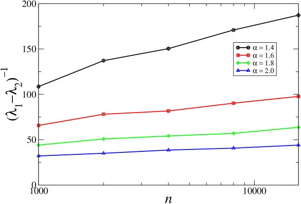
Figure 3: Reciprocal of spectral gap. For mean degree $\alpha=1.4$ through $\alpha=2.0$, on graphs of size $n=1000$ up to $n=16000$ this quantity vanishes roughly as $\sim 1/\log n$.

But some further intuition comes from considering random cuts in the 2-core. Figure 4 shows the minimum expansion from a number of ways of randomly slicing the 2-core into two pieces. These numerical results, which we originally reported in [17], suggest that for large $n$ the minimum expansion never falls below a constant. This means that any bottlenecks that do exist in the 2-core are not immediately apparent, and some significant part of the 2-core could in fact be an expander.

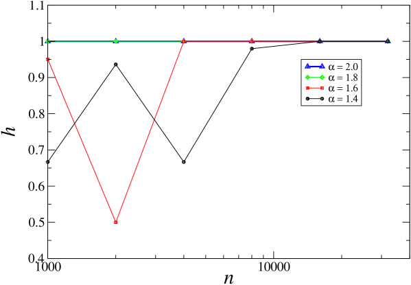
Figure 4: Smallest expansion over a random sample of ways of slicing the 2-core into two pieces. Randomly chosen nodes are sequentially separated from the 2-core until half of the 2-core has been cut. For each value of mean degree $\alpha$, and for each size from $n=1000$ to $n=32000$, this random sequence is repeated 10 times on each of 100 graphs. Results show the lowest expansion value found over the course of all 10 sequences and over all 100 graphs. For increasing graph sizes, this value approaches 1.

Subsequent results by Benjamini et al. [2] have confirmed that this is indeed the case: for all $\alpha>1$, they give an explicit procedure for stripping the giant component down to an expander core. The giant component is a “decorated expander,” with many small ($O(\log n)$ at the largest) “decorations” $D_{i}$ attached to the expander core $X$, as shown schematically in Figure 5. Therefore, by our previous argument, below some finite $\epsilon_{0}$, the cuts in all optimal bisections are restricted to the decorations $D_{i}$.

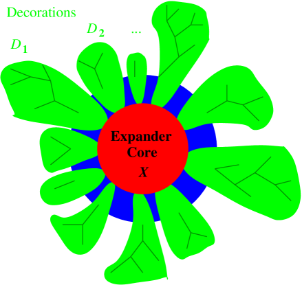
Figure 5: A different view of the giant component in Figure 2, shown here as an identifiable expander core $X$ within the 2-core. The trees are now contained within numerous small decorations $D_{i}$ that are attached to the expander core.

3.2.2 Consequences for solution structure

We now use arguments related to the ones in Section 3.1 to suggest that for $\epsilon<\epsilon_{0}$ ($\alpha<\alpha_{d}=2\log 2+\epsilon_{0}$), all optimal solutions are contained within a single cluster. We first show how to construct a neat bisection. By neat, we mean that one of the two subsets contains only the expander core, some attached decorations, and monomers. We then present arguments suggesting that this bisection, even if not optimal, is adjacent to a neat optimal bisection that is in the same cluster as all optimal bisections, thus replica symmetry holds for all $\alpha<\alpha_{d}$.

The construction procedure is as follows. Consider the giant component $S$ as being composed of the expander core $X$ and decorations $D_{i}$ as in Figure 5. These are disjoint subsets, with some edges connecting the $D_{i}$ to $X$ but none connecting the $D_{i}$ to each other [2]. For each decoration $D_{i}$, find the nonempty subset $D_{i}^{1}\subseteq D_{i}$ that minimizes the expansion

$$h_{i}^{1}=\frac{|E(S\setminus D_{i}^{1},D_{i}^{1})|}{|D_{i}^{1}|}$$ (30)

resulting from cutting off the piece $D_{i}^{1}$. The value of $h_{i}^{1}$ may be interpreted as a “cost” per node that we attribute to each node in $D_{i}^{1}$. Now repeat this procedure on $D_{i}\setminus D_{i}^{1}$, resulting in a new piece $D_{i}^{2}$, except that this time we find the $D_{i}^{2}$ minimizing the marginal cost of cutting off $D_{i}^{2}$ given that $D_{i}^{1}$ is already cut off, i.e.,

$$h_{i}^{2}=\frac{|E(S\setminus(D_{i}^{1}\cup D_{i}^{2}),D_{i}^{1}\cup D_{i}^{2})|-|E(S\setminus D_{i}^{1},D_{i}^{1})|}{|D_{i}^{2}|}.$$ (31)

Recursively perform the procedure, letting

$$h_{i}^{j}=\frac{|E(S\setminus\bigcup_{l=1}^{j}D_{i}^{l},\bigcup_{l=1}^{j}D_{i}^{l})|-h_{i}^{j-1}|D_{i}^{j-1}|}{|D_{i}^{j}|},$$ (32)

until decoration $D_{i}$ has been completely partitioned into disjoint subsets $D_{i}^{1},\dots,D_{i}^{m}$. It is straightforward to confirm that these, by construction, are now ordered in increasing marginal cost $h_{i}^{1}\leq\dots\leq h_{i}^{m}$, where the total cost $|E(S,D_{i})|$ of cutting the entire decoration is simply equal to the sum of the marginal costs over all nodes,

$$|E(S,D_{i})|=\sum_{j=1}^{m}h_{i}^{j}|D_{i}^{j}|.$$ (33)

Note that $h_{i}^{j}$ is the minimum possible cost of cutting a node in $D_{i}^{j}$. Since cuts in optimal solutions are restricted to decorations, generating a neat optimal bisection requires an aggregated ranking of all subsets of all decorations, $D_{i}^{j}$, according to their costs $h_{i}^{j}$. Analogously to the greedy algorithm in Section 2, where we stripped trees in increasing order of expansion, we now strip the pieces of the decorations until the giant component’s excess has been removed. As with the greedy algorithm, this can result in overstripping. There may also be numerous pieces with an equal ranking, leaving the choice of which ones to pick in order to overstrip as little as possible. But due to the maximal size of the decorations [2], the largest of these pieces is $O(\log n)$. So regardless of which we choose, as with tree-stripping, we can compensate for the imbalance by transferring some of the extensive supply of monomers. The result is a neat bisection, albeit not necessarily an optimal one.

In principle, by perfectly selecting the final pieces of equal rank and thereby minimizing the cost of overstripping, we can even form any neat optimal bisection in this way. We discuss this in the next section. But no matter how we select the final pieces, it seems highly likely that our construction gives a solution differing from some optimal one by at most the number of variables contained in a finite number of these pieces, which is $O(\log n)$. Furthermore, it is not difficult to see that all neat (not necessarily optimal) bisections that use the identical choice of compensating monomers lie within a single cluster. It then follows that among these neat bisections, all those that are optimal are in a single cluster as well. And every neat optimal bisection must then be in the same cluster, since successively swapping monomers gives a chain of adjacent solutions connecting them.

Finally, for similar reasons as in Section 2, any optimal bisection must be in the same cluster as some neat optimal bisection. If the subset containing the expander core also contains components other than monomers, each one can have size at most $O(\log n)$ and can be swapped with monomers from the other subset to produce an adjacent optimal bisection. Iterating this process leads to a neat optimal bisection. Consequently, the argument implies that for $2\log 2<\alpha<\alpha_{d}$, all optimal bisections lie within a single cluster, and the replica symmetric phase extends up to $\alpha_{d}>\alpha_{c}$.

Above $\alpha_{d}$, the solution structure is less clear. When $\alpha$ is large enough, optimal cuts are no longer necessarily restricted to the decorations: the expander core likely needs to be cut as well. In that case, the sizes of the cut pieces could well be extensive. One could easily imagine extensive gaps in the solution structure, leading to multiple clusters and replica symmetry breaking. Although we have no direct evidence of it, we speculate that this is the case for $\alpha$ greater than some finite value, suggesting an RSB phase boundary at or above $\alpha_{d}$, i.e., above the critical threshold $\alpha_{c}$.

4 Discussion and Conclusions

Our study points to an unusual kind of phase structure for random graph bisection. The typical scenario, in random combinatorial optimization problems displaying a sharp threshold in the objective function’s behavior, is that an RSB transition takes place at or below the main critical threshold: $\alpha_{d}\leq\alpha_{c}$. By contrast, graph bisection appears to be replica symmetric up to and beyond the threshold, with $\alpha_{d}>\alpha_{c}$. We note that this lends support to an analytical bisection width prediction proposed by Liao in 1987 [24, 25]. Let us now comment on several further aspects of $\alpha_{d}$, as well as on the intriguing algorithmic consequences of this phase picture.

Although $\alpha_{d}$ is strictly greater than $\alpha_{c}$, it may not be much greater. As mentioned at the end of Section 2, our bisection width bound is only valid for $\alpha<1.67$. That bound is needed for being able to restrict optimal cuts to the giant component’s decorations. We do not presently have any other quantitative bound or estimate on the specific value of $\alpha_{d}$. However, some further qualitative observations come from examining the procedure for obtaining the expander core. Roughly speaking, Benjamini et al. [2] strip the giant component down to what we call a 2.k-core, namely a connected subgraph of the giant component where all vertices have degree at least 2 (no trees) and where the largest chain is of length $k$. The $2.k$-core is an expander as long as $k$ is a sufficiently large finite constant. The construction of [2] does not explicitly state how large $k$ must be, or what the minimum expansion value $h$ is for the $2.k$-core at a given mean degree $\alpha$. But decreasing values of $k$ clearly result in smaller $2.k$-cores (Figure 6), and presumably in larger expansion as more long chains are removed. This would lead to a higher $\alpha_{d}$. Thus, by picking the smallest possible $k$ (for every $\alpha$) that still yields an expander core, the resulting expansion gives, via Eq. (29), the largest possible $\alpha_{d}$ for which we can be sure that graph bisection is replica symmetric at all $\alpha<\alpha_{d}$.

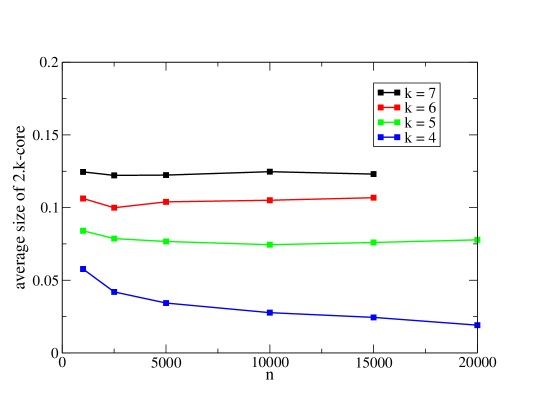
Figure 6: Fraction of nodes in the $2.k$-core, $k=4$ through $k=7$, at $\alpha=1.4$. Numerical results are averaged over 200 instances, for increasing values of $n$.

Algorithmically, the striking consequence of our study is that we may obtain near-optimal bisections and perhaps even optimal ones, for all $\alpha<\alpha_{d}$, in polynomial time. By near-optimal, we mean that the ratio of its bisection width to the optimal value approaches 1 asymptotically. We do this by stripping the giant component down to the expander core (using any sufficiently large $k$), and then following the construction in Section 3.2.2. The stripping process and decoration identification [2] takes polynomial time. The next subtlety is breaking a decoration $D_{i}$ into the correct disjoint pieces $D_{i}^{j}$: an exhaustive approach to finding $D_{i}^{1}$ involves comparing all of the $2^{|D_{i}|}$ ways of partitioning $D_{i}$ into two subsets. But since no decoration $D_{i}$ has more than $O(\log n)$ nodes, this can be done in $n^{O(1)}$ steps, and then all pieces $D_{i}^{j}$ can be found and ranked ($h_{i}^{1}\leq\dots\leq h_{i}^{m}$) in $n^{O(1)}$ steps. For the final pieces of equal rank, even if we simply pick them in arbitrary order we will overstrip by at most $O(\log n)$. Thus, in polynomial time we reach a solution whose (extensive) bisection width is within $O(\log n)$ of the optimal one.

Of course, the $O(1)$ constant in the exponent may be quite large, which could make this result largely a theoretical one. But it is worth noting that we have some freedom to decrease the size of the decorations, and thus lower the constant. If, say, instead of using the smallest possible $k$ that gives an expander core, we use the largest possible $k$ that gives expansion greater than our tree-cutting bound (Eq. (29)), this will strip the minimum possible from the giant component. In this way, we may be able to minimize the size of the largest decoration.

It would be particularly remarkable if some version of our construction could give a true optimal bisection, with high probability, in polynomial time. For this, we need to pick the final pieces of equal rank so as to minimize overstripping. The difficulty is that the number of such pieces is likely to be infinite: an extensive number of nodes is contained collectively within the decorations, while there are at most $O(\log^{2}n)$ possible marginal costs ($O(\log n)$ possible integers for the numerator and $O(\log n)$ possible integers for the denominator). On the other hand, it could well be that of the infinite number of final pieces, a finite fraction of them have any given finite size $|D_{i}^{j}|$. In that case, a simple greedy procedure will find a collection of pieces that minimizes overstripping. Having minimized overstripping, one still needs to check whether it is possible to lower the bisection width further by restoring a small fragment of a cut piece. If the amount we overstrip is $O(\log n)$, then exhaustively checking this could require $\sim{n\choose\log n}$ steps. But more likely, one can strengthen our analysis to show that the final pieces are in fact of size $O(1)$, in which case the last operation could also be accomplished in polynomial time. Clearly, this intuition is far from a proof of any sort. But if indeed the optimal bisection can be found in polynomial time for $\alpha<\alpha_{d}$, we would have a very unusual example of an NP-hard optimization problem whose typical-case complexity is polynomial at and above the main threshold $\alpha_{c}$.

We offer two final remarks about other versions of the problem. First, our approach suggests that the peculiarities of random graph bisection’s phase structure are closely related to the problem’s global constraint — the fact that a subset cannot be larger than $n/2$ — combined with the specific topology of the giant component in ${\cal G}_{np}$. This means that the problem of balanced multiway graph partitioning on ${\cal G}_{np}$ graphs should have very similar characteristics, and can likely be analyzed through similar means. Second, the situation is very different if instead of ${\cal G}_{np}$ we use a graph ensemble that has local geometric structure. An example is the random geometric graph ensemble ${\cal G}_{nr}$ [31], where nodes are placed uniformly at random in a unit square and pairs are connected by an edge if separated by distance $\leq r$. In this case, the giant component is very unlikely to have any expander core due to its large diameter. Rather than having a tree-like periphery, it contains numerous local cliques, and minimizing the bisection width involves locating the bottlenecks in between those cliques. But at the same time, ${\cal G}_{nr}$ graphs have useful lattice-like properties [15], with the optimal bisection width scaling [31, 7] as $w\sim\sqrt{n}$, precisely as one finds on a regular 2-dimensional lattice structure. We expect that the structure of bisections is closely related to the geometry of the giant component in bond percolation on a lattice, which has been studied [3]. Adapting that analysis could lead to nontrivial bounds on $w$ and rapid algorithms finding very close approximations to the optimal cut in ${\cal G}_{nr}$.

5 Acknowledgments

This work was supported by the U.S. Department of Energy at Los Alamos National Laboratory under contract DE-AC52-06NA25396 through the Laboratory Directed Research and Development Program, a Marie Curie International Reintegration Grant within the 6th European Community Framework Programme, a PN II/Parteneriate grant from the Romanian CNCSIS, and a National Science Foundation grant DMR-0312510.

References

- [1] C. J. Alpert and A. B. Kahng. Recent directions in netlist partitioning: a survey. Integration, the VLSI Journal, 19:1–81, 1995.
- [2] I. Benjamini, G. Kozma, and N. Wormald. The mixing time of the giant component of a random graph. arXiv:math.PR/0610459, 2006.
- [3] I. Benjamini and E. Mossel. On the mixing time of a simple random walk on the supercritical percolation cluster. Probability Theory and Related Fields, 125:408–420, 2003.
- [4] G. Biroli, R. Monasson, and M. Weigt. A variational description of the ground state structure in random satisfiability problems. European Physical Journal B, 14:551–568, 2000.
- [5] S. Boettcher. Extremal optimization of graph partitioning at the percolation threshold. Journal of Physics A: Mathematical and General, 32:5201–5211, 1999.
- [6] S. Boettcher and A. G. Percus. Nature’s way of optimizing. Artifical Intelligence, 119:275–286, 2000.
- [7] S. Boettcher and A. G. Percus. Extremal optimization for graph partitioning. Physical Review E, 64:026114, 2001.
- [8] B. Bollobas. Random Graphs. Cambridge University Press, Cambridge, UK, 2001.
- [9] Y. Boykov, O. Veksler, and R. Zabih. Fast approximate energy minimization via graph cuts. IEEE Transactions on Pattern Analysis and Machine Intelligence, 23:1222–1239, 2001.
- [10] J. Cheeger. A lower bound for the smallest eigenvalue of the Laplacian. In Problems in analysis (Papers dedicated to Salomon Bochner, 1969), pages 195–199. Princeton Univ. Press, Princeton, N. J., 1970.
- [11] P. Cheeseman, B. Kanefsky, and W. F. Taylor. Where the really hard problems are. In Proceedings of the 12th International Joint Conference on Artificial Intelligence (IJCAI’91), pages 331–337, San Mateo, CA, 1991. Morgan Kaufmann.
- [12] P. Erdős and A. Rényi. On random graphs. Publ. Math. Inst. Hungar. Acad. Sci., 1959.
- [13] Y. Fu and P. Anderson. Application of statistical mechanics to np-complete problems in combinatorial optimisation. Journal of Physics A: Mathematical and General, 19(9):1605–1620, 1986.
- [14] M. R. Garey and D. S. Johnson. Computers and Intractability. W.H. Freeman, New York, 1979.
- [15] A. Goel, S. Rai, and B. Krishnamachari. Monotone properties of random geometric graphs have sharp thresholds. Annals of Applied Probability, 15:2535–2552, 2005.
- [16] M. Goldberg and J. Lynch. Lower and upper bounds for the bisection width of a random graph. Congr Numer, 49, 1985.
- [17] B. Gonçalves, G. Istrate, A. Percus, and S. Boettcher. The core peeling algorithm for graph bisection: an experimental evaluation. Technical Report LA-UR 06-6863, Los Alamos National Laboratory, 2006.
- [18] P. Holme, B. J. Kim, C. N. Yoon, and S. K. Han. Attack vulnerability of complex networks. Phys. Rev. E, 65:056109, 2002.
- [19] G. Istrate, S. Kasiviswanathan, and A. Percus. The cluster structure of minimum bisections of sparse random graphs. Technical Report LA-UR 06-6566, Los Alamos National Laboratory, 2006.
- [20] G. Istrate, S. Kasiviswanathan, and A. G. Percus. The bisection width and solution cluster structure of sparse random graphs. In preparation.
- [21] S. Janson, T. Łuczak, and A. Ruciński. Random Graphs. John Wiley & Sons, Inc., New York, 2000.
- [22] I. Kanter and H. Sompolinsky. Mean-field theory of spin-glasses with finite coordination number. Physical Review Letters, 58(2):164–167, 1987.
- [23] V. Kolmogorov and R. Zabih. What energy functions can be minimized via graph cuts? IEEE Transactions on Pattern Analysis and Machine Intelligence, 26:147–169, 2004.
- [24] W. Liao. Graph bipartitioning problem. Physical Review Letters, 59(15):1625–1628, 1987.
- [25] W. Liao. Replica-symmetric solution of the graph-bipartitioning problem. Physical Review A, 37(2):587–595, 1988.
- [26] M. J. Łuczak and C. McDiarmid. Bisecting sparse random graphs. Random Struct. Algorithms, 18:31–38, 2001.
- [27] M. Mézard and G. Parisi. Mean-field theory of randomly frustrated systems with finite connectivity. Europhysics Letters, 3(10):1067–1074, 1987.
- [28] M. Mézard, G. Parisi, and R. Zecchina. Analytic and algorithmic solutions of random satisfiability problems. Science, 297:812–815, 2002.
- [29] M. Mézard and R. Zecchina. Random K-satisfiability problem: from an analytical solution to an efficient algorithm. Physical Review E, 66:056126, 2002.
- [30] D. G. Mitchell, B. Selman, and H. J. Levesque. Hard and easy distributions for SAT problems. In P. Rosenbloom and P. Szolovits, editors, Proceedings of the Tenth National Conference on Artificial Intelligence, pages 459–465, Menlo Park, California, 1992. AAAI Press.
- [31] M. D. Penrose. Random Geometric Graphs. Oxford University Press, Oxford, 2003.
- [32] A. G. Percus, G. Istrate, and C. Moore. Computational Complexity and Statistical Physics. Oxford University Press, New York, 2006.
- [33] B. Pittel. On tree census and the giant component in sparse random graphs. Random Struct. Algorithms, 1:311–342, 1990.