A statistical approximation to solve ordinary differential equations

Abstract

We propose a physical analogy between finding the solution of an ordinary differential equation (ODE) and a $N$ particle problem in statistical mechanics. It uses the fact that the solution of an ODE is equivalent to obtain the minimum of a functional. Then, we link these two notions, proposing this functional to be the interaction potential energy or thermodynamic potential of an equivalent particle problem. Therefore, solving this statistical mechanics problem amounts to solve the ODE. If only one solution exists, our method provides the unique solution of the ODE. In case we treat an eigenvalue equation, where infinite solutions exist, we obtain the absolute minimum of the corresponding functional or fundamental mode. As a result, it is possible to establish a general relationship between statistical mechanics and ODEs which allows not only to solve them from a physical perspective but also to obtain all relevant thermodynamical equilibrium variables of that particle system related to the differential equation.

I INTRODUCTION

Ordinary differential equations are one way physicists model physical phenomena. To solve them, a great variety of analytical and numerical methods are available in the literature Hildebrand73 ; Kaplan85 .

Trough this article we wish to solve some problems that arise in vibration theory making an analogy of them with a system of particles, a well known issue treated in Statistical Mechanics. If this analogy is made, all the tools used in Statistical Mechanics are available for tackling these type of problems. For example, one is able to calculate the entropy or the specific heat of the system, something which is, at least, difficult to imagine in a typical vibration problem. From a more general perspective, we extend the same analogy and apply it to find the solutions of ordinary differential equations (ODEs) of general type (see section II).

The general method proposed here could be resumed in the following way. From a mathematical viewpoint, it is possible to obtain the solution of an ODE from the minimization of a functional. On the other hand, a thermodynamic potential is represented by a functional. We connect these two notions, proposing the functional which leads to the solution of an ODE, to be the interaction potential energy or thermodynamic potential of an equivalent particle problem. Therefore, solving this statistical mechanics problem amounts to solve the ODE. For the case where only one solution exists, the method allows to obtain the unique solution of the ODE. Clearly, when we treat vibrational problems, an eigenvalue equation must be solved with infinite possible solutions. This case our method is capable of obtaining the fundamental mode or absolute minimum of the corresponding functional.

The principal aim of our work is to show (a) how the previously proposed correspondence is used to attain the solution of ordinary differential equations, (b) the theoretical basis upon which it is sustained and (c) the way it can be treated within a stochastic framework.

The present work is organized as follows. In section II, we show how the problem of solving a general kind of ODE can be transformed to a problem of minimization of a functional (weak solution of the differential equation Rektorys75 ). Section III presents the foundations of equilibrium statistical analysis viewed as a minimization of a thermodynamic potential. This provides the theoretical the basis of our developed method. Section IV describes the general aspects of the numerical scheme and algorithm implementation. Section V is devoted to find the solution of an ODE employing a stochastic framework. This method allow us to solve the ODE proposing an equivalent Langevin (stochastic) equation. At the end, in section VI, several numerical experiments which will sustain our theoretical hypothesis will be developed and solved. Finally, some conclusions will be outlined.

II MATHEMATICAL PROBLEM

There are many possible approaches to find the solution of ODEs Hildebrand73 ; Kaplan85 . From all of them, we are interested in that one which transforms the problem of finding the solution of an ODE into the minimization of a functional. To do this we must recall some results of functional analysis.

II.1 Obtaining a minimum principle for the differential equation

The most general form of an ODE of order $2k$ can be written as Rektorys75

$$Au(x)=\mathop{\displaystyle\sum}_{i=0}^{k}(-1)^{i}(p_{i}u^{(i)}(x))^{(i)}=f$$ (1)

where $u(x)$ is an element of a Hilbert space $\mathcal{H}_{A}$, $x\in\Re$ and $u^{(i)}(x)$ is the derivative of order $(i)$ of $u(x)$. Also $f\in L_{2}(a,b)$ ($L_{2}(G)$ Hilbert space of functions square integrable in the domain $G$) and $p_{i}(x),i=0,1,...,k$ are functions continuous with their derivatives up to the $i-th$ order inclusive in the closed interval $[a,b]$ which satisfy

$$p_{i}(x)\geq 0\ \text{in}[a,b],\ i=0,1,...,k-1$$ (2)

$$p_{k}(x)\geq p\ \text{in}[a,b],\ p=const.$$ (3)

For the rest of the paper, homogeneous boundary conditions will be considered with no loss of generality.

Then, it is possible to look for the generalized solution $u^{\ast}$ of equation (1) as that element which minimizes the functional

$$F(u)=\mathop{\displaystyle\sum}_{i=0}^{k}\mathop{\displaystyle\int}_{0}^{L}p_{i}(u^{(i)})^{2}dx-2\mathop{\displaystyle\int}_{0}^{L}fudx$$ (4)

in the corresponding Hilbert space $\mathcal{H}_{A}$, where operator $A$ is defined. There exists a requirement of positive definiteness of operator $A$ that ensures that the extreme value of (4) or (5) is the desired solution $u^{\ast}$ of the problem.

For the eigenvalue problem, $Au-\lambda u=0,\ \lambda\in\Re$, the functional to be minimized coincides with the corresponding eigenvalue $\lambda$ and it reduces to

$$F(u)\equiv\lambda=\frac{\mathop{\displaystyle\sum}_{i=1}^{k}\mathop{\displaystyle\int}_{0}^{L}p_{i}(u^{(i)})^{2}dx}{\mathop{\displaystyle\int}_{0}^{L}u^{2}dx}$$ (5)

In this case, infinite minima exist, each of them corresponding to the associated eigenvalues

$$\lambda_{1}\leq\lambda_{2}\leq...$$ (6)

Equation (6) states that the first (or fundamental) eigenvalue $\lambda_{1}$ is the minimum possible eigenvalue and the corresponding eigenfunction is $u_{1}$; i. e. $F(u_{1})$ is the absolute minimum of $F(u)$ Rektorys75 .

Summing up, a differential operator can be transformed into a functional so that minimizing this functional equals to solving the ODE.

III STATISTICAL TREATMENT

As a second step towards attaining the solution of ODEs, we must adequate the problem to be treated as a standard particle problem in statistical mechanics. To this end, we must think on a $n$ particle system in a one dimensional box of size $L$, where a point in the $n$ dimensional configurational phase space can be denoted by $\mathbf{q}=\{q_{1},q_{2},...q_{n}\}$, being $q_{j}$ the position of particle $j$. Now, a link between the representation of this system in configurational phase space $\mathbf{q}$ with the description of possible candidate solutions of the ODE $u(x)$ (see equation 1) is proposed through an adequate discretization of $u(x)$.

III.1 Discretization of $u(x)$

Consider now any possible candidate to the solution of a particular kind of ODE, named $u(x)$. This continuous function is an element in the corresponding Hilbert space $\mathcal{H}_{A},x\in\Re$ where operator $A$ is defined, and belongs to the domain of the functional $F(u)$. The proposed discretization of $u$ will be settled from the consideration of $n$ sites labelled with the discrete index $l$ of a 1 dimensional lattice. Then, the function $u(x)$ is taken as the limit $n\rightarrow\infty$ from the field functions $u_{l}(x_{l})$. So the link between our system of particles and that element $u(x)$ is naturally settled as $u_{l}(x_{l})=q_{l}$. Each $u_{l}$ can take any value between $-\infty$ and $\infty$. A possible configuration of our $n$ particle system is then considered by specifying the value of $u_{l}$ at each site $l$ or simply the lattice vector $\mathbf{q}=\{u_{1}(x_{1}),...,u_{l}(x_{l}),...u_{n}(x_{n})\}$. Through this connection, it is possible to apply the whole statistical framework to treat this equivalent new problem.

III.2 Equilibrium statistical analysis

The next step is to formulate the problem as in standard statistical mechanics. To do this, we will consider our particle system in the canonical ensemble. So far we have made a connection between the domain of the functional $F(u)$ with the microstates of a thermal system, represented by $\mathbf{q}$. With this in mind, and using the expression for the probability density in the canonical ensemble $\rho_{\mathbf{q}}=e^{-\beta H(\mathbf{q})}/Z$, our proposal is to define an equivalent problem, such that the Hamiltonian $H(\mathbf{q})$ is replaced by our functional $F(\mathbf{q})$ i. e.

$$\rho_{\mathbf{q}}=\frac{\exp{(-\beta F(\mathbf{q}))}}{Z}$$ (7)

Here, as well as in standard statistical mechanics $Z$ represents the partition function ( this time $Z=\int e^{-\beta F(\mathbf{q})}d\mathbf{q}$) and $\beta$ can be considered a parameter equivalent to the temperature. Automatically, this probability density maximizes a new “entropy”, and lead us to pose an equivalent state equation:

$$\mathcal{A}=F(\mathbf{q})-ST$$ (8)

Where $\mathcal{A}$ can be thought as the corresponding Helmholtz potential of the equivalent problem. In case of solving the eigenvalue problem in vibration theory, for example, $F(\mathbf{q})$ turns to be Rayleigh’s quotient $R(\mathbf{q})$ Newland06 ; Leissa05 . A briefly mathematical support is given in appendix A which assures the mathematical possibility of the probability density proposed.

Summarizing, since our problem of solving the ODE has been transformed into an equivalent thermal system, all the mathematical framework of Statistical Mechanics could be applied. For the sake of brevity, here we only outline how several typical thermodynamical equilibrium variables such as entropy and specific heat, could be calculated using previous relations. For example, for the specific heat $C(T)$ we have, by definition

$$C(T)=\frac{d\langle F(\mathbf{q})\rangle}{dT}=\frac{[\langle F(\mathbf{q})\rangle^{2}-\langle F(\mathbf{q})^{2}\rangle]}{T^{2}}$$ (9)

where $\langle\rangle$ means equilibrium or ensemble average and could be calculated for each $T$ by Monte-Carlo sampling (see section IV).

Also the entropy could be obtained in the same form applying the well known relation

$$\frac{dS}{dT}=\frac{C(T)}{T}$$ (10)

which integrated, using equation (9), give us

$$S(T)=S(T_{1})-\mathop{\displaystyle\int}_{T_{1}}^{T}\frac{[\langle F(\mathbf{q})\rangle^{2}-\langle F(\mathbf{q})^{2}\rangle]}{T^{\prime 3}}dT^{\prime}$$ (11)

IV PROPOSED ALGORITHM

Having established this new equivalent problem, we apply the whole framework of equilibrium statistical analysis to obtain the extreme value of $F(\mathbf{q})$. Our main tool for solving problems through this paper is based on Metropolis Monte-Carlo algorithm Metro53 . Briefly, this algorithm ensures a way to sample canonical ensemble proposing a transition probability $P_{\mathbf{q^{\prime},q}}$ which satisfies detailed balance. For our case, it takes the form

$$P_{\mathbf{q^{\prime},q}}=\frac{\rho_{\mathbf{q^{\prime}}}}{\rho_{\mathbf{q}}}=\exp\left(-\frac{\Delta F\left(\mathbf{q^{\prime}},\mathbf{q}\right)}{T}\right)$$ (12)

where $T=1/\beta$, $k_{b}\equiv 1$.

With this transition probability, we construct an algorithm that can sample our $n-$dimensional configurational phase space $\mathcal{H}_{n}$, whose limit as $n\rightarrow\infty$ tends to Hilbert space $\mathcal{H}_{A}$. Each equilibrium state, which can be reached by waiting sufficient time (Monte-Carlo steps), is a function of parameter $T$ in which all possible configurations differ from each other in $\pm T$. Obviously, this also means that for a given $T>0$ there exist many equilibrium configurations and only for $T=0$ it reduces to one.

The proposed algorithm takes the previous idea and uses it in the same way as in standard simulated annealing Kirk83 . We’ve just exposed that equilibrium states are governed by parameter $T$. So, if one diminishes its value in a way so as to go through successive equilibrium states, then, the most representative points of the ensemble will be sampled. In the limit as $T\rightarrow 0$, each different configuration will differ from each other in an infinitesimal quantity which means, from the notion of a variation of a functional, that we reach a minimum $\mathbf{q^{\ast}}=u^{\ast}$ (solution of the ODE). By this way, the algorithm is supposed to be capable of avoiding relative minima, providing the absolute minimum of the functional. For the eigenvalue problem, this allows only to obtain the fundamental mode and lowest eigenvalue. However, higher modes which correspond to relative minima, could be obtained in principle if we impose restrictions to the functional, such as symmetry or number of nodes; these topics will be explored in future works.

IV.1 Solution generation

Here, we address the problem of generating candidate solutions $\mathbf{q^{\prime}}$ from an existing one $\mathbf{q}$ (solution generation scheme). To attempt this end, we will first make a brief survey of the calculus of variations Hildebrand73 . The variation of a functional $F(u)=\mathop{\displaystyle\int}f(u,u^{(1)},...,u^{(s)})dx$ which depends on the function $u(x)$ and its derivatives of order $\nu$, $u^{(\nu)}$ is

$$\delta F(u,u^{(1)},.,u^{(s)}) =\epsilon(u)\delta u$$ (13)

where by definition

$$\epsilon(u)\delta(u)=\mathop{\displaystyle\int}\mathop{\displaystyle\sum}_{\nu=0}^{s}(-1)^{\nu}\frac{d}{dx}\left[\frac{\partial f(u,u^{(1)},.,u^{(s)})}{\partial u^{(\nu)}}\right]\delta udx$$

and $\delta u$ is the variation of the function $u(x)$ and is equal to $\epsilon\eta(x)$, $\epsilon\rightarrow 0$; also $\eta(x)$ is an arbitrary function satisfying sufficiently smooth conditions Hildebrand73 .

Our solution generation scheme starts generating a Markov chain in which the next iterate is built from the previous one making the change $\mathbf{q^{\prime}}\rightarrow\mathbf{q}+\delta\mathbf{q}$. The proposal consists in taking $\delta\mathbf{q}$ in agreement with the master equation Chandler87 . We consider $R$ steps (fixed number of steps) for a given $T$. For the transition probability to have a value of 1/2 we set $\Delta F(\mathbf{q^{\prime}},\mathbf{q})\simeq\delta F$; then,

$$P_{\mathbf{q^{\prime},q}}=\frac{1}{2}=\exp\left(-\frac{\Delta F(\mathbf{q^{\prime}},\mathbf{q})}{T}\right)\simeq\exp\left(-\frac{\epsilon(\mathbf{q})\delta\mathbf{q}}{T}\right)$$ (14)

where equation (13) has been used. Now, it is possible to calculate $\delta\mathbf{q}=\{\delta u_{1}(x_{1}),...,\delta u_{l}(x_{l}),...\delta u_{n}(x_{n})\}$ considering the integral in (13) as a sum over the $n$ sites of the lattice. According to this, and considering every $\delta u_{l}(x_{l})$ identical and independent of $x_{l}$, we can calculate an estimation of the jump $\delta\overline{u}$ that satisfies (14)

$$\delta u_{l}(x_{l})=\delta\overline{u}=-\frac{\ln(1/2)T}{\epsilon(u)}$$ (15)

Then, $\delta\mathbf{q}=\{\delta\overline{u},...,\delta\overline{u}\}$. This form of calculating $\delta\mathbf{q}$ is one possible way of setting an estimation to the jump to build the next iterate. Of course, other possibilities are feasible to be implemented. However, it has the advantage of efficiently exploring configurational phase space in order to reach equilibrium states avoiding local minima (if there exists one).

IV.2 Algorithm implementation

It is a relevant problem to determine the initial temperature $T_{0}$ to start the algorithm. The one proposed by Kirkpatrick Kirk83 for initial temperature guesses in standard simulated annealing technique (SA), proves to be simple and very effective. Obviously, other means are possible but we chose it for simplicity (see Ceranic01 and references therein). It consists of conducting a pilot survey of the solution space in which all increases in the objective function (the functional $F(u)$ ) are accepted. The initial temperature is then calculated from (12), once the initial transition probability $P_{\mathbf{q^{\prime},q_{0}}}$ has been given ( $0.9\sim 0.8$ commonly selected), according to

$$T_{0}=-\frac{\Delta\widetilde{f}}{\ln(P_{\mathbf{q^{\prime},q_{0}}})}$$ (16)

where $\Delta\widetilde{f}$ is an average increase in the objective function, $F(u)$. According to this formula it is then possible to initiate the algorithm. To trigger it for the first time, a high $T$ is chosen. Then, compute $\Delta\widetilde{f}$ for the first hundred of attempts and apply (16).

In the implementation of the algorithm, we decided to lower the temperature $T$ half an order of magnitude between different equilibrium states. Then, we perform $10^{5}$ runs to compute different equilibrium averages for a given temperature to ensure we reach equilibrium.

Since it is impossible to reach absolute zero as a limiting value of the temperature $T$, a stopping criteria must be used as $T\rightarrow 0$. This criteria could be condensed in the following way: the process of cooling of the system ends when, making a choice of a significative digit of the value of the functional being minimized, this digit averages to zero during the cooling procedure, while the other, more significative digits don’t change.

V THE LANGEVIN APPROACH

An alternative treatment of the problem is to present it within a stochastic framework. To this end, we propose to model the system with the Langevin equation. The use of Langevin equation to stochastically sample an arbitrary field is not a new idea Fredrickson02 . However, the authors ignore that the same approach have been attempted to find solutions of ODEs. Briefly, Langevin equation is a stochastic differential equation whose coefficients are random with given stochastic properties VanKampen87 . It defines $u(x,t)$ as a stochastic process provided that an initial condition is added, $u(x,0)$. The developed method to solve ODEs consists of proposing a Langevin equation for the scalar field $u(x)$ in the simulation time $t$, this is

$$\frac{\partial u(x,t)}{\partial t}=-1\frac{1}{\xi(T)}\frac{\delta F[u]}{\delta u}+\eta(x,t)$$ (17)

where $\eta(x,t)$ is a Gaussian thermal noise with zero mean and that satisfies

$$<\eta(x,t)\eta(x^{\prime},t^{\prime})>=2D(T)\delta(x-x^{\prime})\delta(t-t^{\prime})$$ (18)

There is a certain arbitrariness on the selection of $D(T)$ and $\xi(T)$ but the product $\xi(T)D(T)$ must satisfy Einstein relation, i.e. $\xi(T)D(T)=k_{b}T$ to give the correct thermodynamical averages. It can be proved that the probability distribution $P(u,t)$ approaches the equilibrium distribution $P_{eq}\propto e^{-F(u)/k_{b}T}$ as $t\rightarrow\infty$ Batrouni87 . To obtain the minimum of $F(u)$ and consequently the solution of the ODE, we must solve (17) starting at a high temperature $T_{0}$ and then slowing it down gradually, which means passing through successive equilibria, until we reach a temperature near zero. Following the same reasoning as before we will obtain, by this way, the absolute minimum of the functional. Of course, the implementation of this cooling schedule is analogous to the previously developed procedure, so there is no need to go into detail again.

In the end, to make possible a numerical solution of the field equation (17), we work with the same discretization scheme as above. This time, Langevin equation for the scalar lattice field $u_{l}(x_{l})$ looks like

$$\frac{\partial u_{l}(x_{l},t)}{\partial t}=-1\frac{1}{\xi(T)}\frac{\delta F[u_{l}]}{\delta u_{l}(x_{l})}+\eta(x_{l},t)\hskip 14.45377ptl=1..n$$ (19)

VI NUMERICAL SIMULATIONS

In this section we present several ODEs which were solved applying the previously developed methods. The cases under study are three

• Case 1: Helmholtz equation.

• Case 2: Fourth order beam equation.

• Case 3: Fourth order beam deflection under static load.

The proposed methods provide, for the eigenvalue problem (cases 1 and 2), the absolute minimum of the functional (lowest eigenvalue ) and the corresponding eigenfunction (fundamental mode). For case 3, this situation no longer exists since there is only one minimum of the functional and this represents the unique solution of the ODE.

VI.1 Case 1

For the case of Helmholtz equation, $u^{\prime\prime}(x)+\lambda u(x)=0$, the corresponding functional $F(u)$ reduces to

$$F(u)=\frac{\mathop{\displaystyle\int}_{0}^{L}(u^{\prime}(x))^{2}dx}{\mathop{\displaystyle\int}_{0}^{L}u(x)^{2}dx}$$ (20)

This result is obtained from equation (5) after an easy manipulation. Fixed boundary conditions will be considered in this case, this means $u(0)=u(L)=0$. The functional is named Rayleigh quotient $R(\mathbf{q})$, as said before. Physically, it can be derived from the principle of conservation of energy since, if the total energy of the system remains constant, one can assure that $V_{max}=T_{max}$.

For a vibrating system, let $T_{max}=\omega^{2}T^{*}_{max}$; that is, $T^{*}_{max}$ is the maximum kinetic energy of the system during a cycle of motion, with the square of the natural frequency, $\omega^{2}$, factored out. Thus, from the total constant energy requirement, one can write

$$\omega^{2}=\frac{V_{max}}{T^{*}_{max}}$$ (21)

which is exactly (20) with $\omega^{2}=\lambda$.

For the algorithm implementation, we start with a random function $\mathbf{q_{0}}$ and then applies the solution generation routine and the transition probability $P_{\mathbf{q^{\prime},q}}$ of (12) together with the cooling schedule till the final temperature criterion is reached. For this case we have discretized the 1 dimensional lattice in 16 sites, i. e. $n=16$. However, to compute the functional values $F(u)$, we have employed a cubic spline interpolation scheme using $Matlab^{R}$ routines between $u_{l}$’s values which smooths the representation of $u(x)$ to calculate $F(u)$.
For the algorithm to perform the iterations over different configurations, new configurations are settled from old ones with a jump estimation $\delta\mathbf{q}=\{\delta\overline{u},...,\delta\overline{u}\}$ that is calculated from equation (15)

$$\delta\overline{u}=-\frac{\ln(1/2)T||u||^{2}}{2G(u)}$$ (22)

where $G(u)=\int(u^{\prime\prime}+\lambda u)dx$ represents Galerkin’s error function and $||u||^{2}=\int u^{2}dx$. Here $\epsilon(u)=2G(u)/||u||^{2}$ as can be seen by comparing equations (22) and (15). Obviously, $u^{\prime\prime}(x)+\lambda u(x)=0$ is only satisfied by the solution of the ODE $u^{\ast}$.

The initial random function $\mathbf{q_{0}}$ can be observed in figure (1) as initial config. In the same figure, intermediate candidate solutions which correspond to different equilibrium situations for different temperatures are shown. The final configuration was chosen following the final temperature stopping criterium. Numerical values of the considered configurations are presented in table (1) where the number of algorithm iterations is also shown for time’s estimation calculations.

Figure 1: Initial, intermediate and final configurations for the Helmholtz equation with fixed ends, showing the convergence of the algorithm to the minimum of the functional, $Npart=16$.

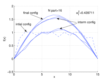
config	R(u)	$T$	N iter
initial	$0.396959$	$1\cdot 10^{-4}$	0
interm 1	$0.083343$	$1\cdot 10^{-4}$	$1\cdot 10^{3}$
interm 2	$0.048746$	$1\cdot 10^{-4}$	$2\cdot 10^{3}$
interm 3	$0.045338$	$1\cdot 10^{-4}$	$3\cdot 10^{3}$
final 16	$0.043871$	$1\cdot 10^{-6}$	$1\cdot 10^{4}$

Table 1: Rayleigh’s quotient for the configurations of figure 1 with $Npart=16$. Temperature and number of algorithm iterations are also shown.

The selection of $n=16$ or hereafter $Npart=16$ was not arbitrary. A few number of particles at the beginning of the run makes the algorithm to run faster at large values of the prescribed $F(u)$ (we can call it the “energy” of the system). As this “energy” goes down, the algorithm starts to slow down its convergence rate due to the finite number of particles. At this stage, we increment the number of particles as many times as it is necessary to get further significant reductions. This process has been named “stable resizing” due to the “resize” of the number of considered particles. Figure (2) shows the results for $Npart=64$. The exact solution (fundamental mode) appear in full line and the function that results of the minimization process is shown in cross line. The numerical values of Rayleigh quotient are presented in table (2). It can be noted that the difference between the exact and obtained $R(u)$ is below 0.01% which demonstrates the convergence of the method to the exact solution.

Figure 2: Final configuration $\times$ (cross) and exact solution $-$ (full line) for the Helmholtz equation with $Npart=64$.

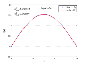
config	R(u)	$T$	N iter
final 64	$0.0438650$	$1\cdot 10^{-9}$	$5\cdot 10^{4}$
exact	$0.0438649$	–	–

Table 2: Rayleigh’s quotient for the final configuration of figure 2 with $Npart=64$. Here, the difference between the exact solution and the solution provided by the algorithm (final configuration) differs only in $0.01\%$.

VI.2 Langevin approach to the Helmholtz equation

For the case of the Helmholtz equation $u^{\prime\prime}(x)+\lambda u(x)=0$, we have already shown that the corresponding functional is $F(u)=\int_{0}^{L}(u^{\prime}(x))^{2}dx/\int_{0}^{L}u(x)^{2}dx$ which, in its discretized version is

$$F(u_{l})=\mathop{\displaystyle\sum}_{l=1}^{n}(\nabla u_{l})^{2}\delta x_{l}/\mathop{\displaystyle\sum}_{l=1}^{n}u_{l}^{2}\delta x_{l}$$ (23)

where $\nabla u_{l}=(u_{l+1}-u_{l})/\delta x_{l}$. With this form of $F(u_{l})$ and applying an Euler updating scheme Batrouni87 , it can be substituted in (19) to give

$$u_{l}(t+\delta t)=u_{l}(t)-\delta t\left(-2\frac{(u_{l+1}-2u_{l}+u_{l-1})/\delta x_{l}+\lambda u_{l}\delta x_{l}}{\|u_{l}\|^{2}}\right)$$

$$+\sqrt{\delta t}\sqrt{2D(T)}\eta_{l}(t)$$

where

$$\|u_{l}\|^{2}=\mathop{\displaystyle\sum}_{l=1}^{n}u_{l}^{2}\delta x_{l}$$

Figure 3: Initial, intermediate and final configurations for the Helmholtz equation with fixed ends for the simulations with the Langevin approach, showing the convergence of the algorithm to the minimum of the functional, $Npart=16$.

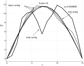
Fixed boundary conditions are also considered in this case. Numerical values of the obtained configurations are presented in table (3) where the number of algorithm iterations is also shown for time’s estimation calculations.

config	$R(u)$	$T$	N iter
initial	0.273213	–	0
interm 1	0.115614	$1\cdot 10^{-2}$	$1\cdot 10^{4}$
interm 2	0.053995	$1\cdot 10^{-3}$	$1\cdot 10^{4}$
interm 3	0.044929	$1\cdot 10^{-4}$	$1\cdot 10^{4}$
interm 4	0.044005	$1\cdot 10^{-5}$	$1\cdot 10^{4}$
interm 5	0.043875	$1\cdot 10^{-6}$	$1\cdot 10^{4}$
final 16	0.043866	$1\cdot 10^{-7}$	$1\cdot 10^{4}$

Table 3: Rayleigh’s quotient for the configurations of figure 3 with $Npart=16$ for simulations with Langevin approach. Temperature $T$ and number of algorithm iterations are also shown.

A stable resizing routine could also be applied in this case. The results for $Npart=64$ are shown in table (4).

config	$R(u)$	$T$	N iter
final 64	0.0438661	$1\cdot 10^{-8}$	$1\cdot 10^{4}$
exact	0.0438649	–	–

Table 4: Rayleigh’s quotient for the final configuration of the simulations with Langevin approach with $Npart=64$; the exact value of Rayleigh’s quotient is shown for comparison.

VI.3 Case 2

For the fourth order beam equation, $u^{(IV)}(x)-\lambda u(x)=0$, the corresponding functional is

$$F(u)=\frac{\mathop{\displaystyle\int}_{0}^{L}(u^{\prime\prime}(x))^{2}dx}{\mathop{\displaystyle\int}_{0}^{L}u(x)^{2}dx}$$ (24)

Clamped boundary conditions are considered for this case, i. e. $u(0)=u(L)=\partial u(x)/\partial x|_{x=0}=\partial u(x)/\partial x|_{x=L}=0$. As it was done before, the jump estimation can be calculated from equation (15) resulting in the same expression as (22). The only change is in $\epsilon(u)=2G(u)/||u||^{2}$. This time, $G(u)$ is

$$G(u)=\int(u^{(IV)}-\lambda u)dx$$ (25)

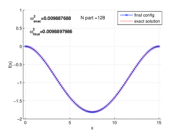
We start the algorithm with a sinusoidal function, $\mathbf{q_{0}}$, which is not the solution of the differential equation in this case (see Figure 4). This was made to illustrate that the algorithm converges to the solution of the ODE independently of the initial condition that has been employed. In figure (4) we also show the convergence of the algorithm to the solution of the beam equation as temperature $T$ goes down. The number of particles is $Npart=16$ for the first step of the process as was explained before. Numerical values are shown in table (5).

config	R(u)	$T$	N iter
initial	0.0372191	$5\cdot 10^{-6}$	0
interm 1	0.0168120	$1\cdot 10^{-6}$	$2\cdot 10^{4}$
interm 2	0.0144376	$7.5\cdot 10^{-7}$	$4\cdot 10^{4}$
interm 3	0.0123598	$2.5\cdot 10^{-4}$	$6\cdot 10^{4}$
final 16	0.0098999	$1\cdot 10^{-9}$	$2\cdot 10^{5}$

Table 5: Rayleigh quotient for the configurations shown in figure 4 (fourth order beam equation); $Npart=16$. Temperature $T$ and the number of iterations are also shown.

Figure 4: Initial, final and intermediate configurations as the algorithm runs towards the solution of the beam equation with clamped ends. $Npart=16$.

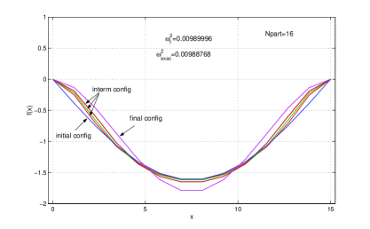
To improve the precision of the algorithm and accelerate its convergence, the number of particles were increased five times ($Npart=128$) with respect to its initial value. The final results can be observed in figure (5) where the Rayleigh quotient $R$ is also shown. It is noticeable the better accuracy of the attained solution due to the “stable resizing”.

Figure 5: Final configuration $\times$ (cross) and exact solution $-$ (full line) of a beam with clamped ends; $Npart=128$.

VI.4 Case 3

For the fourth order beam deflection under a static load the equation is $u^{(IV)}(x)=g(x)$. We have selected a concentrated load of the form $g(x)=\delta(x-x_{a})$ being $\delta(x)$, the Dirac delta function. This time, the functional is

$$F(u)=\int_{0}^{L}(u^{\prime\prime}(x))^{2}dx-2\int_{0}^{L}u(x)g(x)dx$$ (26)

Simply supported boundary conditions are selected this time, $u(0)=u(L)=\partial^{2}u(x)/\partial x^{2}|_{x=0}=\partial^{2}u(x)/\partial x^{2}|_{x=L}=0$. In this case, the functional simply represents twice the potential energy in a beam subjected to the transverse force $g(x)$. Applying equation (14) one is able to obtain the estimated jump which results

$$\delta\overline{u}=\frac{-\ln(1/2)T+2\delta u(x_{a})}{2G(u)}$$ (27)

where $G(u)=\int u^{(IV)}dx$. This equation states that the estimated jump could be obtained once $\delta u(x_{a})$ is provided. Since we have no knowledge of this quantity, it is reasonable to propose to be of order of $\delta\overline{u}$. With this assumption, equation (27) results

$$\delta\overline{u}=-\frac{\ln(1/2)T}{2(G(u)-1)}$$ (28)

The algorithm was initialized with an initial configuration of the form of a sine function with random noise. This configuration, together with intermediates and final configurations are shown in figure (6). $Npart=16$ was chosen again since it provides good initial results. Numerical values of the different configurations are shown by table (6) for $x_{a}=0.5L$, where we rename $I(u)\equiv F(u)$ .

config	$I(u)$	$T$	$Niter$
initial	1.7231	$1\cdot 10^{-4}$	0
interm 1	0.1172	$1\cdot 10^{-4}$	$1\cdot 10^{3}$
interm 2	0.001995	$1\cdot 10^{-4}$	$5\cdot 10^{3}$
interm 3	-0.0038	$1\cdot 10^{-4}$	$1\cdot 10^{4}$
interm 4	-0.00808	$1\cdot 10^{-6}$	$2\cdot 10^{4}$
interm 5	-0.01103	$1\cdot 10^{-7}$	$1\cdot 10^{5}$
final	-0.011334	$1\cdot 10^{-8}$	$2\cdot 10^{5}$

Table 6: Functional value, $I(u)$, for the case of the elastic beam equation under a static force of delta type with simply supported boundary conditions.

Figure 6: Initial, final and intermediate configurations in the convergence to the solution of a beam under static load; $Npart=16$.

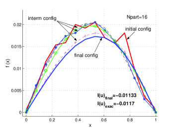
If a better precision wants to be reached, more particles must be included. Nevertheless with $Npart=16$ the difference between the exact and final solution is below 3%.

VII CONCLUSIONS

A statistical approximation to the solution of ODEs were presented, in particular we solved some problems related with vibration theory. The developed method establishes a way to attain the solution of an ODE proposed to solve physical problems, from statistical mechanics. The developed idea consists of thinking the domain of any functional (representing the ODE) as microstates of a thermal system (particle system) in contact with a heat bath at temperature $T$, that interacts trough a thermodynamic potential represented by the functional. Then, obtaining the minimum of the thermodynamic potential of this equivalent problem when $T\rightarrow 0$ is the same as to get the solution of the ODE. If only one solution exists, our method provides the unique solution of the ODE. In case we treat an eigenvalue equation, where infinite solutions exist, we obtain the absolute minimum of the corresponding functional or fundamental mode, as well as the fundamental eigenvalue.

Three examples have been provided to show the convergence of method to the solution of the ODEs; the first two of them, represents a typical eigenvalue problem, as it is the case for the Helmholtz equation and the fourth order beam equation, with infinite possible solutions. In these cases the method have shown to converge to the fundamental mode. For the third case, the beam equation under a static load, the method converge to its unique solution. Additionally, a resizing of the corresponding one dimensional lattice called “stable rezising”, which increases the discretization, was used to provide further reductions of the functional accelerating its convergence and improving its precision.

In the same spirit, a general approach to the problem within an stochastic framework was presented with similar success. We proposed an equivalent Langevin equation for the scalar field $u$ in its way to find the minimum of the functional, solution of the ODE. Numerical experiments have been run that showed that the method also converges to the exact solution for the Helmholtz equation. Of course, the other two cases, analyzed with the first developed method, can be treated within the same scheme but, for the sake of brevity, we postpone them for future works.

Summarizing, the present article does not pretend to claim a place as an alternative method to other numerical, probably faster and more precise, methods. Its virtue consists in that it is possible to establish a link between the problem of finding the solution of ODEs and an interacting particle system which can be treated by statistical mechanics; in this sense, we showed that some typical thermodynamical equilibrium variables, such as entropy and specific heat, could be in principle calculated. This provides a different perspective and new insights in solving ODEs.

VIII Acknowledgments

M. F. and S. A. V. were supported by CONICET (Argentina) and by Secretaría General de Ciencia y Tecnología of Universidad Nacional del Sur at the Department of Physics.

Appendix A

When modelling a thermal system in equilibrium, the supportive mathematical structure is simple and not exclusive of physical systems. In this mathematical structure, the entropy $S$ is defined over a convex subset $\sum$ of $\mathbf{R}^{m+1}$, where a point of $\mathbf{R}^{m+1}$ is denoted by $(X_{0},X_{1}....X_{m})$ so it can be defined a $C^{1}$ function
$S:\Sigma\rightarrow\mathbf{R}$
such that Evans02 :

• $S$ is concave

• $\frac{\partial S}{\partial E}>0$, being $E=X_{0}$

• $S$ is positively homogeneous of degree 1

For a probabilistic model there is also a measure needed, then, the requirement is fulfilled if:

• there is a class $\mathcal{A}$ defined by $\mathcal{A}=\{\rho:\;\Omega\rightarrow(0,\infty)\}$ ( in physical systems, a point of $\Omega$ is called a microstate)

• $\rho$ is $\pi-measurable$, ($\pi$ is the reference measure)

• $\int_{\Omega}\rho\;d\pi\,=1$, ( $\rho$ is the density of the microstate measure $\rho d\pi$)

• $E(X,\rho)=<\mathbf{X}>=\int_{\Omega}\mathbf{X}\rho\;d\pi$, ($X$ is called an observable).

There is a well known theorem Evans02 which ensures that

$$\sigma=\frac{\exp{(-\beta\cdot X)}}{Z}$$ (29)

maximizes $S(\rho)$ for all possible $\rho\in\mathcal{A}$. Here, $\beta\in\mathbf{R}^{m+1}$ and

$$Z=\int_{\Omega}e^{-\beta\cdot X}\,d\pi$$ (30)

References

- (1) F. Hildebrand, 1973. Methods of applied mathematics. Eudeba University Press.
- (2) W. Kaplan, 1985. Advanced Calculus. CECSA Editors.
- (3) K. Rektorys, 1975. Variational methods in mathematics, physics and engineering. D. Reidel Publishing Co.
- (4) D. Chandler, 1987. Introduction to modern statistical mechanics. Oxford University Press.
- (5) A. Sommerfeld, 1956. Thermodynamics and statistical mechanics. Academic Press.
- (6) L. C. Evans, 2002. Entropy and partial differential equations. Dept. Math. Berkeley.
- (7) L. E. Reichl, 1998. A Modern Course in Statistical Physics, 2nd Edition, Wiley.
- (8) S. Kirkpatrick, C. D. Gelatt, M. P. Vecchi, 1983. Optimization by simulated annealing. Science 220 (4598), 671-680.
- (9) G. G. Batrouni, B. Svetitsky, 1987. Accelerated dynamics in simulations of first-order phase transitions. Phys. Rev. B. 36,10 pp5647-5650.
- (10) D. E. Newland, 2006. Mechanical Vibration Analysis and Computation, Dover, Mineola, NY, USA.
- (11) A. W. Leissa, 2005. The historical basis of the Rayleigh and Ritz methods. Journal of Sound and Vibration 287 pp 961-978.
- (12) A. Metropolis, W. Rosenbluth, M. N. Rosenbluth, H. Teller, E. Teller 1953. Equation of static calculations by fast computing machines. Journal of Chemical Physics 21 (6), 1087-1092.
- (13) B. Ceranic, C. Fryer, R. W. Baines, 2001. An application of simulated annealing to the optimum design of reinforced retaining structures. Comp. and Struc. 79, pp1569-1581.
- (14) G. H. Fredrickson, V. Ganesan, F. Drolet, 2002. Field-Theoretic Computer Simulation Methods for Polymers and Complex Fluids. Macromolecules 35, pp 16-39.
- (15) N. G. Van Kampen. 1987, Stochastic Processes in Physics and Chemistry, North-Holland, Amsterdam, The Netherlands.
- (16) Numerical Recipes in C: The art of scientific computing, 1988. Cambridge University Press.