The complex galaxy cluster Abell 514:
New results obtained with the XMM - Newton satellite

Abstract

Aims. We study the X-ray morphology and dynamics of the galaxy cluster Abell 514. Also, the relation between the X-ray properties and Faraday Rotation measures of this cluster are investigated in order to study the connection of magnetic fields and the intra-cluster medium.

Methods. We use two combined XMM–Newton pointings that are split into three distinct observations.

Results. The data allow us to evaluate the overall cluster properties like temperature and metallicity with high accuracy. The cluster has a temperature of 3.8$\pm$0.2 keV and a metallicity of 0.22 $\pm$0.07 in solar units. Additionally, a temperature map and the metallicity distribution are computed, which are used to study the dynamical state of the cluster in detail. Abell 514 represents an interesting merger cluster with many substructures visible in the X-ray image and in the temperature and abundance distributions. These results are used to investigate the connection between the ICM properties and the magnetic field of the cluster by comparing results from radio measurements. The new XMM–Newton data of Abell 514 confirm the relation between the X-ray brightness and the sigma of the Rotation Measure ($S_{\rm X}$ - $\sigma_{\rm RM}$ relation) proposed by Dolag et al. (2001).

1 Introduction

It is now well accepted that the intra-cluster medium (ICM)in clusters of galaxies is magnetized. The magnetic fields can be traced by diffuse cluster wide synchrotron radio emission (Giovannini et al. 1991, 1993, Feretti 1999 and Feretti & Giovannini 2007) or Inverse Compton hard X-ray radiation caused by relativistic electrons. Additionally, an indirect measure of the strength of magnetic fields is the rotation measure (RM), in which radiation from background radio sources is studied: according to the strength of the magnetic field inside the cluster, the polarization angle of the radio emission is rotated. The different observations lead to the conclusion that magnetic fields in clusters of galaxies have strengths of a few $\mu$G (Carilli & Taylor 2002).
Dolag et al. (2001) showed that a relation exists between the X-ray surface brightness and the root mean square scatter ($\sigma_{\rm RM}$) of the Faraday Rotation Measures ($S_{\rm X}$ - $\sigma_{\rm RM}$ relation) that are used to evaluate the strength of the magnetic field. This relation is an important tool to study the connection between the magnetic field and the intra-cluster gas density and temperature (Dolag et al. 2001). In particular clusters with polarized extended radio sources are of interest, because it is possible to evaluate the RM scatter well. More sources in one cluster give the possibility to get values for the magnetic field strength in different parts of the cluster, and are therefore very important observational objects to understand the relation between the magnetic field and the X-ray properties. In order to compare the magnetic field and other cluster properties at the position of each radio source an X-ray image is required. The surface brightness $S_{\rm X}$ and the RMS can be determined at the position of each radio source.
Since Abell 514 has several radio sources that offer the possibility to study the $S_{\rm X}$ - $\sigma_{\rm RM}$ relation, it was chosen for our study. In this paper, we present results from three XMM–Newton observations of this cluster.
Throughout the paper, a $\Lambda$CDM ($\Omega_{\Lambda}$ = 0.7 and $\Omega_{\rm m}$ = 0.3) cosmology with a Hubble constant of 70 km s^-1 Mpc^-1 was assumed.

1.1 Connection of the magnetic field and the ICM density

The two observables $S_{\rm X}$ and the RMS scatter ($\sigma_{\rm RM}$) compare the two line of sight integrals:

$$S_{\rm X}\propto\int{n^{2}_{\rm e}\sqrt{T}dx}\leftrightarrow\sigma_{\rm RM}\propto\int{n_{\rm e}B_{\|}dx}$$ (1)

where n_e is the electron density and $B_{\|}$ the magnetic field component parallel to the line of sight. (Dolag et al. 2001; Clarke et al. 2001)

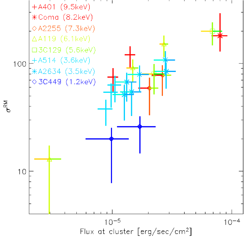
Figure 1: The scatter of the root mean square of the Faraday Rotation measure (RMS) against the X-ray flux of a sample of clusters, for which both measurements are available.

When $\sigma_{\rm RM}$ is plotted versus the X-ray flux a clear relation can be seen. This relation can be fitted by:

$$\sigma_{\rm RM}=A\Big{(}\frac{S_{\rm X}}{10^{-5}\mbox{erg}/\mbox{cm}^{2}/\mbox{s}}\Big{)}^{\alpha}$$ (2)

A simple interpretation of this relation (e.g. assuming the temperature within the ICM and the scale-length of the magnetic field to be fixed) is that the slope $\alpha$ reflects the scaling of the magnetic field strength ($B$) with the electron density ($n_{e}$). An exact relation between these two scalings, $B$-$n_{\rm e}$ and $\sigma_{\rm RM}$-$S_{\rm X}$, is derived in Dolag et al. (2001) assuming a simplified model for galaxy clusters. Note that the uncertainties in the 3D position of the individual sources (which are not known) lead to significant uncertainties in the derived $\sigma_{\rm RM}$ and therefore imprints a substantial scatter in the scaling relation. In fact this is the largest contribution to the the error bars we calculate for $\sigma_{\rm RM}$ (see Dolag et al. 2001 for details).

Additionally, it seems that there is a suspected dependence on the cluster temperature: clusters with a high overall temperature also seem to have high $\sigma_{\rm RM}$ values (see Fig. 1). To study such matter in detail, clusters that contain radio sources have to be investigated very accurately in radio and X-rays.

2 Abell 514

The cluster of galaxies Abell 514 is of Rood-Sastry type F, richness class 1, and lies between type II and III in the Bautz-Morgan classification. The cluster was first identified by George Abell 1958 using the National Geographic Society Palomar Observatory Sky Survey (Abell 1958). In 1966 it was observed by Fomalont & Rogstad (1966) during a radio survey at the 21 cm line. Waldthausen et al. (1979) mapped this cluster using the wavelength $\lambda$ = 11.1 cm. The optical centre is indicated by Abell et al. (1989) at RA(J2000) 04:47:40 and DEC(J2000) -20:25.7. Earlier X-ray observations were performed with ROSAT and Einstein and revealed a highly interesting X-ray morphology (e.g. Govoni et al. 2001).
This cluster is very special in several ways. A very prominent characteristic is the rich morphology that can be seen in ROSAT images. In contrast to a spherical, relaxed cluster Abell 514 seems to be in a phase of ongoing merging, making it an example for the study of dynamical events connected with cluster formation. Another important point is the fact that six extended radio sources lie inside the cluster. These radio sources were studied in detail by Govoni et al. (2001), who derived information on the strength and structure of the cluster magnetic field by starting from Faraday Rotation measurements. Three of these sources are within the central field of view of the XMM–Newton observations which we present in this paper.
Govoni et al. (2001) found observational evidence for the existence of a strong magnetic field. The strength of the magnetic field was estimated to be 4-7 $\mu$G in the centre with a coherence length of 9 kpc. They also give the $\sigma_{RM}$ of the radio sources that can be seen in the cluster region. Three of them - B2, D North and D South - (Marked as B2, D north and D south in Fig. 2) are inside the field of view of the XMM observations and will be presented in this paper. The radio source B1 was found only marginally polarized by Govoni et al. (2001) and is not used as a data point for the $S_{\rm X}$ - $\sigma_{\rm RM}$ relation.

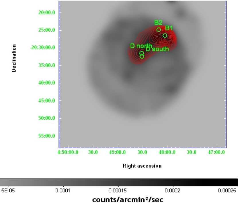
Figure 2: The location of three of the radio sources within the cluster Abell 514 (D_north and D_south are measurements from the same source, but in two slightly offset positions). The other three radio sources lie outside the field of view of this X-ray observation.

3 Observations and data reduction

The data we analyse in this paper result from two different XMM–Newton pointings, split into three distinct observations. The first observation took place in 2003, February 7th, the second in 2003, March 16th. In 2005, August 15th the cluster was observed for a third time. All observations were performed with the European Photon Imaging Camera (EPIC) using the medium filter in full frame mode. Table 1 displays the exposure times for the individual observations.
For the third observation, CCD number six from the MOS 1 camera was switched off, because of an incident that occurred during revolution number 961 (the camera was hit by a micrometeroid). Therefore, this camera is only used for our analysis when the studied area does not lie inside the affected region.

Table 1: Total and effective exposure times

Camera	Obs. 1 (s)	Obs. 2 (s)	Obs. 3 (s)
MOS1 tot.	14963	14959	15571
MOS1 eff.	9388	5269	5026
MOS2 tot.	14963	14954	15580
MOS2 eff.	9355	5585	5486
PN tot.	13388	13337	14148
PN eff.	5007	3506	3922

The data were reduced using SAS version 6.5.

All three observations are heavily polluted by solar flares. The times with high count rates are therefore rejected. The rejection of times with high count rate is done by creating good time interval tables with defining an upper threshold for the count rates for each camera and observation. The times with count rates above the threshold are rejected and new data sets containing only the flare-free times produced. This threshold was defined using the count rates in the high energy (10 - 12 keV for MOS1 and MOS2, 12 - 14 for PN camera) bands. Times where the count rate was high and also changing with time, were cut out. We also had a look how the exposure time changes with the threshold: this curve has at first a steep slope if we take very low thresholds (cutting away most of the observation time) and gets shallow with high threshold (cutting away no observation time). A good criterium to choose the threshold is to take the point where the slope starts to change. The original and resulting exposure times are listed in Table 1.
To study the diffuse emission of the ICM, point sources are also removed. This is done by a combination of a source list provided from the Science Operations Centre (SOC) of XMM data processing and visual inspection. For each camera and observation, region files that are to be excluded for the further analysis are created. We also check if point sources are coincident with the radio sources. However, this is only the case for B2. For the flux calculation, the reduced area is taken into account.
Also, the images are corrected for the vignetting effect. To achieve this, we use two different methods. For the image preparation - especially to get exposure corrected mosaic images - we produce an exposure map and divide the images by this. Additionally, the method proposed by Arnaud et al. (2001) is used to correct for vignetting. Here, every photon is multiplied by a weight factor according to its position on the detector.
Since the PN camera images have many bright columns, they are not used for the production of a mosaiced and smoothed image. However, for the spectral analysis, we use the data from those cameras as well. The areas that show bright pixels or columns are removed by using a mask.
Another important reduction step is the correct background subtraction. The XMM background consists of three parts (a cosmic X-ray background (CXB), the background produced by soft proton flares and a non X-ray cosmic background (NXB) induced by high energy protons). The soft proton flares are already removed from the data files in the first reduction step, when the flare free event files are produced. To get rid of the CXB and the NXB we use the double-subtraction method proposed by Arnaud et al. (2002) throughout the spectral analysis.

4 Results

4.1 Morphological Analysis

To study the structure of the cluster in detail, we produce a mosaic image of the MOS cameras of all three observations using the energy band between 0.3 and 10 keV (see fig. 3). This image is smoothed using an adaptive smoothstyle and a signal to noise ratio (SNR) of 40 (see fig. 5). The adaptive smoothstye is especially created for poissonian images like X-ray images. Here, every pixel is assigned with a desired SNR and is then smoothed towards this SNR by a weighted cyclic convolution. We tried smoothing the image with different SNR and settled for a SNR of 40, because with this value the structure of the image is kept and the borders are not smoothed or enhanced in brightness too much.

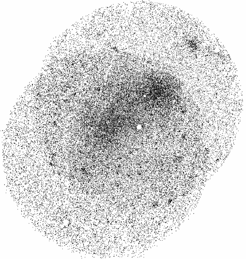
Figure 3: A mosaic image of the MOS cameras of the three different observations. The image is exposure corrected. The field of view of the observation is about 37$\times$28 arcmin.

The size of the whole field of view of the observation has a length of 37 and a width of 28 arcmin. This corresponds to a size of 3.0 Mpc x 2.3 Mpc. The ICM emission seems to be elongated along a filament/main axis over the length of 1.6 Mpc. In the direction perpendicular to this axis, the cluster emission can be detected out to 0.8 Mpc.

The X-ray centre lies at RA 04:48:04 (J2000) and DEC -20:26:42 (J2000). The area with the brightest X-ray emission is not a clear point-like feature. This might be the main reason that this value differs from the result of earlier observations (Govoni et al. 2001), which give the X-ray centre at RA 04:48:13 (J2000) and DEC -20:27:18 (J2000). It also depends on the used smoothing method. The most important point to mention here is however the differently sized point spread function (PSF) of ROSAT and XMM–Newton: ROSAT’s PSF is considerably larger (about 1 arcmin vs. 5-6 arcsec). This together with the different smoothing methods applied can explain the offset between the two positions for the X-ray centre. Especially with a cluster as inhomogeneous as Abell 514 the exact positioning of a centre is very dependant on smoothing techniques and detector sensibility.
In Fig. 4 we show the X-ray contours superposed on an optical image of the cluster (image taken from Aladin Previewer, Space Telescope Science Institute). The two subclumps that can be seen in the X-ray image correspond to the galaxy distribution of the optical image. The X-ray centre is offset with respect to the optical centre, which is at RA 04:47:40 (J2000) and DEC -20:25.70 (J2000) (Abell et al. 1989). This offset can be explained by the fact that Abell 514 is a merger cluster. If we assume that the Northwest peak has undergone a merger in recent times (more evidence for this scenario is also discussed in section 4.2 and 5.) the fact that the galaxy and gas distributions are offset is not surprising.

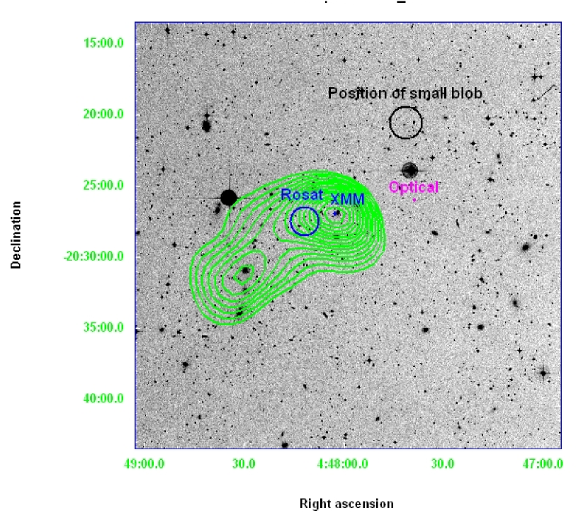
Figure 4: The optical image overlayed with the X-ray contours. The two main X-ray clumps correspond well with the distribution of the galaxies, especially the area around the most X-ray bright emission shows the highest density in galaxies.

The rich substructure that hints at a merger cluster can be seen clearly in Fig. 5. To the Northwest of the main cluster a small blob-like feature is also visible. In the optical image there are galaxies with cluster redshift seen in the area of this blob. Therefore we conclude that this is most likely another subpart of the cluster, which is infalling along the main axis and will merge with the cluster. It is about 500 kpc away from the closest part of the rest of the cluster and no connection can be seen towards the cluster. The brightest peak of the main cluster shows a steeper decline in surface brightness in the outwards direction than in the direction towards the second X-ray peak. This feature will be addressed later (see Sect. 5.1).

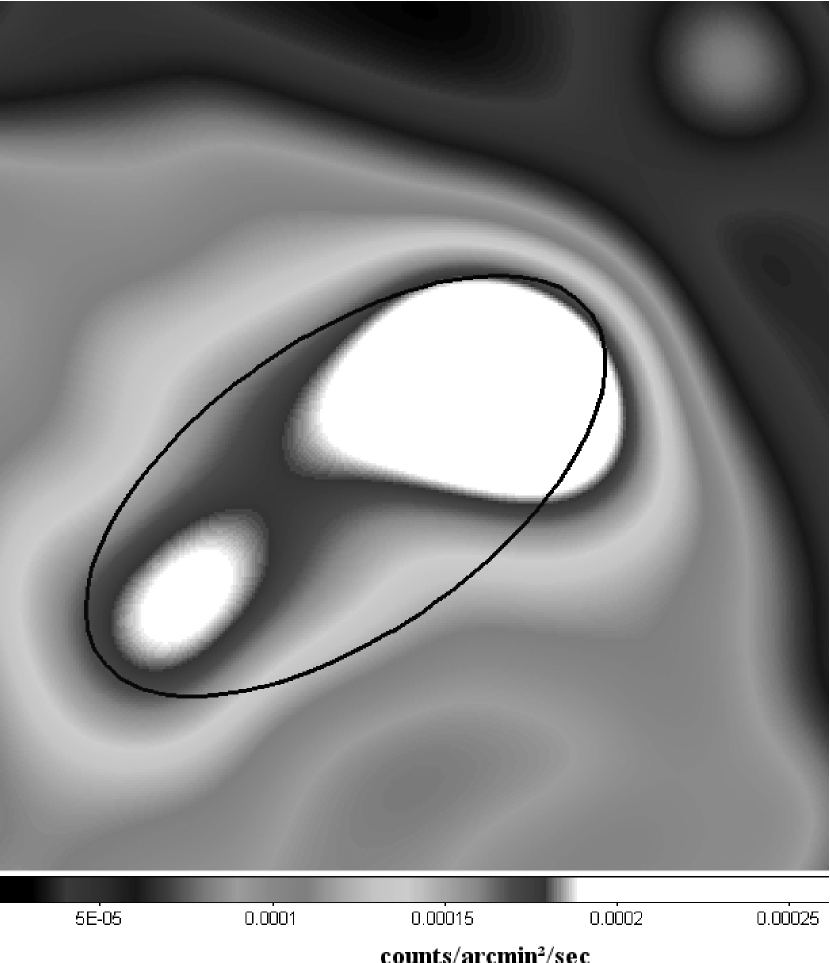
Figure 5: A smoothed image of the whole cluster. This image is corrected for vignetting and smoothed with an adaptive smoothstyle with a signal to noise ratio of 40. It shows two subclumps and the overall elongated shape of the cluster. The size of the box is about 25 arcmin ($\sim$ 2.05 Mpc). The elliptical region indicates the area where we extracted a spectrum for the whole cluster.

Around both main peaks visible in the image, the X-ray brightest one to the Northwest (NW) and the second brightest one to the Southeast (SE) of the cluster, we extract a surface brightness profile (see Fig. 6). In both cases we chose regions that seem to be mostly unaffected by the merger between those two subparts. To do this, we selected the areas where no obvious substructures can be seen in the image (see Fig.6). In particular, we adopted wide-angular regions pointing outwards from the area connecting the two peaks, where instead substructures can be seen both in the image and in the temperature map (see Fig.9). To correct for vignetting, a weight factor is applied to the data. The background is again subtracted using the double background subtraction method.
The profile for the NW peak is shown in Fig. 7. Apart from one bump around $\sim$1.5 arcmin from the centre, the profile around the NW peak does not show any irregularities like bumps or similar structures. It is noticeable, that the decline between roughly 1.0 and 2.5 arcmin from the centre is steep compared with a relaxed cluster. For a relaxed cluster, the surface brightness profile can be fitted very well with a single $\beta$ profile:

$$S_{\rm X}(r)=S_{\rm X,0}\Big{[}1+\Big{(}\frac{r}{r_{\rm c}}\Big{)}^{2}\Big{]}^{(0.5-3\beta)}$$ (3)

Here, $S_{0}$ is the central surface brightness, $r_{\rm c}$ the core radius and $\beta$ the slope parameter. In the case of a relaxed cluster, $\beta$ has a value of roughly 0.6. If we try to fit the profile of Abell 514 with a single $\beta$ profile, we get a value of 1.98 for $\beta$. This again shows that it is not a relaxed cluster part, although no substructure is seen. The steep decline will be discussed later.

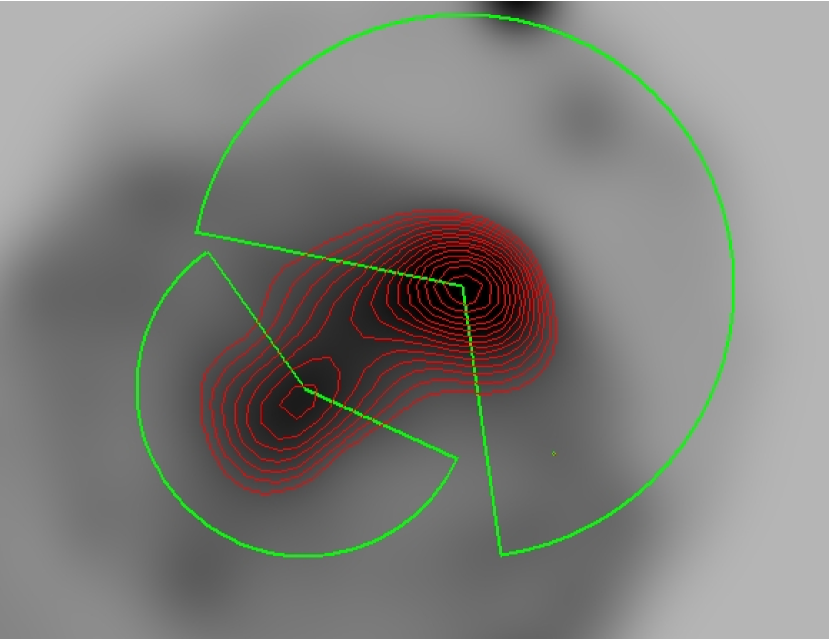
Figure 6: The image shows the regions considered for deriving the surface brightness profiles around the NW and SE peaks. Each area was divided in different annuli and the gaps in the detector and point sources were masked before extracting the surface brightness profiles.

We attempted a similar analysis around the SE peak. We choose five annuli around the center (see Fig. 6) in a direction away from the connection towards the other peak. However, this analysis was complicated by the low count rates in this region. We got indications that the surface brightness profile around the SE peak is shallower than the NW one.

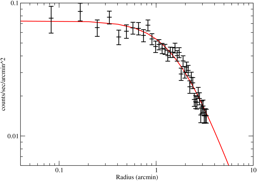
Figure 7: The surface brightness profile around the NW peak (the X-ray brightest). The profile declines rapidly outside $\sim$ 2 arcmin, a feature most likely caused by a shock due to a merger (see Sect. 5.1).

4.2 Spectral Analysis

As a first step we obtain the temperature and metallicity for the whole cluster. To get this information, we extract a spectrum in the elliptical region shown in Fig.5. This is done separately for each camera and observation to maximize the signal to noise ratio. The background is subtracted using the double subtraction method proposed by Arnaud et al. (2002). The spectra are then loaded into Xspec and fitted with a redshifted MeKaL model. To include the Galactic absorption, the Tuebinger Absorption model (tbabs) was used.
The energy range for the spectra was between 0.5 and 8.0 keV. This energy range was chosen because the distinct cameras have the best agreement in the results in this range. The redistribution matrix files (RMF) we use are calculated for the MOS cameras using the SAS task ”rmfgen”. For the PN camera we adopted the canned matrix epn_ff20_sY9_v6.8.rmf.

The cluster temperature is 3.8 $\pm$ 0.2 keV, which is consistent with the value of $\sim$ 3.6 keV estimated from the L-T relation (Govoni et al. 2001). The overall cluster metallicity is 0.22 $\pm$ 0.07 in solar units.
To study the temperature and metallicity distribution in detail, we divide the cluster into four regions and extract a spectrum in each one. This is done for all three observations for all cameras. Again, the resulting spectra are fitted in Xspec with a MeKaL model. Fig. 8 shows the regions where the spectra were extracted. The regions are chosen to contain a comparable photon signal and also give comparable statistics. The region numbers are defined in the following way: region 1 = outer region, region 2 = box around NW peak, region 3 = area between the two peaks, region 4 = box around SE peak. The final values for temperature and abundance do not change if those areas are moved around, as long as they cover the area around the NW peak, the region between the two peaks, the SE peak and the outskirts of the cluster. With the regions we give here, we are able to collect most photons per area and get better statistics then e.g. choosing circles as regions.

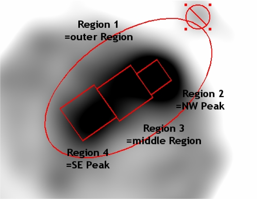
Figure 8: The four regions where temperature and abundance were estimated. The numbers correspond to the region numbers given in the temperature and metallicity diagrams.

By comparing the temperature and metallicity distribution we are able to study the dynamical state of the cluster. In Fig. 9 the temperature map which is calculated using spectra in different regions of the cluster is shown. Three regions with different temperature along the axis of the cluster can be seen, as well as a cooler outer region.

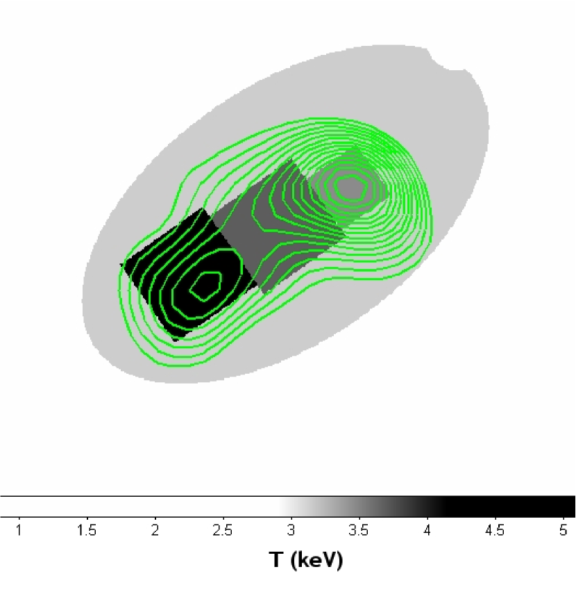
Figure 9: The temperature map of the cluster. Overlayed are the contours of the X-ray surface map. The circle represents the region where a subpart of the cluster is visible in the raw and smoothed images (see Figs. 3 and 5). This area was excluded from the spectral analysis.

The hottest region is the box number four which is located around the SE peak. It is also the one with the highest metallicity, as can be seen in the second diagram in Fig. 10. The right panel in Fig. 10 shows the metallicity distribution in the cluster. We see that the SE peak has a higher metallicity than the rest of the cluster.
Inside the error bars the temperatures derived for the NW region and the middle region can be seen as having the same temperature as the outside region. There is a trend in the cluster to have higher temperatures in the SE. The region around the SE peak is clearly the hottest of the whole cluster.

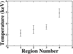
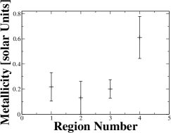
Figure 10: The temperature and the metallicity distribution in the cluster. The region numbers are as defined in Fig. 8.

The difference in metallicity between regions two and three compared to region four, can be seen as a sign that those parts of the clusters have not yet had the possibility to merge and are still infalling towards a common centre. As has been shown by Kapferer et al. (2006), a cluster has steeper gradients in metallicity before the merger process. When the subclusters have finally merged, their metallicity is smoothly distributed.

Another way to study the temperature distribution is via hardness-ratio maps. Such a map is also produced for this cluster from four different energy bands (0.3-1, 1-2, 2-4.5, 4.5-8 keV). Only the MOS1 camera of the first observation could be used for this due to technical reasons. Therefore, the count rates are very low compared to the other method and only relative differences in temperature but no absolute values can be shown. The temperature map is presented to show that the temperature distribution is very inhomogeneous. This hints at a merger cluster which is not yet relaxed but in the first stages of merging (Fig. 11).

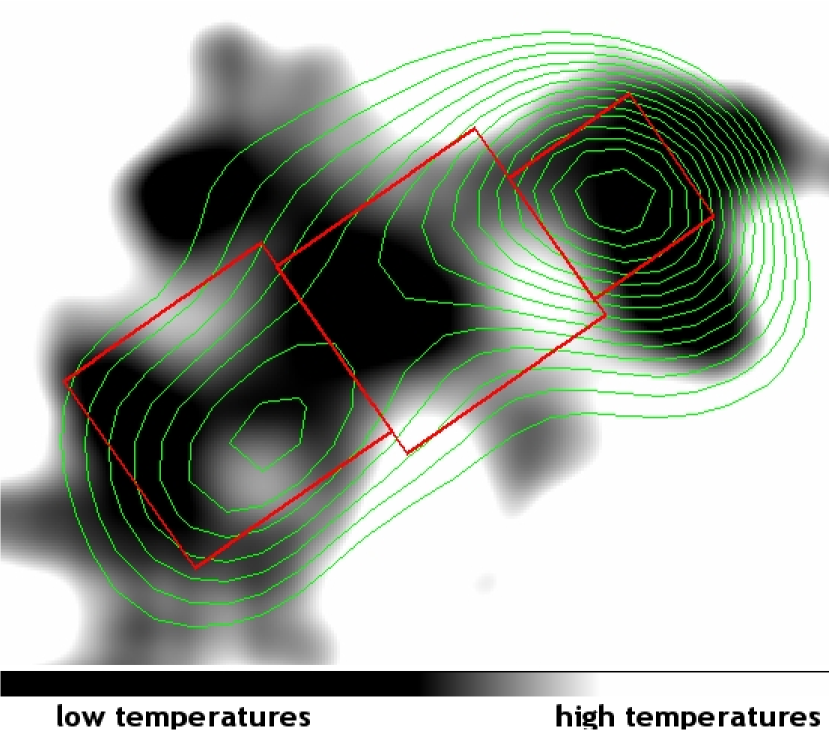
Figure 11: The temperature map created using the hardness ratio of images in four different energy bands. See text for details.

The region of the brightest X-ray peak is cool, which is in good agreement with the spectral result that also gives a low temperature for this part of the cluster. The second brightest X-ray peak has a higher temperature, again corresponding to the spectral result that gives a higher temperature for the area around this peak. The region between the two peaks seems to be a mix of high and low temperatures, corresponding to the mean temperature of the spectral result. The seperate areas with different temperatures between the two X-ray clumps cannot be seen using the spectral method, since we do not have enough photons to produce a spectrum that can be fitted reliable. We therefore see the mixing of the different temperatures. The regions in the outer parts of the cluster have too low count rates to give reliable results.

4.3 Mass determination

When we assume hydrostatic equilibrium and spherical symmetry, it is possible to calculate the mass of a galaxy cluster using the temperature and the density profiles. Although Abell 514 is a very active merger cluster and neither in a hydrostatic equilibrium nor has a spherical shape, we try to use these assumptions to calculate the mass of two subparts of the cluster. These two parts are the regions around the two X-ray brightest peaks. They show a separated emission and can be approximated as spherical symmetric in a first, rough step.
The total mass is given by the equation:

$$M_{\rm tot}(r)=-\frac{kT}{G\mu m_{\rm p}}r\Big{[}\frac{d\ln n_{\rm e}}{d\ln r}+\frac{d\ln T}{d\ln r}\Big{]}$$ (4)

where $k$ is the Boltzmann constant, $T$ the gas temperature, $G$ the gravitational constant, $\mu$ the mean molecular weight of the gas ($\mu$ $\approx$0.6), $m_{\rm p}$ the proton mass and $n_{\rm e}$ the electron density.
If the ICM follows a $\beta$-model, the electron density can be written as:

$$n_{\rm e}(r)=n_{\rm e0}\Big{[}1+\Big{(}\frac{r}{r_{\rm c}}\Big{)}^{2}\Big{]}^{-\frac{3}{2}\beta}$$ (5)

The values for $\beta$ and $r_{\rm c}$ are the values obtained by fitting a $\beta$ profile to the surface brightness of the cluster.
Inserting equation 5 into equation 4, yields:

$$M_{\rm tot}(r)=-\frac{kr^{2}}{G\mu m_{\rm p}}\Big{[}\frac{dT}{dr}-3\beta T\frac{r}{r^{2}+r_{\rm c}^{2}}\Big{]}$$ (6)

Assuming that the cluster is isothermal inside a certain radius, $\frac{dT}{dr}$ is zero. The final equation to calculate the mass inside a certain radius is therefore:

$$M_{tot}(r)=\frac{3k\beta}{G\mu m_{p}}T\frac{r^{3}}{r^{2}+r_{c}^{2}}$$ (7)

With the values we obtain by trying to fit a single $\beta$ model to the surface brightness profiles of the two brightest peaks, we are able to give at least a very rough first estimate of the masses. Since we can extract the profile of the second brightest peak only out to 5.7 arcmin ($\sim$ 490 kpc), we use this radius to calculate the mass for both regions. Using equation 7 and the results from the spectral analysis for the temperature in the different parts of the cluster (region 2 and 4, see below) the mass of the X-ray brightest part inside a radius of $\sim$490 kpc is about 3.0 10¹⁴ M_⊙, while the second clump has a mass of about 6.5 10¹³ M_⊙. This can only be seen as a crude first guess of the masses. The X-ray brightest part also seems to be the most massive one. This result can be expected from the L_X - Mass relation.

5 Discussion

5.1 Candidate for a cold front or a shock?

A prominent morphological structure of Abell 514 is a steep decline in X-ray surface brightness towards the Northwest region. This can be seen as a sharp edge in the image (see Fig. 5), as well as a quick drop of the surface brightness profile outside $\sim$ 2 arcmin (see Fig. 7).

Possible explanations for such a feature can be either a cold front or a shock caused by the merger process. Similar features were found by Markevitch et al. (2000) and Vikhlinin et al. (2002) in the clusters Abell 2142 and Abell 3667. Another example for a similar structure was also found in Abell 2256 by Sun et al. (2002). During a cluster merger, a cool core of a subpart of a cluster can survive the merging process. This is characterised by the fact that the temperature inside a brightness edge is lower than in the surrounding region. The other explanation for a feature like the one seen in Abell 514 would be a shock where the material is compressed.
To test if the edge in Abell 514 is caused by a cold front or a shock we study two regions, one inside and one outside the edge visible in the smoothed X-ray image (Fig. 5), with respect of their density and temperature. The regions used for this analysis are shown in Fig. 12.

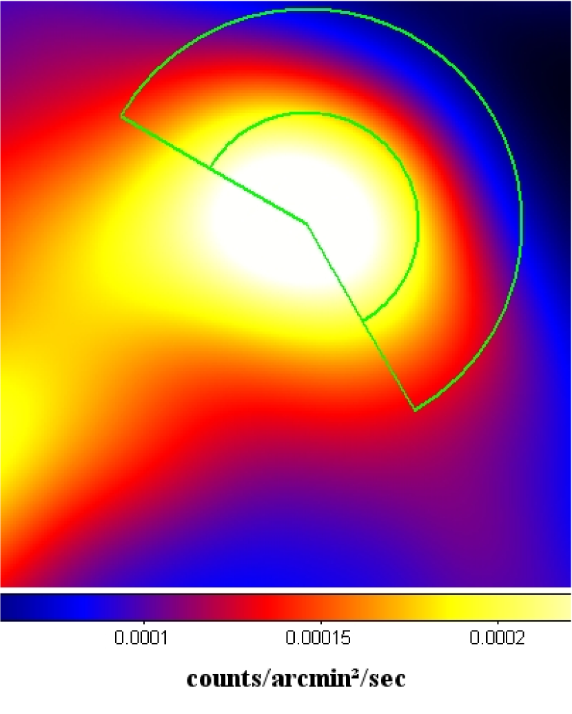
Figure 12: Regions considered for the deprojection analysis in order to investigate the nature of the drop in surface brightness.

Region 1 is the region inside the ”edge”, while region 2 is the area in the outer part. We apply the deprojection method by using the Xspec model projct to calculate densities inside and outside of this border. Also the temperatures in both regions were calculated and compared with each other. The results are shown in Table 2.

Table 2: The density and temperature inside (Region 1) and outside (Region 2) the brightness edge.

	Region 1	Region 2
Density [10-3cm-3]	0.91 $\pm$ 0.11	0.51 $\pm$ 0.06
Temperature [keV]	4.5 $\pm$ 0.8	3.6 $\pm$ 0.5

The temperature inside the border is slightly higher than outside, but no jump in temperature can be deduced from our data, especially not a jump from a cool core to a warmer surrounding. Inside the errorbars, both temperatures can be seen as the same. Therefore the discontinuity in surface brightness cannot be caused by a cold front. The density however shows a clear discontinuity. It is therefore possible that the brightness jump is due to a shock. Such a shock can be the result from an earlier merger, with the different structures not distinguishable by eye any more.
The visible interaction between the SE peak and the NW one is most likely not responsible for this feature. We see that the metallicities between the two peaks are very different. It is therefore plausible that they have not merged yet and cannot cause the feature in the surface brightness seen in the NW peak.
Another possibility could be an interaction of the main X-ray peak with the small blob from the south east part. But since this structure is still 500 kpc away from the main cluster and no connection between the two parts can be seen we do not expect to see any interaction effects yet between those parts.

5.2 The $S_{\rm X}$ - $\sigma_{\rm RM}$ relation and the magnetic field

According to theory (Tribble 1993, Dolag et al. 1999), the magnetic field is amplified in a hot merger cluster. The $S_{\rm X}$ - $\sigma_{\rm RM}$ relation is clearly dependent on the temperature of the cluster (see Sect. 1.1). For Abell 514, this general trend can be studied. Although Abell 514 is a merger cluster, its magnetic field is still quite low. This can be seen in good agreement with the low overall temperature of the cluster. Still, compared to other cool clusters, Abell 514 shows a slightly higher $\sigma_{RM}$ which is most likely due to the ongoing merger that already enhanced the magnetic field.
One main aim of the XMM–Newton observations was to get new values for the X-ray flux in the regions where the radio sources are. It has to be mentioned that the true location of these radio sources inside the cluster is not known. This fact is taken into account in the errors given for the $\sigma_{\rm RM}$ value. The error bars cover the range of values between a source located in the cluster center and one behind the cluster.

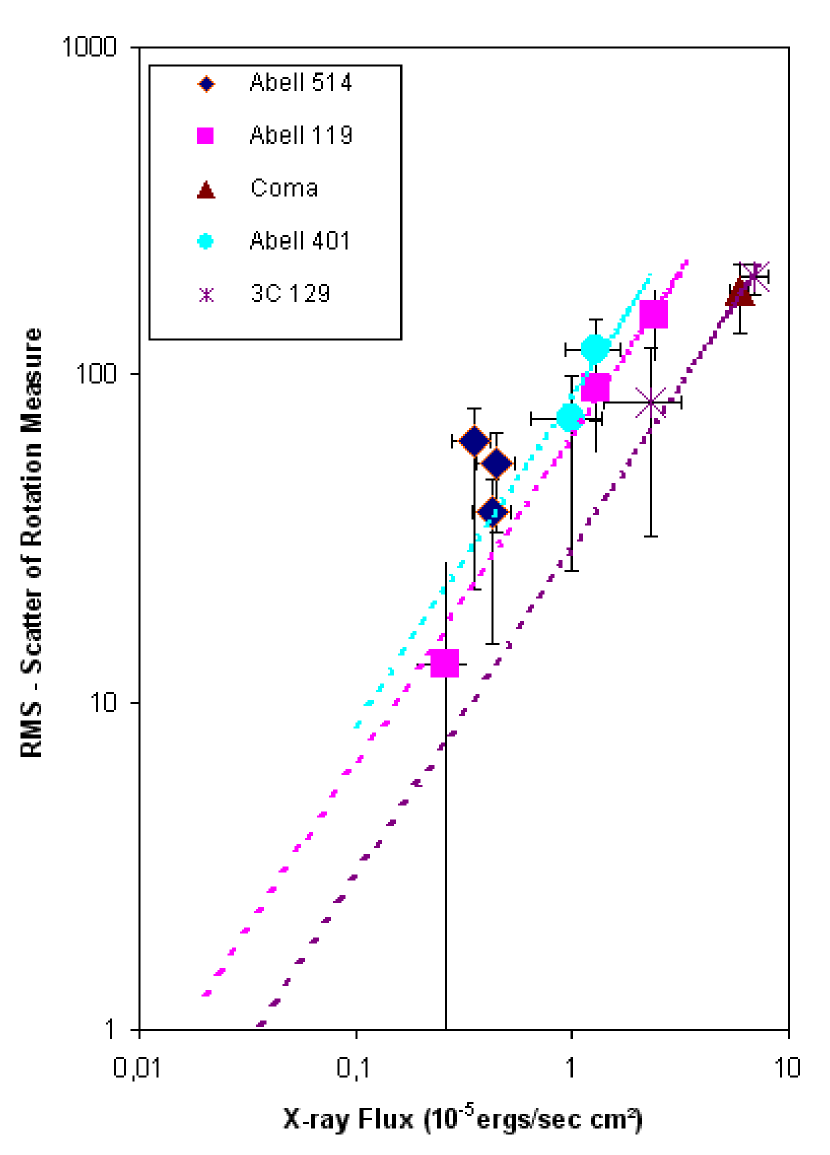
Figure 13: The X-ray flux - $\sigma_{\rm RM}$ relation with the new data points for Abell 514. The new values are in good agreement with the general slope of the relation

.

The new values are then compared to the results from measurements of the magnetic field (via the $S_{\rm X}$ - $\sigma_{\rm RM}$). They fit well with other measurements from Coma, A119 etc. (see Fig. 13). Fig. 13 shows the results from the new measurements, with the data point for the other clusters (Coma, A119, etc.) being converted to the same energy band. In general, the data points obtained for A514 are in good agreement with the relation found from the rest of the clusters. The lines in fig. 13 represent the correlations for the distinct clusters. We see that the data points of Abell 514 lie above the correlations of all the other clusters. This can be seen as an indication for an amplification of the magnetic field due to the ongoing merger in Abell 514. Overall, the points from Abell 514 make the whole correlation (if we use the observational data) less steep. Without the data points from Abell 514, the slope parameter is 1.19, while it is 0.98 with them. Inside an error of 10% both values agree. To avoid any instrumental bias in this study in the future, we plan to obtain XMM–Newton data for the other clusters in this sample as well.

Additionally, with the creation of a temperature map, it is possible to compare the strength of the RMS scatter $\sigma_{\rm RM}$ from the rotation measures with the temperature of the ICM in the area of the radio source. Table 3 shows the results.

Table 3: Comparison of $\sigma_{\rm RM}$ with the temperature. The regions are as indicated in Fig. 8

Region Nr.	T (keV)	$\sigma_{RM}(rad/m^{2})$
Region 2 (includes Radio source B2)	3.2 $\pm$ 0.2	63 ${}^{+16}_{-41}$
Region 4 (includes Radio sources Dnorth and Dsouth)	4.9 $\pm$ 0.4	54 ${}^{+12}_{-21}$ (north) 38 ${}^{+10}_{-23}$(south)

Here, $\sigma_{\rm RM}$ is lower in the hottest region and higher in the cool, X-ray brightest part, that seems to be the most relaxed part of the cluster. However, this is not in contradiction with the above relation. Inside the cluster, more complicated effects take place additionally to the overall properties, that cannot yet be resolved with the current observations. Also, the RMS measurements are taken from a smaller area than the spectra we use to deduce the temperature. Small scale fluctuations inside these regions are therefore possible and not taken into account in table 3.

6 Summary

We performed a detailed study of the X-ray emission of the merger cluster Abell 514. Three pointings by the XMM–Newton telescope were analysed to study the properties of this cluster, especially the dynamical state and the relation between the X-ray flux and the RMS of the rotation measure produced by the magnetic field inside the cluster.
The image of Abell 514 shows the rich substructure of the cluster, a clear sign for an ongoing merger. Two main X-ray bright peaks can be seen with a connection between them. The brightest peak also shows signs for a shock, most likely caused by a recent merger.
We found the overall cluster temperature to be 3.8 $\pm$ 0.2 keV. This value is in good agreement with the one from the L-T relation (3.6 keV). The cluster metallicity is 0.22 $\pm$ 0.07 solar units.
Additionally to the calculation of overall values for the temperature and the metallicity we are able to produce rough temperature and metallicity maps. To achieve this, we divide the cluster in four different regions and extracted spectra therein. With the help of these maps, we can study the dynamical state of the cluster in more detail.

It appears that the two main visible subclumps have not had time to merge yet. Their temperatures and metallicities have significantly different values. The brightest part in the Northeast shows a steep decline that could be caused by a shock due to an earlier merger. We divide this area into two regions to calculate the density and temperature inside and outside the visible edge. The obtained values indicate that the brightness edge is indeed caused by a shock.
The X-ray flux is determined in the regions where extended radio sources are. These radio sources enable the measurement of the scatter of the Faraday Rotation measures which is due to the strength of the magnetic field. They are related with the X-ray flux. With the XMM–Newton observations we are able to add new points to this $S_{\rm X}$ - $\sigma_{\rm RM}$ relation. The new data points fit well in the model predicted by Dolag et al. (2001).
The low overall temperature also confirms the relation between the ICM temperature and the magnetic field strength (lower temperature clusters have generally smaller magnetic fields). This can also be seen as a sign that the cluster is still in an early stage of the merger and has not been heated up yet, nor has the magnetic field been enhanced by the merger.

References

- Abell (1958) Abell, G. O. 1958, ApJS, 3, 211
- Abell et al. (1989) Abell, G. O., Corwin, H. G., Jr., & Olowin, R. P. 1989, ApJS, 70, 1
- Arnaud et al. (2001) Arnaud, M., Neumann, D. M., Aghanim, N., Gastaud, R., Majerowicz, S., & Hughes, J. P. 2001, A&A, 365, L80
- Carilli & Taylor (2002) Carilli, C. L., & Taylor, G. B. 2002, ARA&A, 40, 319
- Clarke et al. (2001) Clarke, T. E., Kronberg, P. P., & Böhringer, H. 2001, ApJ, 547, L111
- Dolag et al. (1999) Dolag, K., Bartelmann, M., & Lesch, H. 1999, A&A, 348, 351
- Dolag et al. (2001) Dolag, K., Schindler, S., Govoni, F., & Feretti, L. 2001, A&A, 378, 777
- Feretti et al. (1999) Feretti, L., Dallacasa, D., Govoni, F., Giovannini, G., Taylor, G. B., & Klein, U. 1999, A&A, 344, 472
- Fomalont & Rogstad (1966) Fomalont, E. B., & Rogstad, D. H. 1966, ApJ, 146, 528
- Giovannini et al. (1991) Giovannini, G., Feretti, L., & Stanghellini, C. 1991, A&A, 252, 528
- Giovannini et al. (1993) Giovannini, G., Feretti, L., Venturi, T., Kim, K.-T., & Kronberg, P. P. 1993, ApJ, 406, 399
- Govoni et al. (2001) Govoni, F., Taylor, G. B., Dallacasa, D., Feretti, L., & Giovannini, G. 2001, A&A, 379, 807
- Feretti & Giovannini (2007) Feretti, L., & Giovannini, G. 2007, ArXiv Astrophysics e-prints, arXiv:astro-ph/0703494
- Kapferer et al. (2006) Kapferer, W., Ferrari, C., Domainko, W., et al. 2006, A&A, 447, 827
- Markevitch et al. (2000) Markevitch, M., Gonzalez, A. H., David, L., Vikhlinin, A., et al. 2000, ApJ, 541, 542
- Sun et al. (2002) Sun, M., Murray, S. S., Markevitch, M., & Vikhlinin, A. 2002, ApJ, 565, 867
- Tribble (1993) Tribble, P. C. 1993, MNRAS, 263, 31
- Vikhlinin & Markevitch (2002) Vikhlinin,s A. A., & Markevitch, M. L. 2002, Astronomy Letters, 28, 495
- Waldthausen et al. (1979) Waldthausen, H., Haslam, C. G. T., Wielebinski, R., & Kronberg, P. P. 1979, A&AS, 36, 237