Pure spin current generation in a Rashba-Dresselhaus quantum channel

Abstract

We demonstrate a spin pump to generate pure spin current of tunable intensity and polarization in the absence of charge current. The pumping functionality is achieved by means of an ac gate voltage that modulates the Rashba constant dynamically in a local region of a quantum channel with both static Rashba and Dresselhaus spin-orbit interactions. Spin-resolved Floquet scattering matrix is calculated to analyze the whole scattering process. Pumped spin current can be divided into spin-preserved transmission and spin-flip reflection parts. These two terms have opposite polarization of spin current and are competing with each other. Our proposed spin-based device can be utilized for non-magnetic control of spin flow by tuning the ac gate voltage and the driving frequency.

I Introduction

Manipulation of electron spins can be achieved via applying external active control, which is the essential requirement of spintronics devices.spinintro Especially, spin-resolved current generation is one of the key interests in spintronics research for its potential application in quantum information science.Zuti:0323 ; Burk:2007 Various approaches were proposed to overcome the fundamental challenge in the issues of spin current manipulation, detection, and injection efficiency. Methods based on controlling magnetic fieldWats:8301 ; Sun:8301 ; Zhan:6602 and material ferromagnetismBrat:5304 are investigated. However, for practical applications, more efficient methods that do not involve strong magnetic field or interfaces between ferromagnets and semiconductors are still needed. Spin pumping can be a viable solution to the spin current generation.Shar:0531 ; Li:5312

Pumping of charge current is a fully quantum mechanical phenomenon in a mesoscopic system that can generate current without applied bias between two leads. Theoretically and experimentally, charge current pump has been realized and implemented in a quantum channel or a cavity in the way of periodic modulation.Thou:6083 ; Brou:0135 ; Swit:1905 ; Tang:353 ; Wang:3306 In the adiabatic regime, Brouwer proposed a clear picture that the pumped current depends on the enclosed area in parametric space which is formed by a set of periodically varied parameters. Such formalism was readily extended to non-adiabatic regime, which is valid in the whole spectrum of frequency.Vavi:5313 If the spin degree of freedom is incorporated, spin-dependent transmission coefficients can be differentiated either directly by external magnetic fieldMucc:6802 ; Benj:5318 or by spin-orbit interaction.Gove:5324 ; Li:5312 Spin pumping is generalized from the quantum pumping and exempted from the spin injection problem which occurs in the integrated semiconductor-ferromagnet architecture.

In order to achieve spin pumping, a Rashba-type narrow channel (which ignores the presence of the Dresselhaus term) driven by local time-dependent potential was proposed.Wang:5304 ; Tang:5804 When electrons propagate through the potential region, quasi-bound state feature was shown to enhance the spin-resolved transmission difference so that sizable pure spin current can be generated. However, since the Dresselhaus spin-orbit interaction is an intrinsic effect in semiconductor materials with bulk inversion asymmetry,Dresselhaus55 it is essential to take into account this effort when considering such a spin pumping device. It should be noted that the presence of the Dresselhaus term will lead to the spin-flip mechanism which can modify the spin-pumping characteristics in a qualitative way. We shall elucidate the possibility to manipulate not only the intensity but also the polarization of the spin current.

In this paper, the spin-resolved Floquet scattering matrix formalism is applied to our system.Zhan:5347 ; Wu:5412 Based on the Floquet theorem, this formalism provides an exact and nonperturbative solution to the time-periodic Schrödinger equation in the mesoscopic system. Because the time-dependent spin-orbit interaction couples two spin polarizations and all sidebands together, analytic expression for the sideband dispersion is not feasible. Thus, we determine the sideband dispersion relation numerically by solving the Schrödinger equation in a nearly complete basis. Besides, the spatial inhomogeneity can also be handled by matching boundary conditions piece by piece spatially. The Floquet scattering matrix gives a coherent solution that goes beyond the adiabatic regime.

II Model and Formalism

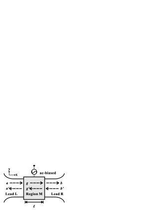
Figure 1: Schematic illustration of the quasi-1D spin-orbit quantum channel embedded in 2DEG. In this narrow channel, the electron gas has static Rashba and Dresselhaus spin-orbit interactions which are characterized by $\alpha_{0}$ and $\beta_{0}$ respectively. The central grey region, with width $l$, is biased by ac gate voltage so that Rashba strength locally modulated as $\alpha_{1}\cos(\omega t)$. The origin of $x$-axis is set at the left edge of the grey region.

The system under consideration is a two-dimensional electron gas (2DEG) that is present at the interface of a heterostructure due to modulation doping and has intrinsic static Rashba and Dresselhaus spin-orbit interactions. The system configuration is shown in Fig. 1. A quasi-one-dimensional (Q1D) narrow channel is formed from the 2DEG via a lateral confining potential (along the $y$ direction). The barrier separating the Q1D channel from the 2DEG should be strong enough so the tunneling time between them is much longer than the carrier transport time in the Q1D channel. A finger gate is placed in the middle of the channel (the grey region in Fig. 1) that modulates the local Rashba interaction strength sinusoidally via an ac-bias. Hence, the system can be described by the effective Hamiltonian

$$\hat{\mathcal{H}}=\frac{\hat{p}^{2}}{2m^{*}}+\hat{\mathcal{H}}^{\rm static}_{\mathrm{so}}+\hat{\mathcal{H}}_{\mathrm{so}}(\mathbf{r},t)+\hat{V}_{c}(y),$$ (1)

where $m^{*}$ denotes the electron effective mass and $\hat{V}_{c}(y)$ indicates the confinement potential in transverse ($y$) direction. $\hat{\mathcal{H}}^{\rm static}_{\mathrm{so}}$ and $\hat{\mathcal{H}}_{\mathrm{so}}(\mathbf{r},t)$ characterize, respectively, the static and dynamic parts of spin-orbit interaction. If we consider a narrow quantum channel where the subband energy spacing is large enough to decouple $\hat{p}_{y}$ from spin-orbit interaction, the intersubband mixing is thus neglected.Wang:5304 ; Tang:5804 The longitudinal part of the dimensionless Hamiltonian is then given by

$$\hat{\mathcal{H}}^{0}_{x} = \hat{k}_{x}^{2}-\alpha_{0}\sigma^{y}\hat{k}_{x}+\beta_{0}\sigma^{x}\hat{k}_{x},$$

$$\hat{\mathcal{H}}_{x}(t) = -\frac{1}{2}\alpha_{1}\sigma^{y}\cos(\omega t)\{\hat{k}_{x},\theta(l/2-|x-l/2|)\},$$ (2)

where $\sigma^{i}(i=\{x,y,z\})$ denotes Pauli matrices and $\hat{k}_{x}$ indicates the momentum operator $-i\partial_{x}$. Anticommutator $\{\cdots\}$ is used to maintain the hermitianity of $\hat{\mathcal{H}}_{x}(t)$. The static Rashba strength $\alpha_{0}$ is proportional the electric field perpendicular to the interface where 2DEG lies. Additionally, $\beta_{0}$ is the phenomenological Dresselhaus coupling parameter. In the finger gate region, the Rashba parameter oscillates sinusoidally with amplitude $\alpha_{1}$. For simplicity, we restrict the subsequent discussions to the lowest subband and ignore the subband index. The contributions from other subbands can be added if a more realistic consideration is needed.

To proceed, it is convenient to rotate the spin quantization axis such that $\hat{\mathcal{H}}^{0}_{x}$ is diagonalized. The transformed Hamiltonian is

$$\hat{\mathcal{H}}^{\prime 0}_{x} = \hat{k}_{x}^{2}-\gamma_{0}\sigma^{z}\hat{k_{x}},$$ (3)

$$\hat{\mathcal{H}}^{\prime}_{x}(t) = -\frac{1}{2}\alpha_{1}\sigma^{\phi}\cos(\omega t)\{\hat{k}_{x},\theta(l/2-|x-l/2|)\},$$ (4)

where $\sigma^{\phi}=(\sigma^{z}\sin\phi-\sigma^{y}\cos\phi)$, $\gamma_{0}=\sqrt{\alpha^{2}_{0}+\beta^{2}_{0}}$, and $\phi=\arctan(\alpha_{0}/\beta_{0})$. $\hat{\mathcal{H}}^{\prime 0}_{x}$ illustrates not only our choice of spin-up and spin-down states but also that the location of subband bottom is at $-\gamma^{2}_{0}/4$. Based on Floquet theorem, the wave functions in lead L ($x<0$) and lead R ($x>l$) are given by

$$\Psi^{L}(x,t) = \sum_{m,\sigma}(a_{m,\sigma}e^{ik^{R}_{m,\sigma}x}+a^{\prime}_{m,\sigma}e^{ik^{L}_{m,\sigma}x})e^{-i(\mu+m\omega)t}\chi_{\sigma},$$

$$\Psi^{R}(x,t) = \sum_{m,\sigma}(b_{m,\sigma}e^{ik^{R}_{m,\sigma}x}+b^{\prime}_{m,\sigma}e^{ik^{L}_{m,\sigma}x})e^{-i(\mu+m\omega)t}\chi_{\sigma},$$

where $\chi_{\sigma}$ denotes the spinor basis and $\mu$ represents the incident energy. The sideband index $m$ runs essentially for all integers. From the dispersion relation in Eq. (3$),k^{R}_{m,\sigma}$ and $k^{L}_{m,\sigma}$ are $\frac{1}{2}[\eta_{\sigma}\gamma_{0}+\sqrt{\gamma_{0}^{2}+4(\mu+m\omega)}]$ and $\frac{1}{2}[\eta_{\sigma}\gamma_{0}-\sqrt{\gamma_{0}^{2}+4(\mu+m\omega)}]$ respectively, where $\eta_{\sigma}$ is defined as $\sigma^{z}_{(\sigma,\sigma)}$. $a_{m,\sigma}$ ($a^{\prime}_{m,\sigma}$) is the amplitude of the rightward (leftward) wave in the mth sideband with spin $\sigma$ in lead L. Similarly, $b_{m,\sigma}$ ($b^{\prime}_{m,\sigma}$) is for lead R. Technically, these amplitudes are determined by boundary condition and the direction of incident wave.

In the time-dependent region M ($0<x<l$), the general solution would be

$$\Psi^{M}(x,t)=\sum_{m,\sigma}\Psi_{m,\sigma}(x)e^{-i(\varepsilon+m\omega)t}\chi_{\sigma},$$ (6)

where $\varepsilon$ is the Floquet quasi-energy. $\Psi_{m,\sigma}(x)$ is solved from Schrödinger’s equation,

$$\sum_{\sigma^{\prime}}[(\hat{k}_{x}^{2}-\gamma_{0}\hat{k}_{x}\sigma^{z}_{(\sigma,\sigma^{\prime})})\Psi_{m,\sigma^{\prime}} - \frac{\alpha_{1}\hat{k}_{x}}{2}\sigma^{\phi}_{(\sigma,\sigma^{\prime})}$$

$$(\Psi_{m+1,\sigma^{\prime}}+\Psi_{m-1,\sigma^{\prime}})] = (\varepsilon+m\omega)\Psi_{m,\sigma}.$$ (7)

These coupled equations can be expressed in matrix form,

$$\hat{k}_{x}^{2}\mathbf{\Psi}+\hat{k}_{x}\mathbf{H^{(1)}\Psi}=\mathbf{H^{(0)}\Psi},$$ (8)

where

$$\mathbf{H}^{\mathbf{(1)}}_{(m,\sigma)(m^{\prime},\sigma^{\prime})} = -\frac{\alpha_{1}}{2}\sigma^{\phi}_{(\sigma,\sigma^{\prime})}(\delta_{m,m^{\prime}+1}+\delta_{m,m^{\prime}-1})$$ (9)

$$-\gamma_{0}\sigma^{z}_{(\sigma,\sigma^{\prime})}\delta_{m,m^{\prime}},$$

$$\mathbf{H}^{\mathbf{(0)}}_{(m,\sigma)(m^{\prime},\sigma^{\prime})} = (\varepsilon+m\omega)\delta_{m,m^{\prime}}\delta_{\sigma,\sigma^{\prime}},$$ (10)

$$\mathbf{\Psi}_{m,\sigma} = \Psi_{m,\sigma}(x).$$ (11)

Because this is a transport problem, we have to solve the eigenvalue $q$ for fixed $\varepsilon$. This quadratic eigenproblem can be solved by introducing another of auxiliary equation $\mathbf{\Psi^{\prime}}=q\mathbf{\Psi}$. Then Eq. (8) becomes

$$\begin{pmatrix}\mathbf{0}&\mathbf{1}\\ \mathbf{H^{(0)}}&\mathbf{-H^{(1)}}\\ \end{pmatrix}\begin{pmatrix}\mathbf{\Psi}\\ \mathbf{\Psi^{\prime}}\\ \end{pmatrix}=q\begin{pmatrix}\mathbf{\Psi}\\ \mathbf{\Psi^{\prime}}\\ \end{pmatrix}.$$ (12)

If we truncate the sideband index $m$ at $-M/2$ and $M/2$, where $M$ is an even integer, the eigenvalues $q^{j}$ and eigenvectors $\psi^{j}_{m,\sigma}$ are numerically determined from the above secular equation.

Because Hamiltonian in Eq. (2) preserves time-reversal symmetry, any $q^{j}$ is associated with $-(q^{j})^{*}$, i.e. $\varepsilon(q^{j})=\varepsilon(-(q^{j})^{*})$. In addition, for Hamiltonian is also invariant under inversion followed by spin flip, $q^{j}$ has its another counterpart $-q^{j}$. Thus, we can definitely sort the $(4M+4)$ complex eigenvalues into two groups.

For the case of evanescent modes, those right-decaying waves are characterized by positive Im($q^{j}$); left-decaying waves have negative Im($q^{j}$). On the other hand, for the case of propagating modes that have real $q^{j}$, we sort $q^{j}$ with positive (negative) group velocity to be rightward (leftward) propagating waves. The group velocity is determined by $(d\varepsilon/dq^{j})$.Chan:0605 Therefore, the wave function in region M is given by

$$\Psi_{m,\sigma}(x)=\sum_{j}(g_{j}\psi^{j,R}_{m,\sigma}e^{iq^{j,R}x}+g^{\prime}_{j}\psi^{j,L}_{m,\sigma}e^{iq^{j,L}x}),$$ (13)

where superscripts $R$ and $L$ are added to indicate the propagating or decaying direction.

Wave functions are matched in the time domain by $\varepsilon$ = $\mu$ and continuous across the boundaries. Their derivatives satisfy the following boundary conditions:

$$\partial_{x}\Psi(x,t)|_{x=0^{+}}-\partial_{x}\Psi(x,t)|_{x=0^{-}} = \frac{i\alpha_{1}}{2}\cos(\omega t)\sigma^{\phi}\Psi(0,t),$$

$$\partial_{x}\Psi(x,t)|_{x=b^{-}}-\partial_{x}\Psi(x,t)|_{x=b^{+}} = \frac{i\alpha_{1}}{2}\cos(\omega t)\sigma^{\phi}\Psi(b,t).$$

The above boundary conditions can be written down in matrix form,

$$\mathbf{a+a^{\prime}} = \mathbf{S^{R}g+S^{L}g^{\prime}},$$ (15)

$$\mathbf{(K^{R}a+K^{L}a^{\prime})-(S^{R}Q^{R}g+S^{L}Q^{L}g^{\prime})} = \frac{1}{2}\mathbf{(\mathbf{H^{(1)}}-\gamma_{0}\mathbf{\Sigma})(a+a^{\prime})},$$ (16)

$$\mathbf{S^{R}}e^{i\mathbf{Q^{R}}l}\mathbf{g}+\mathbf{S^{L}}e^{i\mathbf{Q^{L}}l}\mathbf{g^{\prime}} = e^{i\mathbf{K^{R}}l}\mathbf{b}+e^{i\mathbf{K^{L}}l}\mathbf{b^{\prime}},$$ (17)

$$\mathbf{(K^{R}b+K^{L}b^{\prime})}-(\mathbf{S^{R}Q^{L}}e^{i\mathbf{Q^{R}}l}\mathbf{g}+\mathbf{S^{L}Q^{L}}e^{i\mathbf{Q^{L}}l}\mathbf{g^{\prime}}) = \frac{1}{2}\mathbf{(\mathbf{H^{(1)}}-\gamma_{0}\mathbf{\Sigma})}(e^{i\mathbf{K^{R}}l}\mathbf{b}+e^{i\mathbf{K^{L}}l}\mathbf{b^{\prime}}),$$ (18)

where those column vectors $\mathbf{a}$, $\mathbf{g}$, and $\mathbf{b}$, are assigned values from amplitudes $a_{m,\sigma}$, $g_{j}$, and $b_{m,\sigma}$ respectively. The above $(2M+2)\times(2M+2)$ matrices $\mathbf{S}^{\mathbf{R}(\mathbf{L})}$, $\mathbf{Q}^{\mathbf{R}(\mathbf{L})}$, $\mathbf{\Sigma}$, and $\mathbf{K}^{\mathbf{R}(\mathbf{L})}$ have matrix elements

$$\mathbf{S}^{\mathbf{R}(\mathbf{L})}_{(m,\sigma),j} = \psi^{j,R(L)}_{m,\sigma},$$

$$\mathbf{Q}^{\mathbf{R}(\mathbf{L})}_{j,j^{\prime}} = \delta_{j,j^{\prime}}q^{j,R(L)},$$

$$\mathbf{\Sigma}_{(m,\sigma)(m^{\prime},\sigma^{\prime})} = \delta_{m,m^{\prime}}\delta_{\sigma,\sigma^{\prime}}(-\delta_{\sigma,\uparrow}+\delta_{\sigma,\downarrow}),$$

$$\mathbf{K}^{\mathbf{R}(\mathbf{L})}_{(m,\sigma)(m^{\prime},\sigma^{\prime})} = \delta_{m,m^{\prime}}\delta_{\sigma,\sigma^{\prime}}(\delta_{\sigma,\uparrow}k^{R(L)}_{m,\uparrow}+\delta_{\sigma,\downarrow}k^{R(L)}_{m,\downarrow}).$$

After some algebra, we have the following matrix equation from Eqs. (15) to (18):

$$\begin{pmatrix}\mathbf{a^{\prime}}\\ \mathbf{b}\\ \end{pmatrix}=\begin{pmatrix}\mathcal{M}_{11}&\mathcal{M}_{12}\\ \mathcal{M}_{21}&\mathcal{M}_{22}\\ \end{pmatrix}\begin{pmatrix}\mathbf{a}\\ \mathbf{b^{\prime}}\\ \end{pmatrix}.$$ (20)

$\mathcal{M}=\begin{pmatrix}\mathcal{M}_{11}&\mathcal{M}_{12}\\ \mathcal{M}_{21}&\mathcal{M}_{22}\\ \end{pmatrix}$ denotes $(4M+4)\times(4M+4)$ matrix connecting the input coefficients with output coefficients including all propagating and evanescent Floquet sidebands.

In order to construct the Floquet scattering matrix, we need to introduce the concept of probability flux amplitude into $\mathcal{M}$. We can straightforward define a new matrix as

$$\mathcal{M}^{\prime}=\begin{pmatrix}\mathbf{V^{L}}&0\\ 0&\mathbf{V^{R}}\\ \end{pmatrix}\begin{pmatrix}\mathcal{M}_{11}&\mathcal{M}_{12}\\ \mathcal{M}_{21}&\mathcal{M}_{22}\\ \end{pmatrix}\begin{pmatrix}\mathbf{V^{R}}&0\\ 0&\mathbf{V^{L}}\\ \end{pmatrix}^{-1},$$ (21)

where $\mathbf{V}^{\mathbf{R(L)}}_{(m,\sigma)(m^{\prime},\sigma^{\prime})}=\delta_{m,m^{\prime}}\delta_{\sigma,\sigma^{\prime}}\sqrt{|2k^{R(L)}_{m,\sigma}-\eta_{\sigma}\gamma_{0}k^{R(L)}_{m,\sigma}|}$. In both leads, $\mathbf{V}^{\mathbf{R(L)}}$ takes the form of diagonal matrix with the square root of group velocity absolute value from each sideband and spin type. It is worth mention that $\mathcal{M}^{\prime}$ is not unitary yet due to the presence of evanescent modes. In the final stage, we obtain a unitary Floquet scattering matrix by setting the evanescent modes of the total scattering matrix $\mathcal{M}^{\prime}$ to be zero:

$$\mathcal{S}=\begin{pmatrix}{\mathcal{R}}&{\mathcal{T^{\prime}}}\\ {\mathcal{T}}&{\mathcal{R^{\prime}}}\\ \end{pmatrix}.$$ (22)

The unitarity of Floquet scattering matrix reflects the current conservation law,Li:5732 ; Hens:6218 and is used as the criteria to check numerical convergence.

The reflection and transmission coefficients are readily obtained by summing over matrix elements of $\mathcal{S}$. When electrons that are incident from L lead with initial spin $\sigma_{i}$ are partially reflected and transmitted to final spin $\sigma_{f}$, the spin-resolved reflection and transmission coefficients are written as

$$R_{\sigma_{f}\sigma_{i}}^{LL}(\varepsilon) = \sum_{m}|{\mathcal{R}}_{(m,\sigma_{f})(0,\sigma_{i})}|^{2},$$ (23)

$$T_{\sigma_{f}\sigma_{i}}^{RL}(\varepsilon) = \sum_{m}|{\mathcal{T}}_{(m,\sigma_{f})(0,\sigma_{i})}|^{2}.$$ (24)

On the contrary, if the electron is incident from lead R, this gives rise to such reflection and transmission coefficients

$$R_{\sigma_{f}\sigma_{i}}^{RR}(\varepsilon) = \sum_{m}|{\mathcal{R^{\prime}}}_{(m,\sigma_{f})(0,\sigma_{i})}|^{2},$$ (25)

$$T_{\sigma_{f}\sigma_{i}}^{LR}(\varepsilon) = \sum_{m}|{\mathcal{T^{\prime}}}_{(m,\sigma_{f})(0,\sigma_{i})}|^{2}.$$ (26)

Under zero longitudinal bias, the spin-resolved current pumped out through lead R is generally defined as

$$I^{R}_{\uparrow} = \frac{e}{h}\int d\varepsilon f(\varepsilon)[T_{\uparrow\uparrow}^{RL}+T_{\uparrow\downarrow}^{RL}+R_{\uparrow\uparrow}^{RR}+R_{\uparrow\downarrow}^{RR}-1],$$

$$I^{R}_{\downarrow} = \frac{e}{h}\int d\varepsilon f(\varepsilon)[T_{\downarrow\uparrow}^{RL}+T_{\downarrow\downarrow}^{RL}+R_{\downarrow\uparrow}^{RR}+R_{\downarrow\downarrow}^{RR}-1],$$

where $f(\varepsilon)$ is Fermi-Dirac distribution. The spin-resolved current can be derived based on the framework of Büttiker’s formulaButt:2485 by regarding two spin types as different terminal channels. The generalization of Büttiker’s formula for Floquet scattering matrix has been strictly proven.Levi:1399 ; Kim:3309 The spin current and charge current at lead R are defined as $I_{s}^{R}=I^{R}_{\uparrow}-I^{R}_{\downarrow}$ and $I_{c}^{R}=I^{R}_{\uparrow}+I^{R}_{\downarrow}$. Because system Hamiltonian in Eq. (2) has inversion followed by spin flip symmetry, we can transform the transmission and reflection coefficients as $T_{\sigma_{f}\sigma_{i}}^{LR}=T_{-\sigma_{f}-\sigma_{i}}^{RL}$ and $R_{\sigma_{f}\sigma_{i}}^{RR}=R_{-\sigma_{f}-\sigma_{i}}^{LL}$. Such transformation firstly guaranteed that there is zero charge current in this system. Secondly, when certain amount of spin current is pumped out at lead R, there should be equal amount of spin current with opposite polarization pumped out at lead L. Furthermore, if this symmetry is combined with current conservation condition, spin current formula can be simplified to a more convenient form in calculation:

$$I^{R}_{s}=\frac{2e}{h}\int d\varepsilon f(\varepsilon)[(T_{\uparrow\uparrow}^{RL}-T_{\downarrow\downarrow}^{RL})+(R_{\uparrow\downarrow}^{RR}-R_{\downarrow\uparrow}^{RR})].\\$$ (28)

The first two terms represent contributions from transmitted electrons, and the last two terms are attributed to reflected electrons whose spin is changed. Hence, we separate $I^{R}_{s}$ into spin-preserved transmission and spin-flip reflection parts because their effects are different and discussed in the following context. Thus,

$$I^{R}_{s}=I^{R,{\rm trans}}_{s}+I^{R,{\rm refl}}_{s}.$$ (29)

It should be noted that if there is no Dresselhaus term, the $I^{R,{\rm refl}}_{s}$ term is identically zero, and the $I^{R}_{s}$ is then reduced to the same form in Ref. Wang:5304, .

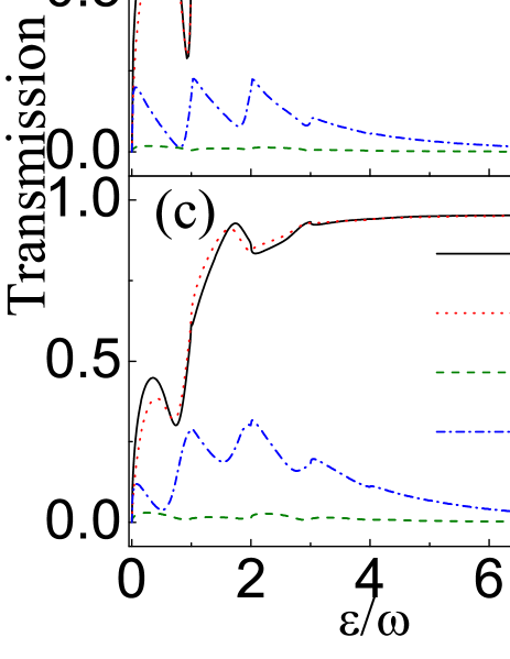
Figure 2: Spin-resolved transmission and reflection coefficients $T_{\uparrow\uparrow}^{RL}$, $T_{\downarrow\downarrow}^{RL}$, $R_{\uparrow\downarrow}^{RR}$, and $T_{\downarrow\uparrow}^{RR}$ as functions of the incident energy. The values of reflection coefficients are multiplied by 50 to clarify the shape of the curves. $\alpha_{0}=0.12$, $\beta_{0}=\alpha_{0}$, $l=30$, $\omega=0.002$, and $\alpha_{1}=$(a) $0.04$, (b) $0.06$, (c) $0.08$. The spin current, $I_{s}^{R}$, which depend on Fermi energy for different $\alpha_{1}$ are plotted in (d).

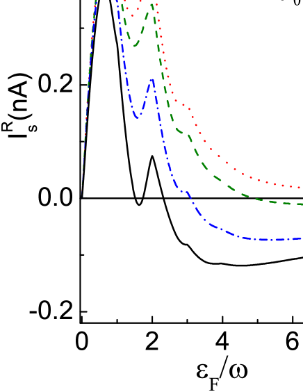
Figure 3: (a) Pumped spin current $I_{s}^{R}$ the Fermi energy (related to the bottom of the first subband in Q1D channel). $\beta_{0}$ is 0, 0.03, 0.06, and 0.12. Parameters $\alpha_{1}=0.08$, $\alpha_{0}=0.12$, $l=30$, and $\omega=0.002$. (b)$I^{R}_{s}$, $I^{R,{\rm trans}}_{s}$, and $I^{R,{\rm refl}}_{s}$ are illustrated for $\beta_{0}=0.12$ case in (a).

III Results and discussion

Utilizing the above derived formula in previous section, it is easy to calculate the spin current pumped from the spin-orbit quantum channel via numerical means. The reasonable material parameters are chosen from the narrow-gap heterostructure based on InGaAs-InAlAs based system. According the experimental data, we assume that the 2DEG has an electron density $n_{e}=1\times 10^{12}$ $\mathrm{cm}^{-2}$, effective mass $m^{*}=0.04m_{0}$, and $\alpha_{0}=0.12$ ($\hbar\alpha_{0}=2.8\times 10^{-11}$ eV m).Nitt:1335 The ratio between Rashba and Dresselhaus terms can vary in certain range due to experimental difficulties.Gigl:5327 Thus, we examine the cases for $\beta_{0}/\alpha_{0}$ varying between 0 and 1. In our calculations, the length and energy units are chosen to be $l^{*}=4.0$ nm and $E^{*}=59$ meV (the Fermi energy of the 2DEG). We assume that the ac-biased gate has a width of $l=30l^{*}$ and its driving frequency is chosen as $\hbar\omega=0.002E^{*}$ ($\omega/2\pi=28$ GHz). The bottom of the lowest energy level (first subband) in the Q1D channel is assumed to be slightly below the Fermi level, $E^{*}$ of the 2DEG so that the Fermi energy relative to the bottom of the first subband in the Q1D channel (denoted $\varepsilon_{F}$) is comparable to $\hbar\omega$. All numerical results are obtained for zero temperature.

The dependence of transmission and reflection coefficients on the incident electron energy ($\varepsilon$) for various values of $\alpha_{1}$ are illustrated in Figs. 2(a)-(c) when the static Rashba and Dresselhaus constants are the same, i.e. $\beta_{0}=\alpha_{0}$. In order to clarify the important features shown in these figures, we redefine the energy zero at the bottom of the first subband with the presence of Rashba and Dresselhaus terms, i.e. $\hat{\mathcal{H}}^{\prime 0}_{x}\rightarrow\hat{\mathcal{H}}^{\prime 0}_{x}+\gamma_{0}^{2}/4$. The coefficients $T_{\uparrow\uparrow}^{RL}$, $T_{\downarrow\downarrow}^{RL}$, $R_{\uparrow\downarrow}^{RR}$, and $R_{\downarrow\uparrow}^{RR}$, which are needed for calculating $I^{R}_{s}$, are plotted in Figs. 2(a)-(c). For transmission coefficients, we find sharp features at integer values of $\varepsilon/\omega$, indicative of the resonant inelastic scattering. As $\alpha_{1}$ increases, the dip around $\varepsilon/\omega=1$ moves toward lower energy, and the dip width is broadened. The reason for the shift of dip location is that a stronger oscillating potential would lower the real part of the quasi-bound state energy and shorten the lifetime of electrons trapped in such a state.Li:5732 When $\alpha_{1}$ is increased to 0.08 as shown in Fig. 2(c), a higher order resonance seen as a shallow dip around $\varepsilon/\omega=2$ becomes more apparent because of the absorption and emission of two quanta (with energy $2\hbar\omega$). The most significant effect of the Dresselhaus interaction is the emergence of the spin-flip process, which leads to appreciable spin-flip reflection coefficients, $R_{\uparrow\downarrow}^{RR}$ and $R_{\downarrow\uparrow}^{RR}$. In Figs. 2(a)-2(c), $R_{\uparrow\downarrow}^{RR}$ and $R_{\downarrow\uparrow}^{RR}$ have a saw-like behavior with peaks appearing at integer values of $\varepsilon/\omega$, where electrons are bounced back due to the presence of quasi-bound states. Although their values are still minute compared with $T_{\uparrow\uparrow}^{RL}$ and $T_{\downarrow\downarrow}^{RL}$, they can lead to significant change in the final spin current when we take differences of the spin-up and spin-down contributions.

Figure 2(d) illustrates the spin current as a function of the Fermi energy, $\varepsilon_{F}$ (which reflects the carrier density in the Q1D channel) for various values of $\alpha_{1}$. The curves in this Figs 2(a)-(c) can be approximately divided into two parts: the low energy region ($\varepsilon/\omega<2$) and high energy region ($\varepsilon/\omega>2$). In the low energy region, the reflection coefficients are too small compared to $(T_{\uparrow\uparrow}^{RL}-T_{\downarrow\downarrow}^{RL})$, and $I^{R}_{s}$ is dominated by the contribution due to transmission process (denoted $I^{R,{\rm trans}}_{s}$). In the high energy region, $(R_{\uparrow\downarrow}^{RR}-R_{\downarrow\uparrow}^{RR})$ becomes stronger than $(T_{\uparrow\uparrow}^{RL}-T_{\downarrow\downarrow}^{RL})$ and the contribution to $I^{R}_{s}$ due to reflection process (denoted $I^{R,{\rm refl}}_{s}$) becomes dominant. As $\alpha_{1}$ increases from 0.04 to 0.06, more spin current is pumped out the first peak at $\varepsilon_{F}/\omega=1$ and into the second peak at $\varepsilon_{F}/\omega=2$. When $\alpha_{1}$ is tuned even higher to 0.08, high order resonances become more relevant. Thus we have a further enhanced peak around $\varepsilon_{F}/\omega=2$ and a reduced peak around $\varepsilon_{F}/\omega=1$. However, because $(R_{\uparrow\downarrow}^{RR}-R_{\downarrow\uparrow}^{RR})$ is always negative, $I^{R,{\rm refl}}_{s}$ results in negative contribution to $I^{R}_{s}$ and it pulls the spin current curves downward. For $\varepsilon_{F}/\omega>2$, $I^{R,{\rm refl}}_{s}$ becomes dominant so that negative spin current is generated. As $\alpha_{1}$ increases, $I^{R}_{s}$ (for $\varepsilon_{F}/\omega>2$) becomes more negative due to higher probability of the spin-flip process.

In Fig. 3(a), we focus on the effect of Dresselhaus interaction on the pumped spin current for a fixed $\alpha_{1}$. In the case of zero $\beta_{0}$, only one kind of spin polarization can be pumped.Wang:5304 As $\beta_{0}$ increases, $I^{R}_{s}$ curves tend to shift downward due to increased spin-flip scattering process. In the low density case ($\varepsilon_{F}/\omega<2$), experimentally reasonable $\beta_{0}$ may hardly change the sign of $I_{s}^{R}$. In the higher density case ($\varepsilon_{F}/\omega>2$), the sign of $I^{R}_{s}$ is more vulnerable to the strength of the Dresselhaus term. When $\beta_{0}$ is 0.03, 0.06, and 0.12, the threshold values of $\varepsilon$ at which the sign of $I^{R}_{s}$ starts to change are at $\varepsilon_{F}/\omega$ = 4.89, 3.09, and 2.32, respectively.

A simple physical picture is presented here to give a conclusive explanation. The conditions in Fig. 3(b) are taken as an example. Based on the dispersion relation of $\hat{\mathcal{H}}^{\prime 0}_{x}$ in Eq. (3), when the electron is incident from lead L, $|k^{R}_{0,\uparrow}|$ is always larger than $|k^{L}_{0,\downarrow}|$ for the same energy. Thus, it is easier for spin-up electron to tunnel through this oscillating barrier due its larger flux, i.e. this dispersion of static Hamiltonian tends to favor $T_{\uparrow\uparrow}^{RL}$ rather than $T_{\downarrow\downarrow}^{RL}$. On the other hand, because scattering potential $\hat{\mathcal{H}}^{\prime 1}_{x}$ can be approximately regarded as proportional to momentum, spin-up electrons could be more susceptible to the scattering process so that $T_{\downarrow\downarrow}^{RL}$ is favored here. In low energy region, these two mechanisms are competing so that $(T_{\uparrow\uparrow}^{RL}-T_{\downarrow\downarrow}^{RL})$ may be positive or negative and $I^{R,{\rm trans}}_{s}$ has obvious peaks.

In high energy region, because the second mechanism is less relevant, only monotonically increasing $I^{R,{\rm trans}}_{s}$ is present. For $I^{R,{\rm refl}}_{s}$, the situation is just on the opposite side. Because $|k^{L}_{0,\downarrow}|$ is greater than $|k^{L}_{0,\uparrow}|$, there would be less chance for incident spin-down electrons to be reflected. Hence, $I^{R,{\rm refl}}_{s}$ always contributes to negative spin current and is monotonically decreasing. When incident energy is low, $I^{R,{\rm refl}}_{s}$ only compensates part of $I^{R,{\rm trans}}_{s}$. When energy increases, $I^{R,{\rm refl}}_{s}$ becomes dominant and there is a threshold $\varepsilon/\omega$ beyond which $I^{R}_{s}$ starts to change sign.

IV conclusion

We have proposed a promising approach to generate spin current non-magnetically in the absence of charge current. A quasi-1D channel with static Rashba and Dresselhaus spin orbit interaction is studied. Spin pumping is achieved by an ac gate voltage to locally modulate the Rashba constant. Pumped spin current can be attributed to both the spin-preserved transmission and the spin-flip reflection processes. These two terms contribute to opposite polarization of the spin current.

It is found that in the low density case ($\varepsilon_{F}/\omega<2$), the spin-preserved transmission is dominant and featured by resonant inelastic scattering. In the high density case ($\varepsilon_{F}/\omega>2$), there is a threshold beyond which spin current begins to switch polarization. Furthermore, it is found that the static Dresselhaus coefficient $\beta_{0}$ as well as the dynamic Rashba coefficient $\alpha_{1}$ can enhance the spin-flip process and modify the threshold value of $\varepsilon_{F}/\omega$, at which the spin polarization switches. In conclusion, we have demonstrated a feasible way to control dynamically the intensity and polarization of the spin current via changing the strength of the ac-biased gate voltage and tuning the driving frequency.

References

• (1) G. A. Prinz, Science 282, 1660 (1998); S. A. Wolf, D. D. Awschalom, R. A. Buhrman, J. M. Daughton, S. von Molnar, M. L. Roukes, A. Y. Chtchelkanova, and D. M. Treger, ibid. 294, 1488 (2001); Y. Kato, R. C. Myers, D. C. Driscoll, A. C. Gossard, J. Levy, D. D. Awschalom, ibid. 294, 148 (2001).
• (2) I. Zutic, J. Fabian, and S. Das Sarma, Rev. Mod. Phys, 76, 323 (2004).
• (3) G. Burkard, D. Loss, and D. P. DiVincenzo, Phys. Rev. B 59, 2070 (1999).
• (4) S. K. Watson, R. M. Potok, C. M. Marcus, and V. Umansky, Phys. Rev. Lett. 91, 258301 (2003).
• (5) Q. F. Sun, H. Guo, and J. Wang, Phys. Rev. Lett. 90, 258301 (2003).
• (6) P. Zhang, Q. K. Xue, and X. C. Xie, Phys. Rev. Lett. 91, 196602 (2003).
• (7) A. Brataas1, Y. Tserkovnyak, G. E. W. Bauer, and B. I. Halperin, Phys. Rev. B 66, 060404(R) (2002).
• (8) P. Sharma, Science 307, 531 (2005).
• (9) C. Li, Y. Yu, Y. Wei, and J. Wang, Phys. Rev. B 75, 035312 (2007).
• (10) D. J. Thouless, Phys. Rev. B 27, 6083 (1983).
• (11) P. W. Brouwer, Phys. Rev. B 58, R10135 (1998).
• (12) M. Switkes, C. M. Marcus, K. Campman, and A. C. Gossard, Science 283, 1905 (1999).
• (13) C. S. Tang and C. S. Chu, Solid State Communications 120, 353 (2001).
• (14) B. Wang, J. Wang, and H. Guo, Phys. Rev. B 65, 073306 (2002).
• (15) M. G. Vavilov, V. Ambegaokar, and, I. L. Aleiner, Phys. Rev. B 63, 195313 (2001).
• (16) E. R. Mucciolo, C. Chamon, and C. M. Marcus, Phys. Rev. Lett. 89, 146802 (2002).
• (17) R. Benjamin and C. Benjamin, Phys. Rev. B 69, 085318 (2004).
• (18) M. Governale, F. Taddei, and R. Fazio, Phys. Rev. B 68, 155324 (2003).
• (19) L. Y. Wang, C. S. Tang, and C. S. Chu , Phys. Rev. B 73, 085304 (2006).
• (20) C. S. Tang and Y. C. Chang, arXiv:cond-mat/0611703v1.
• (21) G. Dresselhaus, Phys. Rev. 100, 580 (1955).
• (22) L. Zhang, P. Brusheim, and H. Q. Xu, Phys. Rev. B 72, 045347 (2005).
• (23) B. H. Wu and J. C. Cao, Phys. Rev. B 73, 245412 (2006).
• (24) Y. C. Chang, Phys. Rev. B 25, 605 (1982).
• (25) W. Li and L. E. Reichl, Phys. Rev. B 60, 15732 (1999).
• (26) M. Henseler1, T. Dittrich, and K. Richter, Phys. Rev. E 64, 046218 (2001).
• (27) M. Büttiker, Phys. Rev. B 48, 12485 (1992).
• (28) Y. Levinson and P. Wölfle, Phys. Rev. Lett. 83, 1399 (1999).
• (29) S. W. Kim, Phys. Rev. B 68, 033309 (2003).
• (30) J. Nitta, T. Akazaki, H. Takayanagi, and T. Enoki, Phys. Rev. Lett. 78, 1335 (1997).
• (31) S. Giglberger, L. E. Golub, V. V. Bel kov, S. N. Danilov, D. Schuh, C. Gerl, F. Rohlfing, J. Stahl, W. Wegscheider, D. Weiss, W. Prettl, and S. D. Ganichev, Phys. Rev. Lett. 75, 035327 (2007).