A General Theory of Computational Scalability Based on Rational Functions

Abstract

The universal scalability law of computational capacity is a rational function $C_{p}=P(p)/Q(p)$ with $P(p)$ a linear polynomial and $Q(p)$ a second-degree polynomial in the number of physical processors $p$, that has been long used for statistical modeling and prediction of computer system performance. We prove that $C_{p}$ is equivalent to the synchronous throughput bound for a machine-repairman with state-dependent service rate. Simpler rational functions, such as Amdahl’s law and Gustafson speedup, are corollaries of this queue-theoretic bound. $C_{p}$ is further shown to be both necessary and sufficient for modeling all practical characteristics of computational scalability.

1 Introduction

For several decades, a class of real functions called rational functions [ratfuns ], has been used to represent throughput scalability as a function of physical processor configuration. In particular, Amdahl’s law [amdahl ], its modification due to Gustafson [gusto ] and the Universal Scalability Law (USL) [cmg93 ] have found ubiquitous application. In this context, the relative computing capacity, $C_{p}$, is a rational function of the number of physical processors $p$. It is defined as the quotient of a polynomial $P(p)$ in the numerator and $Q(p)$ in the denominator, i.e., $C_{p}=P(p)/Q(p)$. Each of the above-mentioned scalability models is distinguished by the number of coefficients or fitting parameters associated with the polynomials in $P(p)$ and $Q(p)$. For example, Amdahl’s law and Gustafson’s modification are single parameter models, whereas the USL model contains two parameters.

Despite their historical utility, these models have stood in isolation without any deeper physical interpretation. It has even been suggested that Amdahl’s law is not fundamental [prep ]. More importantly, the lack of a unified physical interpretation has led to the use of certain flawed scalability models [arxiv02 ]. In this note, we demonstrate that the aforementioned class of rational functions corresponds to certain performance bounds belonging to a queue-theoretic model.

The idea that Amdahl’s law, which has most frequently been associated with the scalability of massively parallel systems, can be considered from a queue-theoretic standpoint, is not entirely new [See e.g., kleinrock92 , nelson ]. However, quite apart from motivations entirely different from our own, those previous works employed open queueing models with an unbounded number of requests (See Appendix C), whereas we shall use a closed queueing model with a finite number of requests $p$ corresponding to the number of physical processors. The USL function is associated with a state-dependent generalization of the machine repairman [ipl ].

The organization of this paper is as follows. We briefly review the scalability models of interest in Sect. 2. The appropriate queueing metrics associated with the standard machine repairman and its state-dependent extension are discussed in Sect. 3. The performance characteristics associated with synchronous queueing are also presented there. The main theorem (Theorem 2) is established in Sect. 4. Amdahl’s law and Gustafson’s linear speedup are shown to be corollaries of this theorem. Finally, in Sect. 5 we prove an earlier conjecture that a rational function with $Q(p)$ a second-degree polynomial is both necessary and sufficient to model all practical cases of computational scalability.

2 Parametric Models

Although technically, we are discussing rational functions, we shall hereafter refer to them as parametric models, and the coefficients as parameters, since the primary application of these models is nonlinear statistical regression of performance data [See e.g., cmg93 , gcap , pdcs , zone , and references therein].

Figure 1: Parametric models: USL (red), Amdahl (green), Gustafson (blue), with parameter values exaggerated to distinguish their typical characteristic relative to ideal linear scaling (dashed). The horizontal line is the Amdahl asymptote at $\sigma^{-1}$

.

Definition 1 (Speedup).

If an amount of work $N$ is completed in time $T_{1}$ on a uniprocessor, the same amount of work can be completed in time $T_{p}<T_{1}$ on a $p$-way multiprocessor. The speedup $S_{p}=T_{1}/T_{p}$ is one measure of scalability.

2.1 Amdahl’s law

For a single task that takes time $T_{1}$ to execute on a uniprocessor ($p=1$), Amdahl’s law [amdahl ] states that if the task can be equipartitioned onto $p$ processors, but contains an irreducible fraction of sequential work $\sigma\in[0,1]$, then only the remaining portion of the execution time $(1-\sigma)T_{1}$ can be executed as $p$ parallel subtasks on $p$ physical processors. The bound on the achievable equipartitioned speedup [ware ] is given by the ratio

$$S_{p}(\sigma)=\dfrac{T_{1}}{\sigma T_{1}+\biggl{(}\dfrac{1-\sigma}{p}\biggr{)}T_{1}}$$ (1)

which simplifies to

$$S_{p}(\sigma)=\dfrac{p}{1+\sigma(p-1)}\,;$$ (2)

a rational function with $P(p)=p$ and $Q(p)$ a first-degree polynomial. As the processor configuration is increased, i.e., $p\rightarrow\infty$, the number of concomitantly smaller subtasks also increases and the speedup (1) approaches an asymptote,

$$S_{p}(\sigma)\sim\sigma^{-1}\,,$$ (3)

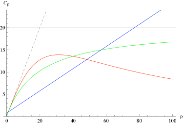
shown as the horizontal in Fig. 1.

2.2 Gustafson’s speedup

Amdahl’s law assumes the size of the work is fixed. Gustafson’s modification is based on the idea of scaling up the size of the work to match $p$. This assumption results in the theoretical recovery of linear speedup

$$S^{G}_{p}(\sigma)=\sigma+(1-\sigma)p$$ (4)

Equation (4) is a rational function with $Q(p)=1$ and $P(p)$ a first-degree polynomial in $p$.

Although (4) has inspired various efforts for improving parallel processing efficiencies, achieving truly linear speedup has turned out to be difficult in practice. Most recently, (4) has been proposed as a way to optimize the throughput of multicore processors [sutter ].

Definition 2 (Relative Capacity).

As an alternative to the speedup, scalability can also be defined as the relative capacity, $C_{p}=X(p)/X(1)$, where $X(p)$ is the throughput with $p$ processors, and $X(1)$ the throughput of a single processor.

2.3 Universal Scalability Law (USL)

The USL model [cmg93 , pdcs , gcap ] is a rational function with $P(p)=p$ and $Q(p)$ a second-degree polynomial:

$$C_{p}(\sigma,\kappa)=\dfrac{p}{1+\sigma(p-1)+\kappa\,p(p-1)}$$ (5)

where the coefficients belonging to the terms in the denominator have been regrouped into three terms with two parameters $(\sigma,\kappa)$. These terms can be interpreted as representing:

1. Ideal concurrency associated with linear scalability ($\sigma,\kappa=0$)

2. Contention-limited scalability due to serialization or queueing ($\sigma>0,\kappa=0$)

3. Coherency-limited scalability due to inconsistent copies of data ($\sigma,\kappa>0$)

Table 1 summarized how these parameter values can be used to classify the scalability of different types of applications.

Equation (5) subsumes (2) and (4). In particular, (2) is identical to (5) with $\kappa=0$. The key distinction is that, unlike (2), (5) possesses a maximum at

$$p^{*}=\sqrt{\dfrac{1-\sigma}{\kappa}}$$ (6)

which is controlled by the parameter values according to:

1. $p^{*}\rightarrow 0$ as $\kappa\rightarrow\infty$

2. $p^{*}\rightarrow\infty$ as $\kappa\rightarrow 0$

3. $p^{*}\rightarrow\kappa^{-1/2}$ as $\sigma\rightarrow 0$

4. $p^{*}\rightarrow 0$ as $\sigma\rightarrow 1$

The important implication is that beyond $p^{*}$ the throughput becomes retrograde. See Fig. 1. This effect is commonly observed in applications that involve shared-writable data (Case D in Table 1).

In the subsequent sections, we attempt to provide deeper insight into the physical significance of (5) by recognizing its association with queueing theory.

Table 1: Application domains for the USL model

A: Ideal concurrency ($\sigma,\kappa=0$)	B: Contention-limited ($\sigma>0,\kappa=0$)
Single-threaded tasks	Tasks requiring locking or sequencing
Parallel text search	Message-passing protocols
Read-only queries	Polling protocols (e.g., hypervisors)
C: Coherency-limited ($\sigma=0,\kappa>0$)	D: Worst case ($\sigma,\kappa>0$)
SMP cache pinging	Tasks acting on shared-writable data
Incoherent application state between	Online reservation systems
cluster nodes	Updating database records

3 Queueing Models

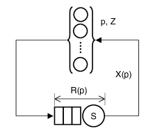
The machine repairman (Fig. 2) is a well-known queueing model [gross ] which represents an assembly line comprising a finite number of machines $p$ which break down after a mean lifetime $Z$. A repairman takes a mean time $S$ to repair a broken machine and if multiple machines fail, the additional machines must queue for service in FIFO order. The queue-theoretic notation, $M/M/1//p$, implies exponentially distributed lifetimes and service periods with a finite population $p$ of requests and buffering.

Figure 2: Conventional machine repairman queueing model comprising $p$ machines with mean uptime $Z$ (top) and a repair queue (bottom) with mean service time $S$.

3.1 Queueing Metrics

The performance characteristics of interest for the subsequent discussion are the throughput $X(p)$ and residence time $R(p)$.

Definition 3 (Throughput).

The throughput, $X=N/T$, is the number of tasks $N$ completed in time $T$.

Definition 4 (Residence Time).

The mean residence time $R=W+S$ is the sum of the time spent waiting for service $W$ plus the actual repair time $S$ when the repairman services the machine.

On average, the number of machines that are “up” is $ZX$, while $Q$ are “down” (for repairs), such that the total number of machines in either state is given by $p=Q+ZX$. Rearranging this expression produces:

$$Q=p-ZX$$

and applying Little’s law [gross ] ($Q=XR$) [gross ]

$$XR=p-ZX$$

gives

$$R(p)=\dfrac{p}{X(p)}-Z$$ (7)

for the mean residence time at the repair station. Rearranging (7) provides an expression for the mean throughput of the repairman as a function of $p$:

$$X(p)=\dfrac{p}{R(p)+Z}$$ (8)

Definition 5 (Mean RTT).

The denominator in (8), $R(p)+Z$, is the mean round-trip time (RTT) for $M/M/1//p$.

Table 2: Interpretation of the queueing metrics in Fig. 2

	Interpretation
Metric	Repairman	Multiprocessor	Time share
p	machines	processors	users
Z	up time	execution period	think time
S	service time	transmission time	CPU time
R(p)	residence time	interconnect latency	run-queue time
X(p)	failure rate	bandwidth	throughput

Since $M/M/1//p$  is an abstraction, it can be applied to different computational contexts. In the subsequent sections, the $p$ machines will be taken to represent physical processors and the time spent at the repair station is taken to represent the interconnect latency between the processors [reed , balbo ]. See Table 2. This choice is merely to conform to the conventions most commonly used in discussions of parallel scalability [pdcs ], but the generic nature of queueing model means that any conclusions also hold for software scalability [See e.g., gcap , Chap. 6].

3.2 Synchronous Queueing

We consider the special case of synchronous queueing in $M/M/1//p$. The queue-theoretic performance metrics defined in Sect. 3.1 are for the steady-state case and therefore each corresponds to the statistical mean of the respective random variable. Moreover, as already mentioned, we cannot give an explicit expression for $R(p)$ since its value is dependent on the value of $X(p)$, which is also unknown in steady state.

Definition 6 (Synchronized Requests).

If all the machines in $M/M/1//p$ break down simultaneously, the queue length at the repairman is maximized such that the residence time in definition 4 becomes $R(p)=pS$. This situation corresponds to one machine in service and $(p-1)$ waiting for service and provides a lower bound on (8) [muntz1 , bb , muntz2 ]:

$$\dfrac{p}{pS+Z}\leq X(p)$$ (9)

In the context of multiprocessor scalability (Table 2), it is tantamount to all $p$ processors simultaneously issuing requests across the interconnect.

Remark 1 (A Paradox).

Consider the case where all $p$ processors have the same deterministic $Z$ period. At the end of the first $Z$ period, all $p$ requests will enqueue at the interconnect (lower portion of Fig. 2) simultaneously. By definition, however, the requests are serviced serially, so they will return to the parallel execution phase (top portion of Fig. 2) separately and thereafter will always return to the interconnect at different times. In other words, even if the queueing system starts with synchronized visits to the interconnect, that synchronization is immediately lost after the first tour because it is destroyed by the serial queueing process. The resolution of this paradox is discussed in Appendix B.

Definition 7 (Synchronous RTT).

In the presence of synchronous queueing, the mean RTT of definition 5 becomes $pS+Z$.

Lemma 1.

The relative capacity $C_{p}$ and the speedup $S_{p}$ give identical values for the same processor configuration $p$.

Proof.

Let the uniprocessor throughput is defined as $X_{1}=N/T_{1}$ and the multiprocessor throughput is $X_{p}=N/T_{p}$. Hence

$$C_{p}=\dfrac{X(p)}{X(1)}=\dfrac{N}{T_{p}}\dfrac{T_{1}}{N}\equiv S_{p}$$

follows from definition 1. ∎

Lemma 2 (Serial Fraction).

The serial fraction (2.1) can be expressed in terms of $M/M/1//p$  metrics by the identity [arxiv02 , pdcs , gcap ]:

$$\sigma=\dfrac{S}{S+Z}\rightarrow\begin{cases}0&\text{as $S\rightarrow 0,\;Z=$ const.},\\ 1&\text{as $Z\rightarrow 0,\;S=$ const}.\end{cases}$$ (10)

If $\sigma=0$, then there is no communication between processors and the interconnect latency therefore vanishes (maximal execution time). Conversely, if $\sigma=1$, then the execution time vanishes (maximal communication latency).

Proof.

The RTT for a single (unpartitioned) task in Fig. 2 is $T_{1}=S+Z$. The RTT for a $p$ equipartitioned subtasks is $T_{p}=p(S/p)+Z/p$. From definition 1, the corresponding speedup is

$$S_{p}=\dfrac{S+Z}{S+Z/p}$$ (11)

Equating (11) with (1), we find

$$S=\sigma T_{1}\quad\text{and}\quad Z=(1-\sigma)T_{1}\,.$$ (12)

Eliminating $T_{1}$ produces

$$S=\biggl{(}\dfrac{\sigma}{1-\sigma}\biggr{)}Z$$ (13)

which, upon solving for $\sigma$, produces (10). ∎

See Appendix B for another perspective.

Definition 8.

The quantity

$$\frac{Z}{S}=\frac{1-\sigma}{\sigma}$$ (14)

is the service ratio for the $M/M/1//p$  model.

Theorem 1 (Speedup Duality).

Let $(\sigma,\pi)$ be a continuous dual-parameter pair with $\sigma$ is the serial fraction (10) and $\pi=1-\sigma$. The Amdahl speedup (2) is invariant under scalings of $(\sigma,\pi)$ by $p$.

Proof.

Using definition 8, theorem 1 can be represented diagrammatically as:

$$\begin{matrix}&&\pi/\sigma=Z/S&&\\ &\swarrow&&\searrow&\\ Z\mapsto Z/p&&&&Z\mapsto Z\\ S\mapsto S&&&&S\mapsto pS\\ &\searrow&&\swarrow&\\ &&S_{p}(\sigma)&&\\ \end{matrix}$$ (15)

The path on the left hand side of (15) corresponds to reducing the single task execution time by $p$ (subtasks) while the interconnect service time remains unchanged. This follows from definition 6, $R=pS$, but the service time for each subtask is also reduced to $S/p$. Hence, $R=S$. Conversely, the right hand path of (15) corresponds to $p$ tasks, each with unchanged execution time $Z$, but scaled service time $R=pS$. Both paths result in Amdahl’s law (2), which can be seen by first rewriting (11) in terms of the service ratio $Z/S$ (definition 8):

$$S_{p}=\dfrac{1+Z/S}{1+\dfrac{1}{p}\biggl{(}\dfrac{Z}{S}\biggr{)}}\,.$$ (16)

1. Interpreting the denominator in (16) as belonging to the left hand path of (15) leads to the expansion

   $$S_{p} =\dfrac{S+Z}{\dfrac{S+Z}{p}+S-\dfrac{S}{p}}$$

   $$=\dfrac{(S+Z)/S}{\dfrac{1}{p}\biggl{(}\dfrac{S+Z}{S}\biggr{)}+\dfrac{p-1}{p}}$$

   Collecting terms and simplifying produces:

   $$S_{p}=\dfrac{p}{1+\biggl{(}\dfrac{S}{S+Z}\biggr{)}(p-1)}$$ (17)

   which is identical to (2) upon substituting (10).

2. Following the right hand path in (15) leads to the expansion

   $$S_{p} =\dfrac{pS(1+Z/S)}{pS+Z}$$

   $$=\dfrac{p}{p\biggl{(}\dfrac{S}{S+Z}\biggr{)}+\dfrac{Z}{S+Z}+\dfrac{S}{S+Z}-\dfrac{S}{S+Z}}$$

   Collecting terms in the denominator produces:

   $$S_{p}=\dfrac{p}{p\biggl{(}\dfrac{S}{S+Z}\biggr{)}+1-\dfrac{S}{S+Z}}$$ (18)

   which also yields (2) via (10).

∎

Remark 2.

Theorem 1 anticipates the interpretation of Gustafson’s law as a consequence of scaling the work size $Z\mapsto pZ$ in $M/M/1//p$. See corollary 2.

3.3 State-Dependent Service

We now consider a generalization of this machine repairman model in which the residence time $R(p)$ includes an additional time that is proportional to the load on the server, expressed as the number of enqueued requests. Since the queue-length is a canonical measure of the state of the system, the repairman becomes a state-dependent server [ipl , gross ], denoted $M/G/1//p$. Let the additional service time be $S^{\prime}$ in the state-dependent progression:

$$p =1: R(1) =1S$$

$$p =2: R(2) =2\,(S+S^{\prime})$$

$$p =3: R(3) =3\,(S+2\,S^{\prime})$$

$$p =4: R(4) =4\,(S+3\,S^{\prime})$$ (19)

$$\cdots \cdots$$

$$p =p: R(p) =p\,(S+(p-1)S^{\prime})$$

The extra time spent by each machine at the repair station increases linearly with the additional number “down” machines. There is no stretching of the mean service time, $S$, when repairing a single machine.

Remark 3.

In general, it is expected that $S^{\prime}<S$. It could, however, be a multiple of $S$, but that is clearly undesirable.

Some example applications of the state-dependent $M/G/1//p$  model in a computational context include:

1. Pairwise Exchange: Modeling the performance degradation due to combinatoric pairwise exchange of data between $p$ multiprocessor caches or cluster nodes. See Sect. 5.

2. Broadcast Protocol: If any processor broadcasts a request for data, the other $(p-1)$ processors must stop and respond before computation can continue [pdcs ].

3. Virtual Memory: Each task is a program with its own working set of memory pages. Page replacement relies on a higher latency device, such as a disk. As the number of programs $p$ increases, page replacement latency causes the system to “thrash” such that the throughput to become retrograde [ipl ]. Cf. Fig. 2.

4 Parametric Models as Queueing Bounds

In this section, we show that the parametric scalability models in Section 2 correspond to certain throughput bounds on the queueing models in Section 3.

Theorem 2 (Main Result).

The universal scalability law (5) is equivalent to synchronous relative throughput in $M/G/1//p$.

Proof.

Let $S^{\prime}=cS$ in (19), with $c$ a positive constant of proportionality. The residence time for state-dependent, synchronous-requests becomes

$$R(p)=pS+c\,p(p-1)S$$ (20)

Substituting (20) into definition 2:

$$C_{p} =\dfrac{p(S+Z)}{pS+c\,p(p-1)S+Z}$$ (21)

$$=\dfrac{p(S+Z)}{(p-1)S+(S+Z)+c\,p(p-1)S}$$

$$=\dfrac{p(S+Z)}{(S+Z)\,[1+(p-1)S(S+Z)^{-1}+c\,p(p-1)S(S+Z)^{-1}]}$$

Collecting terms and simplifying produces:

$$C_{p}=\dfrac{p}{1+\sigma(p-1)+c\,\sigma p(p-1)}\,,$$ (22)

where we have applied the identity for the serial fraction in lemma 2. Combining the coefficients of the third term in the denominator of (22) as $\kappa=c\,\sigma$, yields (5). ∎

Remark 4.

Since $c$ is an arbitrary constant, $c>0$ implies that the parameter $\kappa=c\,\sigma$ in (5) can be unbounded, whereas $\sigma<1$ always.

Remark 5.

The state-dependence of $R(p)$ in (20) does not change lemma 2 since $\sigma$ is determined by $S$ and $Z$ only and both of those queueing metrics are constants.

Corollary 1 (Amdahl’s law).

Amdahl’s law (2) is the synchronous bound on relative throughput in $M/M/1//p$.

Proof.

Follows immediately from the proof of theorem 2 with $c=0$ in (21). ∎

Remark 6.

Elsewhere [arxiv02 , pdcs , gcap ], corollary 1 was proven as a separate theorem.

Corollary 2 (Gustafson’s law).

Gustafson’s law (4) corresponds to the rescaling $Z\mapsto pZ$ in $M/M/1//p$.

Proof.

Since Gustafson’s result is a modification of Amdahl’s law, we start with (21) and let $c=0$. Under $Z\mapsto pZ$, the scalability function becomes:

$$C_{p} =\dfrac{p(S+pZ)}{pS+pZ}$$

$$=\dfrac{S+pZ}{S+Z}$$

$$=\dfrac{S+p(Z+S-S)}{S+Z}$$

Once again, after application of lemma 2, this simplifies to

$$C_{p}=\sigma+p-\sigma p$$ (23)

which is identical to the linear speedup $S^{G}_{p}$ in (4). ∎

Remark 7.

Rewriting (23) as $C^{\prime}_{p}=p+\sigma/(1-\sigma)$, we note that the additive constant $\sigma/(1-\sigma)=S/Z$ is the inverse of the service ratio in definition 8. In the context of $M/M/1//p$, rescaling the execution time, $Z\mapsto pZ$, prior to partitioning, adds a fixed overhead ($pS/pZ$) to an otherwise linear function of $p$, whereas the overhead in Amdahl’s law is an increasing function of $p$.

The results of this section have also been confirmed using event-based simulations [zone ].

5 Extrema and Universality

Ideal linear scalability ($C_{p}\sim p,~{}\text{for}~{}p>0$) has a positive and constant derivative. More realistically, large processor configurations ($p\rightarrow\infty$) are expected to approach saturation, i.e., the asymptote $C_{sat}\sim\sigma^{-1}$.

Any physical computational system that develops a scalability maximum at $p_{*}$ in the positive quadrant ($p>0$), means that $C_{p}$ must have a negative derivative for $p>p_{*}$ and therefore relative computational capacity falls below the saturation value or $C_{p}<C_{sat}$, i.e., throughput performance becomes retrograde. Since this behavior is undesirable, there is little virtue in characterizing the maximum beyond the ability to quantify its location ($p_{*}$) using a given scalability model. This observation leads to the following conjecture [See also gcap , p. 65], which we now prove.

Conjecture 1 (Universality).

For a rational function $C_{p}=P(p)/Q(p)$ with $P(p)=p$, a necessary and sufficient condition for $C_{p}$ to be a model of computational scalability is, $Q(p)=1+a_{1}\,p+a_{2}\,p^{2}$ with coefficients $a_{1},a_{2}>0$.

The simplest line of proof comes from considering latency rather than throughput. See Section D for further discussion.

Proof.

Ideal latency reduction, $T_{p}=T_{1}/p$, is a hyperbolic function and therefore has no extrema. The additional latency due to pairwise interprocessor communication introduces the combinatoric term, $\binom{p}{2}=p(p-1)/2$, such that the total latency becomes

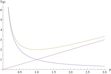
$$T_{p}(\kappa)=\dfrac{T_{1}}{p}+\kappa\dfrac{T_{1}}{2}(p-1)$$ (24)

with constant $\kappa>0$. Equation(24) has a unique minimum for $p>0$ (Fig. 3). Substituting (24) into the speedup definition 1, produces

$$S_{p}(\kappa)=\dfrac{p}{1+\kappa p(p-1)}$$ (25)

where we have absorbed the factor of 2 in $\kappa$. $S_{p}(\kappa)$ now possesses a unique maximum in the positive quadrant ($p>0$). Thus, the quadratic term in the denominator of (25) is necessary for the existence of a maximum but it is not sufficient because $S_{p}(\kappa)$ does not exhibit the Amdahl asymptote $\sigma^{-1}$ when $\kappa=0$. However, the two-parameter latency

$$T_{p}(\sigma,\kappa)=\dfrac{T_{1}}{p}+\sigma T_{1}\biggl{(}\dfrac{p-1}{p}\biggr{)}+\kappa\dfrac{T_{1}}{2}(p-1)$$ (26)

does introduce the required term into (25) and, by lemma 1, is identical to (5). ∎

Figure 3: A minimum occurs in the total latency $T(p)$ due to an increasing pairwise-exchange time being added to the initial latency reduction.

The second term in (26) can be interpreted as the fixed time it takes any one processor to broadcast a request for data and wait for the remaining fraction of processors, $(p-1)/p$, to respond simultaneously. This is also another way to view synchronous queueing in $M/M/1//p$. It simply introduces a lower bound, $\sigma T_{1}$, on the latency reduction.

The third term in (26) is analogous to Brook’s law [brooks ]: “Adding more manpower to a late software project makes it later,” with $p$ interpreted as people rather than processors. Here, for example, it can be interpreted as the latency due to the pairwise exchange of data to maintain cache coherency in a multiprocessor.

6 Conclusion

Several ubiquitous scalability models, viz., Amdahl’s law, Gustafson’s law and the universal scalability law (USL), belong to a class of rational functions. Treated as parametric models, they are neither ad hoc nor unphysical. Rather, they correspond to certain bounds on the relative throughput of the machine repairman queueing model. In the most general case, the main theorem 2 states that the USL model corresponds to the synchronous throughput bound of a load-dependent machine repairman. USL subsumes both Amdahl’s law and Gustafson’s law as corollaries of theorem 2. As well as providing a more physical basis for these scalability models, the queue-theoretic interpretation has practical significance in that it facilitates prediction of response time scalability using (7) and provides deeper insight into potential performance tuning opportunities.

Appendices

Appendix A Why Universal?

The term “universal” is intended to convey the notion that the USL (defined in Sect. 2.3) can be applied to any computer architecture; from multi-core to multi-tier. This follows from the fact that there is nothing in (5) that explicitly represents any particular system architecture or interconnect topology. That information is present but it is encoded in the numeric value of the parameters $\sigma$ and $\kappa$. The same could be said for Amdahl’s law but the difference is that, being a rational function with linear $Q(p)$, Amdahl’s law cannot predict the retrograde scalability commonly observed in performance evaluation measurements [cmg93 , gcap ]. As proven in Sect. 5, the USL is both necessary and sufficient to model all these effects.

The USL does not exclude defining a more general or more complex scalability model to account for such details as, heterogeneous processors or the functional form of degradation beyond $p^{*}$, but any such model must include the USL as a limiting case. The best analogy might be to regard the USL as being akin to Newton’s universal law of gravitation. Here, “universal” means generally applicable to any gravitating bodies. Newton’s theory has been superseded by a more sophisticated theory of gravitation; Einstein’s general theory of relativity. Einstein’s theory, however, does not negate Newton’s theory but rather, contains it as a limiting case, when space-time is flat. Since space-time is flat in all practical applications, NASA uses Newton’s equations to calculate the flight paths of all its missions.

Appendix B Synchronous Queueing

The proofs of theorem 2 (USL) and corollary 1 (Amdahl) employ mean value equations for metrics which characterize steady state conditions. As noted in remark 1, synchronized queueing cannot be maintained in steady state. Synchronization and steady state are not compatible concepts because the former is an instantaneous effect, whereas the analytic solutions we seek are only valid in long-run equilibrium.

Elsewhere [gcap , zone ], we have shown that a necessary requirement for maintaining synchronous queueing is to introduce another buffer in addition to the waiting line ($W_{1}$) at the repairman. If the extra buffer represents a post-repair collection point, such that each repaired machine (completed request) is held “off-line” until all $p$ machines are repaired then, synchronous queueing is maintained provided the $Z$ periods are i.i.d. deterministic. The extra buffer acts as a barrier synchronizer. Unfortunately, this is a $D/M/1//p$  queue, whereas the proof of corollary 1 is based on $M/M/1//p$. Moreover, the repairman performance metrics are robust [bunday ], so our results should also hold for $G/M/1//p$.

In more recent simulation experiments [zone ], we have shown that this restriction on $Z$ periods can be lifted by positioning the buffer as a pre-repair waiting room. Instead of requiring all $p$ machines to break down and enqueue simultaneously, we allow any number, less than $p$, to fail but with the added constraint that when any machine invokes service at the repairman, all other machines (or executing processors) must suspend operations as well, i.e., visit the suspension buffer. Under these conditions, $Z$ can be $G$-distributed. Because this intermittent synchronization occurs with much higher frequency and for much shorter average time periods than barrier synchronization, the potential impact of the $G$-distributed tails on the $Z$ periods is truncated.

Synchronization can be treated as a two-state Markov process, e.g., $A$: parallel and $B$: serial, where the $B$ state includes those processes that are suspended as well as waiting for service. If $\lambda_{A}$ is the transition rate for $A\to B$ and $\lambda_{B}$ for $B\to A$, then the probability of being in state $B$ is given by

$$\Pr(B)=\frac{\lambda_{B}}{\lambda_{A}+\lambda_{B}}$$ (27)

In the previous scenario it only takes a single machine to fail to suspended all other machines. The failure rate is therefore $\lambda_{A}=1/Z$ and the service rate is $\lambda_{B}=1/S$. Substituting these into (27) produces and expression identical to the serial fraction $\sigma$ in (10). In state $B$, some fraction $p_{1}$ are enqueued and the remainder $p_{2}=p-p_{1}$ are suspended. On average, any machine can expect to spend time $R=(p_{1}+p_{2})S$ to complete repairs. Hence, the total serial time is $R=pS$, which is the quantity that appears in the proofs.

Appendix C Queueing Models of Amdahl’s Law

Others have also considered Amdahl’s law from a queue-theoretic standpoint [See, e.g., kleinrock92 , nelson ]. Of these, [nelson ] is closest to our discussion, so we briefly summarize the differences.

First, the motivations are quite different. The author of [nelson ], like many other authors, seeks clever ways to defeat Amdahl’s law; in the sense of Gustafson (Sect. 2.2), whereas we are trying to understand Amdahl’s law by providing it with a more fundamental physical interpretation. Ironically, both investigations invoke queue-theoretic models to gain more insight into the pertinent issues; an open ($M/M/m$) queue in [nelson ], a closed queue (Fig. 2) in this paper.

Second, two steps are undertaken to define an alternative speedup function:

1. An attempt to unify both the Amdahl and Gustafson equations into a single speedup function.

2. Extend that unified speedup function to include waiting times.

The overarching goal is to find waiting-time optima for this unified speedup function. The unification step is achieved by purely algebraic manipulations and does not rest on any queue-theoretic arguments. The open queueing model provides an ad hoc means for incorporating waiting times as a function of queue length. The subsequent analysis is based entirely on simulation results and thereafter departs significantly from the analytic approach of this paper.

By virtue of our approach, we have shown that both Amdahl and Gustafson scaling laws are unified by the same queueing model, viz., the machine-repairman model. Moreover, corollary 1 is a lower bound on throughput; synchronous throughput, and therefore represents worst-case scalability. With this physical interpretation, it follows immediately that Amdahl’s law can be “defeated” more conveniently than proposed in [nelson ] by simply requiring that all requests be issued asynchronously [zone ].

Appendix D Remarks on the Proof of Conjecture 1

The proof in Section 5, is simplified by using the additive properties of the latency function $T_{p}$ rather than inverting the rational function $f(p)=R(p)/Q(p)$ directly. Since $Q(p)$ is quadratic in $p$, the temptation is to consider the inverse of $f^{-1}$ and use the fact that a general quadratic function has a minimum.

To see why this approach runs into difficulties, consider the simplified representation of (5):

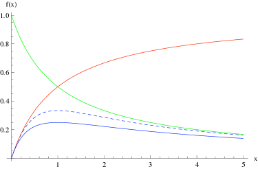
$$f(p)=\dfrac{p}{1+p+p^{2}}$$ (28)

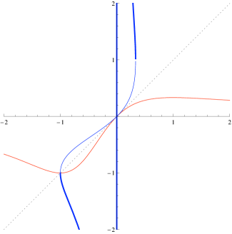
with all unit coefficients. Equation (28) is not invertible in the formal sense because $f^{-1}$ is not a one-to-one mapping, even in the positive quadrant. We can, however, consider the full inverse with its branches, as shown in Fig. 4. The principal branch is shown in light blue with the other branches occurring at the extrema of $f^{-1}$. This corresponds to the extrema of (28) occurring at $p=\pm 1\Rightarrow f(1)=\pm 1/3$. Hence, $f^{-1}\in\mathbb{C}$, $\forall p>1/3$.

Figure 4: The complete rational function (28) (red) and its inverse (blue).

Alternatively, choosing the denominator be a perfect square:

$$\dfrac{p}{1+2p+p^{2}}$$ (29)

(29) can be expressed either as a product of linear factors:

$$\dfrac{p}{1+2p+p^{2}}=\biggl{(}\dfrac{p}{1+p}\biggr{)}\biggl{(}\dfrac{1}{1+p}\biggr{)}$$

or a partial fraction expansion:

$$\dfrac{p}{1+2p+p^{2}}=\dfrac{1}{1+p}-\dfrac{1}{(1+p)^{2}}$$

Figure 5: Amdahl scaling (red), envelope function $(1+p)^{-1}$ (green), their convolution (solid blue) and equation (28) (dashed blue). The small difference in the latter two curves arises from the factor of 2 in the denominator of equation (29).

Although such decompositions are suggestive of the need for two parameters (Fig. 5), they would seem to obscure the proof of Theorem 1 rather than illuminate it. Using the latency function $T_{p}$ and then “inverting” it to produce the corresponding throughput scaling using lemma 1, avoids these problems.

Appendix E Acknowledgments

I thank Wen Chen for finding several typos in the original manuscript.

References

- [1] Wikipedia. Rational function. en.wikipedia.org/wiki/Rational_function, April 2008.
- [2] G. Amdahl. Validity of the single processor approach to achieving large scale computing capabilities. Proc. AFIPS Conf., 30:483–485, Apr. 18-20 1967.
- [3] J. L. Gustafson. “Reevaluating Amdahl’s law”. Comm. ACM, 31(5):532–533, 1988.
- [4] N. J. Gunther. “A simple capacity model for massively parallel transaction systems”. In Proc. CMG Conf., pages 1035–1044, San Diego, California, December 1993.
- [5] F. P. Preparata. Should Amdahl’s law be repealed? In ISAAC ’95: Proceedings of the 6th International Symposium on Algorithms and Computation, page 311, London, UK, Dec 4-6 1995. Springer-Verlag.
- [6] N. J. Gunther. A new interpretation of Amdahl’s law and Geometric scalability. arxiv.org/abs/cs/0210017, Oct 2002.
- [7] L. Kleinrock and J-H. Huang. On parallel processing systems: Amdahl’s law generalized and some results on optimal design. IEEE Trans. Software Eng., 18(5):434–447, 1992.
- [8] R. D. Nelson. Including queueing effects in Amdahl’s law. Comm. ACM, 39(12es):231–238, 1996.
- [9] N. J. Gunther. “Path integral methods for computer performance analysis”. Information Processing Letters, 32(1):7–13, 1989.
- [10] N. J. Gunther. Guerrilla Capacity Planning. Springer-Verlag, Heidelberg, Germany, 2007.
- [11] N. J. Gunther. Unification of Amdahl’s law, LogP and other performance models for message-passing architectures. In PDCS 2005, International Conference on Parallel and Distributed Computing Systems, pages 569–576, November 14–16, 2005, Phoenix, AZ, 2005.
- [12] J. Holtman and N. J. Gunther. Getting in the zone for successful scalability. In Proc. CMG Conf., page To appear, Las Vegas, NV, 7–12 December 2008.
- [13] W. Ware. The ultimate computer. IEEE Spectrum, 9:89–91, March 1972.
- [14] H. Sutter. Break Amdahl’s law! www.ddj.com/hpc-high-performance-computing/205900309, Jan 2008.
- [15] D. Gross and C. Harris. Fundamentals of Queueing Theory. Wiley, 1998.
- [16] D. A. Reed and R. M. Fujimoto. Multicomputer Networks: Message Based Parallel Processing. MIT Press, Boston, Mass., 1987.
- [17] M. Ajmone-Marsan, G. Balbo, and G. Conte. Performance Models of Multiprocessor Systems. MIT Press, Boston, Mass., 1990.
- [18] R. R. Muntz and J. W. Wong. Asymptotic properties of closed queueing network models. In Proc. Ann. Princeton Conf. on Inf. Sci. and Sys., pages 348–352, 1974.
- [19] J. C. S. Lui and R. R. Muntz. Computing bounds on steady state availability of repairable computer systems. Journal of the ACM, 41(4):676–707, 1994.
- [20] J. Zahorjan, K. C. Sevcik, D. L. Eager, and B. Galler. Balanced job bound analysis of queueing networks. Comm. ACM, 25(2):134–141, Feb 1982.
- [21] F. P. Brooks. The Mythical Man-Month. Addison-Wesley, Reading, MA, anniversary edition, 1995.
- [22] B. D. Bunday and R. E. Scraton. The machine interference model. European Journal of Operations Research, 4:399–402, 1980.