Large-scale magnetic topologies of mid-M dwarfs

Abstract

We present in this paper the first results of a spectropolarimetric analysis of a small sample ($\sim 20$) of active stars ranging from spectral type M0 to M8, which are either fully-convective or possess a very small radiative core. This study aims at providing new constraints on dynamo processes in fully-convective stars.

The present paper focuses on 5 stars of spectral type $\sim$M4, i.e. with masses close to the full convection threshold ($\simeq 0.35~{}\hbox{${\rm M}_{\odot}$}$), and with short rotational periods. Tomographic imaging techniques allow us to reconstruct the surface magnetic topologies from the rotationally modulated time-series of circularly polarised profiles. We find that all stars host mainly axisymmetric large-scale poloidal fields. Three stars were observed at two different epochs separated by $\sim$1 yr; we find the magnetic topologies to be globally stable on this timescale.

We also provide an accurate estimation of the rotational period of all stars, thus allowing us to start studying how rotation impacts the large-scale magnetic field.

1 Introduction

Magnetic fields play a key role in every phase of the life of stars and are linked to most of their manifestations of activity. Since Larmor (1919) first proposed that electromagnetic induction might be the origin of the Sun’s magnetic field, dynamo generation of magnetic fields in the Sun and other cool stars has been a subject of constant interest. The paradigm of the $\alpha\Omega$ dynamo, i.e. the generation of a large-scale magnetic field through the combined action of differential rotation ($\Omega$ effect) and cyclonic convection ($\alpha$ effect), was first proposed by Parker (1955) and then thoroughly debated and improved (e.g., Babcock, 1961; Leighton, 1969). A decade ago, helioseismology provided the first measurements of the internal differential rotation in the Sun and thus revealed a thin zone of strong shear at the interface between the radiative core and the convective envelope. During the past few years, theoreticians pointed out the crucial role for dynamo processes of this interface – called the tachocline – being the place where the $\Omega$ effect can amplify magnetic fields (see Charbonneau 2005 for a review of solar dynamo models).

Among cool stars, those with masses lower than about 0.35 ${\rm M}_{\odot}$ are fully-convective (e.g., Chabrier & Baraffe, 1997), and therefore do not possess a tachocline; some observations further suggest that they rotate almost as rigid bodies (Barnes et al., 2005). However, many fully-convective stars are known to show various signs of activity such as radio, Balmer line, and X-ray emissions (e.g., Joy & Humason, 1949; Lovell et al., 1963; Delfosse et al., 1998; Mohanty & Basri, 2003; West et al., 2004). Magnetic fields have been directly detected thanks to Zeeman effect on spectral lines, either in unpolarised light (e.g., Saar & Linsky, 1985; Johns-Krull & Valenti, 1996; Reiners & Basri, 2006), or in circularly polarised spectra (Donati et al., 2006).

The lack of a tachocline in very-low-mass stars led theoreticians to propose non-solar dynamo mechanism in which cyclonic convection and turbulence play the main roles while differential rotation only has minor effects (e.g., Durney et al., 1993). During past few years, several semi-analytical approaches and MHD simulations were developed in order to model the generation of magnetic fields in fully-convective stars. Although they all conclude that fully-convective stars should be able to produce a large-scale magnetic field, they disagree on the properties of such a field, and the precise mechanisms involved in the dynamo effect remain unclear. Mean-field modellings by Küker & Rüdiger (2005) and Chabrier & Küker (2006) assumed solid-body rotation and found $\alpha^{2}$ dynamo generating purely non-axisymmetric large-scale fields. Subsequent direct numerical simulations diagnose either “antisolar” differential rotation (i.e. poles faster than the equator) associated with a net axisymmetric poloidal field (e.g., Dobler et al., 2006); or strongly quenched “solar” differential rotation (i.e. the equator faster than the poles) and a strong axisymmetric toroidal field component (e.g., Browning, 2008).

The first detailed observations of fully-convective stars do not completely agree with any of these models. Among low-mass stars, differential rotation appears to vanish with increasing convective depth (Barnes et al., 2005). This result is further confirmed by the first detailed spectropolarimetric observations of the very active fully-convective star V374 Peg by Donati et al. (2006) and Morin et al. (2008) (hereafter M08) who measure very weak differential rotation (about 1/10th of the solar surface shear). These studies also report a strong mostly axisymmetric poloidal surface magnetic field stable on a timescale of 1 yr on V374 Peg, a result which does not completely agree with any of the existing theoretical predictions. V374 Peg being a very fast rotator, observations of fully-convective stars with longer rotation periods are necessary to generalise these results.

In order to provide theoretical models and numerical simulations with better constraints, it is necessary to determine the main magnetic field properties – topology and time-variability – of several fully-convective stars, and to find out their dependency on stellar parameters – mass, rotation rate, and differential rotation. In this paper, we present and analyse the spectropolarimetric observations of a small sample of stars just around the limit to full convection (spectral types ranging from M3 to M4.5), collected with ESPaDOnS and NARVAL between 2006 Jan and 2008 Feb. Firstly, we briefly present our stellar sample, and our observations are described in a second part. We then provide insight on the imaging process and associated physical model. Afterwards, we present our analysis for each star of the sample. Finally, we discuss the global trends found in our sample and their implications in the understanding of dynamo processes in fully-convective stars.

2 Stellar sample

Our stellar sample includes 5 M-dwarfs just about the full-convection threshold i.e. around spectral type M4. It is part of a wider sample of about 20 stars ranging from M0 to M8; results for remaining stars will be presented in forthcoming papers. The stars were selected from the rotation-activity study of Delfosse et al. (1998). We chose only active stars so that the magnetic field is strong enough to produce detectable circularly polarised signatures, allowing us to apply tomographic imaging techniques. Stars with spin periods ranging from 0.4 to 4.4 $\rm d$ were selected to study the impact of rotation on the reconstructed magnetic topologies (though all the observed stars lie in the saturated regime, see Sec. 10).

Table 1: Fundamental parameters of the stellar sample. Columns 1–8 respectively list the name, the spectral type (taken from Reid et al., 1995), the stellar mass (see Sec. 2), the bolometric luminosity and log$R_{X}=$log($L_{X}/L_{bol}$) (see text), the projected rotation velocity as inferred from Zeeman Doppler Imaging (ZDI), and the rotation periods $P_{ZDI}$ (used to compute the ephemeris) and $P_{\rm rot}$ (accurate period derived from our study). Columns 9–13 respectively list the empirical convective turnover time (see text), the effective Rossby number (see text), the $R\sin i$ , the theoretical radius suited to the stellar mass (see text), and the inclination angle used for ZDI deduced by comparing columns 11 and 12. For columns 8 and 11 we also mention, between brackets, respectively 3-$\sigma$ and 1-$\sigma$ error bars inferred from our study. For the precision of the other quantities refer to Section 2.

Name	ST	$M_{\star}$	log$L_{bol}$	log$R_{X}$	$v\sin i$	$P_{\rm ZDI}$	$P_{\rm rot}$	$\tau_{c}$	$Ro$	$R\sin i$	$R_{\star}$	$i$
		(${\rm M}_{\odot}$)	(erg s-1)		(km s-1)	(d)	(d)	(d)	($10^{-2}$)	(${\rm R}_{\odot}$)	(${\rm R}_{\odot}$)	(∘)
AD Leo	M3	$0.42$	31.91	-3.18	$3.0$	2.22	$2.2399(6)$	48	4.7	$0.13(4)$	0.38	20
EQ Peg A	M3.5	$0.39$	31.84	-3.02	$17.5$	$1.06$	$1.061(4)$	54	2.0	$0.37(2)$	0.35	60
EV Lac	M3.5	$0.32$	31.66	-3.33	$4.0$	4.378	$4.3715(6)$	64	6.8	$0.35(9)$	0.30	60
YZ CMi	M4.5	$0.31$	31.64	-3.09	$5.0$	2.77	$2.7758(6)$	66	4.2	$0.27(5)$	0.29	60
V374 Peg	M4	$0.28$	31.56	-3.20	$36.5$	–	$0.445654(2)$	72	0.6	$0.32(1)$	0.28	70
EQ Peg B	M4.5	$0.25$	31.47	-3.25	$28.5$	0.405	$0.404(4)$	76	0.5	$0.23(1)$	0.25	60

The analysis carried out in the present paper concerns: AD Leo (GJ 388) which is partly-convective, EV Lac (GJ 873), YZ  CMi (GJ 285), EQ Peg A (GJ 896 A) which lies just on the theoretical limit to full-convection, and EQ Peg B (GJ 896 B). All are known as active flare-stars, and strong magnetic fields have already been reported for some stars (e.g., Saar & Linsky, 1985; Johns-Krull & Valenti, 1996; Reiners & Basri, 2007). We include the previously studied M4 star V374 Peg in our analysis (M08).

The main properties of the stellar sample, inferred from the present work or collected from previous ones, are shown in Table 1. We show stellar masses computed using the empirical relation derived by Delfosse et al. (2000) and based on J-band absolute magnitude values inferred from apparent magnitude measurements of 2MASS (Cutri et al., 2003) and Hipparcos parallaxes (ESA, 1997). For EQ Peg A and B, the values we find are in good agreement with the dynamical mass of the binary system of $0.61\pm 0.03$ reported by Tamazian et al. (2006). Radius and bolometric luminosity suited to the stellar mass are computed from NextGen models (Baraffe et al., 1998). We also mention log$R_{X}=$ log($L_{X}/L_{bol}$), where $L_{X}$ is an average of NEXXUS values (excluding outliers supposedly corresponding to flares). We observe dispersions ranging from 0.1 to 0.2 in log($L_{X}$), corresponding to intrinsic variability. As no data is available on NEXXUS for EQ Peg B alone, we take one fourth of EQ Peg A’s X-ray luminosity, as reported by Robrade et al. (2004). Line of sight projected equatorial velocities ($v\sin i$), rotation periods ($P_{\rm rot}$) and inclination ($i$) of the rotation axis with respect to the line of sight are inferred from the present study. We estimate that the absolute accuracy to which $v\sin i$ is determined is about 1 km s^-1. The uncertainty on $P_{\rm rot}$ is precisely computed (see 4.3). The inclination angle estimate is coarse (accuracy of about 20^∘), tomographic imaging does not require more precision.

To study how activity and magnetic fields vary among stars of different masses, the most relevant parameter to consider is the effective Rossby number $Ro=\hbox{$P_{\rm rot}$}/\tau_{c}$ (where $\tau_{c}$ is the convective turnover time, Noyes et al. 1984, e.g.,). We take convective turnover times from Kiraga & Stepien (2007, empirically derived from X ray fluxes of M dwarfs); $\tau_{c}$ is found to increase strongly (as expected) with decreasing mass and bolometric luminosities. For the present sample, we find that $Ro$ ranges from 0.005 to 0.07, i.e., much smaller than in the Sun (where $Ro\simeq 1.5-2.0$) as a result of both the shorter $P_{\rm rot}$ and the larger $\tau_{c}$ (see Table 1).

3 Observations

Spectropolarimetric observation of our 5 mid-M stars were collected between 2006 Jan and 2008 Feb with the twin instruments ESPaDOnS on the 3.6m Canada-France-Hawaii Telescope (CFHT) located in Hawaii, and NARVAL on the 2m Télescope Bernard Lyot (TBL) in southern France. ESPaDOnS and NARVAL are built from the same design (Donati, 2003c). They produce spectra spanning the entire optical domain (from 370 to 1000 nm) at a resolving power of about 65 000. Each observation consists of four individual subexposures taken in different polarimeter configurations which are combined together so that all spurious polarisation signatures are cancelled to first order (e.g., Donati et al., 1997a).

Data reduction was carried out using libre-esprit. This fully automated package/pipeline installed at CFHT and TBL performs optimal extraction of NARVAL and ESPaDOnS unpolarised (Stokes $I$) and circularly polarised (Stokes $V$) spectra, following the procedure described in Donati et al. (1997a). The peak signal-to-noise ratios (S/N) per 2.6 km s^-1 velocity bin range from 100 to 500, depending on the magnitude of the target, the telescope used and the weather conditions. The full journal of observations is presented in Tables LABEL:tab:log_adleo to LABEL:tab:log_eqpegb.

All spectra are automatically corrected for spectral shifts resulting from instrumental effects (e.g., mechanical flexures, temperature or pressure variations) using telluric lines as a reference. Though not perfect, this procedure allows spectra to be secured with a radial velocity (RV) precision of better than $0.030~{}\hbox{km\,s${}^{-1}$}$ (e.g., Moutou et al., 2007).

Least-squares deconvolution (LSD, Donati et al., 1997a) was applied to all observations, in order to extract the polarimetric information from most photospheric atomic lines and gather it into a unique synthetic profile of central wavelength $\lambda_{0}=700~{}{\rm nm}$ and effective Landé factor $g_{\rm eff}=1.2$. The line list for LSD was computed from an Atlas9 local thermodynamic equilibrium model (Kurucz, 1993) matching the properties properties of our whole sample, and contains about 5 000 moderate to strong atomic lines. We notice a multiplex gain of about 10 with respect to the S/N of the individual spectra of our sample. Zeeman signatures are clearly detected in all the spectra (see Sec. 5 to 9) with maximum amplitudes varying from 0.5% (for EQ Peg B) to 1.2% (for AD Leo) of the unpolarised continuum level. Temporal variations, due to rotational modulation, of the Zeeman signatures is obvious for some stars, whereas it is very weak on others, mostly depending on the inclination angle of their rotation axis with respect to the line of sight.

For each observation we compute the corresponding longitudinal magnetic field (i.e. the line of sight projection) from the Stokes $I$ and $V$ LSD profiles through the relation :

$$B_{l}({\rm G})=-2.14\times 10^{11}\frac{\displaystyle\int v\,V(v)\,{\rm d}v}{\lambda_{0}\,g_{\rm eff}\,c\displaystyle\int\left[I_{c}-I(v)\right]{\rm d}v}\,,$$ (1)

(Rees & Semel, 1979; Donati et al., 1997a; Wade et al., 2000) where $v$ is the radial velocity in the star’s rest frame, $\lambda_{0}$, in nm, is the mean wavelength of the LSD profile, $c$ is the velocity of light in vacuum in the same unit as $v$, $g_{\rm eff}$ is the value of the mean Landé factor of the LSD line, and $I_{c}$ the continuum level.

In the rest of the paper, all data are phased according to the following ephemeris:

$$\mbox{HJD}=2453950.0+P_{ZDI}E.$$ (2)

where $P_{ZDI}$ is the rotational period used as an input for ZDI and given in Table 1.

Table 2: Journal of observations for AD Leo. Columns 1–7 list the UT date, the heliocentric Julian date, the UT time, the observation site, the exposure time, the peak signal to noise ratio (per 2.6 km s^-1 velocity bin) and the rms noise level (relative to the unpolarised continuum level and per 1.8 km s^-1 velocity bin) in the average circular polarisation profile produced by Least-Squares Deconvolution (see Sec. 3). In column 8 we indicate the longitudinal field computed from Eq. 1. The rotational cycle $E$ from the ephemeris of Eq. 2 is given in column 9. Column 10 lists the radial velocities (absolute accuracy $0.10~{}\hbox{km\,s${}^{-1}$}$, internal accuracy $0.03~{}\hbox{km\,s${}^{-1}$}$) associated to each exposure.

Date	HJD	UT	Obs. site	$t_{\rm exp}$	S/N	$\sigma_{\rm LSD}$	$B_{\ell}$	Cycle	$v_{r}$
	(2,453,000+)	(h:m:s)		(s)		($10^{-4}I_{\rm c}$)	(G)		(km s-1)
2007
Jan 27	4127.59748	02:14:28	TBL	4 $\times$ 600.0	274	2.6	-294.9 $\pm$ 12.9	79.999	12.40
Jan 28	4128.60883	02:30:45	TBL	4 $\times$ 600.0	401	1.7	-233.4 $\pm$ 8.9	80.454	12.40
Jan 29	4129.57169	01:37:14	TBL	4 $\times$ 600.0	393	1.7	-298.2 $\pm$ 10.0	80.888	12.46
Jan 30	4130.60841	02:30:03	TBL	4 $\times$ 600.0	472	1.4	-252.6 $\pm$ 8.0	81.355	12.36
Feb 01	4132.59818	02:15:14	TBL	4 $\times$ 600.0	338	2.1	-252.1 $\pm$ 10.6	82.251	12.34
Feb 02	4133.63116	03:02:41	TBL	4 $\times$ 600.0	428	1.6	-262.5 $\pm$ 8.6	82.717	12.44
Feb 03	4134.61119	02:33:53	TBL	4 $\times$ 600.0	395	1.7	-262.9 $\pm$ 9.3	83.158	12.34
Feb 04	4135.62167	02:48:56	TBL	4 $\times$ 600.0	411	1.7	-238.5 $\pm$ 8.7	83.613	12.42
Feb 05	4136.59250	02:06:53	TBL	4 $\times$ 600.0	348	2.0	-295.9 $\pm$ 10.8	84.051	12.38
2008
Jan 19	4485.51772	00:20:02	TBL	4 $\times$ 800.0	329	2.3	-275.1 $\pm$ 11.1	241.224	12.40
Jan 24	4489.56829	01:32:36	TBL	4 $\times$ 600.0	398	1.8	-245.6 $\pm$ 8.8	243.049	12.40
Jan 27	4492.53788	00:48:39	TBL	4 $\times$ 600.0	408	1.7	-284.2 $\pm$ 8.8	244.386	12.34
Jan 28	4493.54864	01:04:06	TBL	4 $\times$ 600.0	398	1.8	-219.1 $\pm$ 8.9	244.842	12.29
Jan 30	4495.56109	01:21:56	TBL	4 $\times$ 600.0	341	2.2	-208.5 $\pm$ 10.1	245.748	12.32
Feb 03	4499.56749	01:30:58	TBL	4 $\times$ 600.0	376	1.9	-259.2 $\pm$ 9.6	247.553	12.28
Feb 05	4501.54728	01:01:47	TBL	4 $\times$ 600.0	355	2.0	-288.3 $\pm$ 10.1	248.445	12.34
Feb 06	4502.54747	01:02:02	TBL	4 $\times$ 600.0	414	1.7	-204.4 $\pm$ 8.1	248.895	12.33
Feb 10	4506.55755	01:16:25	TBL	4 $\times$ 600.0	413	1.7	-224.7 $\pm$ 8.2	250.702	12.36
Feb 12	4508.55161	01:07:49	TBL	4 $\times$ 600.0	398	1.8	-257.9 $\pm$ 8.9	251.600	12.34
Feb 13	4509.55640	01:14:42	TBL	4 $\times$ 600.0	398	2.2	-234.9 $\pm$ 11.7	252.052	12.40
Feb 14	4510.55228	01:08:45	TBL	4 $\times$ 600.0	279	2.7	-281.3 $\pm$ 12.4	252.501	12.27
Feb 15	4511.56943	01:33:25	TBL	4 $\times$ 600.0	388	1.9	-196.0 $\pm$ 8.6	252.959	12.39
Feb 16	4512.55367	01:10:42	TBL	4 $\times$ 600.0	405	1.7	-283.6 $\pm$ 8.8	253.403	12.36

Table 3: Same as Table LABEL:tab:log_adleo for EV Lac.

Date	HJD	UT	Ob. site	$t_{\rm exp}$	S/N	$\sigma_{\rm LSD}$	$B_{\ell}$	Cycle	$v_{r}$
	(2,453,000+)	(h:m:s)		(s)		($10^{-4}I_{\rm c}$)	(G)		(km s-1)
2006
Aug 05	3953.07311	13:38:30	CFHT	4 $\times$ 300.0	368	2.2	-556.8 $\pm$ 17.8	0.702	0.30
Aug 07	3955.06634	13:28:36	CFHT	4 $\times$ 300.0	379	2.0	343.7 $\pm$ 13.3	1.157	0.14
Aug 08	3956.06002	13:19:26	CFHT	4 $\times$ 400.0	437	1.7	-380.1 $\pm$ 12.2	1.384	0.40
Aug 09	3957.05969	13:18:53	CFHT	4 $\times$ 230.0	334	2.3	-464.6 $\pm$ 16.3	1.613	0.35
Aug 10	3958.07230	13:36:58	CFHT	4 $\times$ 250.0	332	2.4	-355.6 $\pm$ 15.2	1.844	0.38
Aug 11	3959.07281	13:37:39	CFHT	4 $\times$ 250.0	353	2.2	297.2 $\pm$ 14.0	2.072	0.05
Aug 12	3960.07608	13:42:17	CFHT	4 $\times$ 250.0	329	2.5	-158.6 $\pm$ 14.4	2.302	0.33
2007
Jul 28	4309.54645	01:00:53	TBL	4 $\times$ 900.0	439	1.8	59.8 $\pm$ 10.5	82.126	0.30
Jul 29	4310.56610	01:29:05	TBL	4 $\times$ 900.0	399	1.8	-421.5 $\pm$ 14.7	82.359	0.49
Jul 30	4311.59374	02:08:47	TBL	4 $\times$ 900.0	360	2.0	-527.4 $\pm$ 17.3	82.593	0.60
Jul 31	4312.59372	02:08:40	TBL	4 $\times$ 600.0	326	2.5	34.2 $\pm$ 14.4	82.822	0.22
Aug 01	4313.59576	02:11:31	TBL	4 $\times$ 600.0	281	3.0	267.6 $\pm$ 18.5	83.051	0.30
Aug 03	4315.60183	02:20:05	TBL	4 $\times$ 600.0	306	2.5	-481.7 $\pm$ 18.8	83.509	0.62
Aug 04	4316.59985	02:17:09	TBL	4 $\times$ 600.0	330	2.4	-271.4 $\pm$ 15.5	83.737	0.29
Aug 05	4317.67118	03:59:47	TBL	4 $\times$ 600.0	273	3.0	338.1 $\pm$ 19.1	83.982	0.46
Aug 10	4322.59520	02:09:60	TBL	4 $\times$ 600.0	303	2.7	107.0 $\pm$ 16.1	85.106	0.26
Aug 11	4323.59772	02:13:34	TBL	4 $\times$ 600.0	235	3.5	-353.7 $\pm$ 21.1	85.335	0.47
Aug 15	4327.58824	01:59:40	TBL	4 $\times$ 600.0	301	2.5	-318.8 $\pm$ 16.8	86.247	0.30
Aug 18	4330.58129	01:49:29	TBL	4 $\times$ 600.0	308	2.4	378.2 $\pm$ 17.0	86.930	0.29
Aug 19	4331.51487	00:13:47	TBL	4 $\times$ 600.0	339	2.3	-62.2 $\pm$ 13.8	87.144	0.21
Aug 28	4340.53002	00:35:14	TBL	4 $\times$ 600.0	279	2.8	-235.8 $\pm$ 17.8	89.203	0.30
Aug 31	4343.52117	00:22:25	TBL	4 $\times$ 600.0	258	3.1	232.7 $\pm$ 18.6	89.886	0.30

Table 4: Same as Table LABEL:tab:log_adleo for YZ CMi.

Date	HJD	UT	Ob. site	$t_{\rm exp}$	S/N	$\sigma_{\rm LSD}$	$B_{\ell}$	Cycle	$v_{r}$
	(2,453,000+)	(h:m:s)		(s)		($10^{-4}I_{\rm c}$)	(G)		(km s-1)
2007
Jan 26	4127.43869	22:24:17	TBL	4 $\times$ 900.0	235	3.9	-401.9 $\pm$ 31.4	64.057	26.66
Jan 27	4128.47944	23:22:59	TBL	4 $\times$ 900.0	255	3.3	-782.5 $\pm$ 33.3	64.433	26.60
Jan 29	4130.47395	23:15:08	TBL	4 $\times$ 900.0	324	2.6	-520.4 $\pm$ 25.3	65.153	26.74
Feb 01	4133.50014	23:52:56	TBL	4 $\times$ 900.0	254	3.7	-710.2 $\pm$ 40.3	66.246	26.82
Feb 03	4135.49442	23:44:47	TBL	4 $\times$ 900.0	280	3.3	-156.7 $\pm$ 25.1	66.965	26.51
Feb 04	4136.46196	22:58:05	TBL	4 $\times$ 900.0	261	3.4	-781.5 $\pm$ 36.3	67.315	26.66
Feb 08	4140.47749	23:20:37	TBL	4 $\times$ 900.0	260	3.8	-62.3 $\pm$ 27.9	68.764	26.44
Dec 28	4462.62633	02:54:53	TBL	4 $\times$ 1200.0	289	3.9	-279.8 $\pm$ 28.6	185.064	26.28
Dec 29	4463.65629	03:37:59	TBL	4 $\times$ 1200.0	323	3.0	-560.9 $\pm$ 27.0	185.435	26.75
Dec 31	4465.67053	03:58:24	TBL	4 $\times$ 900.0	238	4.4	-166.5 $\pm$ 30.2	186.163	26.43
2008
Jan 01	4466.66384	03:48:43	TBL	4 $\times$ 1100.0	305	3.0	-680.3 $\pm$ 29.4	186.521	26.59
Jan 03	4468.66111	03:44:43	TBL	4 $\times$ 1100.0	272	3.7	-97.7 $\pm$ 26.3	187.242	26.69
Jan 20	4485.93731	10:22:12	CFHT	4 $\times$ 220.0	240	3.9	-599.6 $\pm$ 31.0	193.479	26.65
Jan 23	4488.52001	00:21:18	TBL	4 $\times$ 1200.0	281	3.3	-452.3 $\pm$ 26.7	194.412	26.76
Jan 23	4489.45108	22:42:04	TBL	4 $\times$ 1200.0	252	3.8	-624.4 $\pm$ 32.0	194.748	26.84
Jan 24	4490.53391	00:41:21	TBL	4 $\times$ 1200.0	290	3.4	-258.2 $\pm$ 24.8	195.139	26.34
Jan 25	4491.46536	23:02:40	TBL	4 $\times$ 1200.0	254	3.9	-575.7 $\pm$ 31.2	195.475	26.68
Jan 26	4492.45361	22:45:46	TBL	4 $\times$ 1200.0	317	3.1	-538.7 $\pm$ 27.4	195.832	26.82
Jan 27	4493.46567	23:03:09	TBL	4 $\times$ 1200.0	324	3.2	-116.5 $\pm$ 22.8	196.197	26.46
Jan 28	4494.53067	00:36:46	TBL	4 $\times$ 1200.0	260	3.8	-724.1 $\pm$ 35.0	196.581	26.57
Jan 29	4495.47886	23:22:12	TBL	4 $\times$ 1200.0	294	3.6	-537.6 $\pm$ 32.6	196.924	26.37
Feb 02	4499.47856	23:21:54	TBL	4 $\times$ 1200.0	281	3.7	-292.8 $\pm$ 26.5	198.368	26.74
Feb 04	4501.45937	22:54:20	TBL	4 $\times$ 1200.0	217	5.0	-410.1 $\pm$ 36.2	199.083	26.15
Feb 05	4502.46143	22:57:21	TBL	4 $\times$ 1200.0	299	3.4	-456.3 $\pm$ 28.4	199.445	26.66
Feb 06	4503.49639	23:47:44	TBL	4 $\times$ 1200.0	316	3.1	-533.7 $\pm$ 26.6	199.818	26.80
Feb 09	4506.46767	23:06:31	TBL	4 $\times$ 1200.0	124	8.4	-491.3 $\pm$ 58.9	200.891	26.71
Feb 11	4508.46975	23:09:38	TBL	4 $\times$ 1200.0	282	3.2	-686.2 $\pm$ 29.7	201.614	26.60
Feb 12	4509.47423	23:16:08	TBL	4 $\times$ 1200.0	317	3.2	-485.5 $\pm$ 26.4	201.976	26.49
Feb 13	4510.46991	23:09:58	TBL	4 $\times$ 1200.0	268	3.7	-165.3 $\pm$ 25.5	202.336	26.76
Feb 14	4511.48644	23:33:50	TBL	4 $\times$ 1200.0	280	3.5	-653.1 $\pm$ 30.6	202.703	26.74
Feb 15	4512.47158	23:12:30	TBL	4 $\times$ 1200.0	320	3.2	-421.7 $\pm$ 25.6	203.058	26.17
Feb 16	4513.47114	23:11:56	TBL	4 $\times$ 1200.0	326	3.0	-351.3 $\pm$ 23.6	203.419	26.79

Table 5: Same as Table LABEL:tab:log_adleo for EQ Peg A.

Date	HJD	UT	Ob. site	$t_{\rm exp}$	S/N	$\sigma_{\rm LSD}$	$B_{\ell}$	Cycle	$v_{r}$
	(2,453,000+)	(h:m:s)		(s)		($10^{-4}I_{\rm c}$)	(G)		(km s-1)
2006
Aug 05	3952.99538	11:46:33	CFHT	4 $\times$ 200.0	322	2.5	264.9 $\pm$ 18.6	2.799	0.39
Aug 05	3953.11181	14:34:13	CFHT	4 $\times$ 160.0	295	2.9	191.0 $\pm$ 20.4	2.908	0.78
Aug 07	3954.97268	11:13:40	CFHT	4 $\times$ 200.0	327	2.5	409.9 $\pm$ 19.4	4.647	0.27
Aug 07	3955.13847	15:12:24	CFHT	4 $\times$ 200.0	323	2.6	279.0 $\pm$ 18.8	4.802	0.47
Aug 08	3955.98480	11:31:02	CFHT	4 $\times$ 160.0	283	3.0	412.4 $\pm$ 22.3	5.593	0.31
Aug 08	3956.14334	15:19:20	CFHT	4 $\times$ 300.0	374	2.1	326.9 $\pm$ 16.2	5.741	0.34
Aug 09	3956.99077	11:39:32	CFHT	4 $\times$ 160.0	261	3.2	427.8 $\pm$ 23.6	6.533	0.28
Aug 09	3957.12529	14:53:14	CFHT	4 $\times$ 160.0	289	2.9	412.4 $\pm$ 21.7	6.659	0.31
Aug 09	3957.13682	15:09:50	CFHT	4 $\times$ 160.0	284	2.9	409.9 $\pm$ 21.8	6.670	0.30
Aug 10	3957.98897	11:36:51	CFHT	4 $\times$ 160.0	296	2.9	427.8 $\pm$ 21.9	7.466	0.21
Aug 10	3958.14147	15:16:26	CFHT	4 $\times$ 160.0	273	3.1	460.5 $\pm$ 23.1	7.609	0.34
Aug 11	3958.99132	11:40:09	CFHT	4 $\times$ 160.0	290	3.1	379.4 $\pm$ 22.3	8.403	0.10
Aug 11	3959.13871	15:12:23	CFHT	4 $\times$ 160.0	274	3.1	433.1 $\pm$ 23.1	8.541	0.32
Aug 12	3959.99595	11:46:44	CFHT	4 $\times$ 160.0	272	3.4	379.3 $\pm$ 24.3	9.342	-0.04
Aug 12	3960.14401	15:19:55	CFHT	4 $\times$ 160.0	262	3.5	382.2 $\pm$ 24.8	9.480	0.25

Table 6: Same as Table LABEL:tab:log_adleo for EQ Peg B.

Date	HJD	UT	Ob. site	$t_{\rm exp}$	S/N	$\sigma_{\rm LSD}$	$B_{\ell}$	Cycle	$v_{r}$
	(2,453,000+)	(h:m:s)		(s)		($10^{-4}I_{\rm c}$)	(G)		(km s-1)
Aug 05	3953.01352	12:12:41	CFHT	4 $\times$ 320.0	194	5.5	315.4 $\pm$ 40.8	4.532	3.32
Aug 05	3953.09585	14:11:14	CFHT	4 $\times$ 320.0	194	5.4	403.9 $\pm$ 41.4	4.655	3.32
Aug 07	3955.00502	12:00:15	CFHT	4 $\times$ 320.0	194	5.5	296.5 $\pm$ 40.5	7.526	3.31
Aug 07	3955.12027	14:46:12	CFHT	4 $\times$ 320.0	187	5.6	358.5 $\pm$ 41.5	7.700	3.41
Aug 08	3956.00013	11:53:06	CFHT	4 $\times$ 300.0	187	5.8	243.4 $\pm$ 42.3	9.023	3.48
Aug 08	3956.12205	14:48:40	CFHT	4 $\times$ 400.0	222	4.7	197.8 $\pm$ 35.7	9.206	3.10
Aug 09	3957.00746	12:03:34	CFHT	4 $\times$ 280.0	178	6.0	278.2 $\pm$ 44.1	10.538	3.45
Aug 09	3957.10933	14:30:16	CFHT	4 $\times$ 280.0	180	6.0	376.4 $\pm$ 44.5	10.691	3.26
Aug 10	3958.00771	12:03:51	CFHT	4 $\times$ 300.0	176	6.1	204.8 $\pm$ 44.0	12.042	3.51
Aug 10	3958.12127	14:47:22	CFHT	4 $\times$ 300.0	178	6.0	205.1 $\pm$ 43.5	12.212	3.16
Aug 11	3959.00904	12:05:40	CFHT	4 $\times$ 300.0	150	7.4	287.3 $\pm$ 52.7	13.547	3.38
Aug 12	3960.01246	12:10:30	CFHT	4 $\times$ 300.0	152	7.2	222.1 $\pm$ 50.4	15.056	3.62
Aug 12	3960.12839	14:57:26	CFHT	4 $\times$ 300.0	155	7.4	299.5 $\pm$ 51.0	15.231	3.08

4 Model description

For each star of our sample, our aim is to infer the topology of the surface magnetic field from the time series of circularly polarised (Stokes $V$) LSD profiles we obtained. This can be achieved using a tomographic imaging code. In this part we briefly present the main features of our imaging code, the physical model used to describe the Stokes $I$ and $V$ line profiles, and the way we use this code to provide constraints on rotational period and differential rotation.

4.1 Zeeman-Doppler Imaging (ZDI)

Circularly polarised light emitted by a star informs us about the longitudinal magnetic field at its surface. Thanks to the Doppler effect, magnetic regions at the surface of a rapidly rotating star produce Stokes $V$ signatures whose wavelength strongly correlates with their spatial position; in this respect a circularly polarised line profile can be seen as 1D image of the longitudinal magnetic field. By analysing how these signatures are modulated by rotation, it is possible to reconstruct a 2D map of the surface magnetic field. See Brown et al. (1991) and Donati & Brown (1997b) for more details about ZDI and its performances. As we demonstrate in this paper, and was already shown by Donati et al. (2006) for $\tau$ Sco ($\hbox{$v\sin i$}\simeq 5~{}\hbox{km\,s${}^{-1}$}$), even for slowly rotating stars ZDI is able to recover some information about the large-scale surface magnetic field. In all cases, we need to set $\ell>6$ to be able to reproduce rotational modulation in our data.

The ZDI code we employ here is based on a spherical harmonics description of each component of the magnetic field vector, implemented by Donati et al. (2006). Compared with the conventional ZDI technique (which described the field as a set of independent values), this approach allows us to reconstruct a physically meaningful magnetic field as the sum of a poloidal field and a toroidal field (Chandrasekhar, 1961). Such a decomposition is of obvious interest for all studies on stellar dynamos. Moreover, this method proved to be more efficient than the old one at recovering simple low order topologies such as dipoles, even from Stokes $V$ data sets only (Donati et al., 2001).

ZDI works by comparing observational data to synthetic spectra computed from a guess magnetic map. The map is iteratively updated until the corresponding spectra fit the observations within a given $\chi^{2}$ level. In order to compute the synthetic spectra, the surface of the star is divided into a grid of $\sim 1,000$ cells on which the magnetic field components are computed from the coefficients of the spherical harmonics expansion. The contribution of each individual pixel is computed from a model based on Unno-Rachkovsky’s equations (see Sec. 4.2).

Given the projected rotational velocities for our sample ($\hbox{$v\sin i$}<30~{}\hbox{km\,s${}^{-1}$}$) and considering the local profile width ($\simeq 9~{}\hbox{km\,s${}^{-1}$}$, M08), we infer that the maximum number of spatially resolved elements across the equator is about 20. Therefore, using a grid of 1,000 cells at the surface of the star (the equatorial ring of the grid is made of about 70 elements, depending on the inclination of the star) is perfectly adequate for our needs.

As the inversion problem is partly ill-posed, several magnetic topologies can fit a set of observations, for a given $\chi^{2}$ level. Optimal reconstruction is achieved by choosing the maximum entropy solution, i.e. the one which contains the least informational content (Skilling & Bryan, 1984). We chose here a quadratic form for the entropy :

$$S=-\sum_{\ell,m}\ell\left(\alpha_{\ell,m}^{2}+\beta_{\ell,m}^{2}+\gamma_{\ell,m}^{2}\right)$$ (3)

where $\alpha_{\ell,m}$, $\beta_{\ell,m}$, $\gamma_{\ell,m}$ are the spherical harmonics coefficient of order $(\ell,m)$ describing respectively the radial, orthoradial poloidal and toroidal field components (see Donati et al., 2006, for more details). This functional, one of the simplest possible forms, is well-suited for magnetic fields reconstruction since it allows for negative values (as opposed to the conventional expression of the Shannon entropy).

4.2 Modelling of the local line profiles

As explained in Sec. 4.1, the local Stokes $I$ and $V$ line profiles are computed from a simple model based on Unno-Rachkovsky’s equations (Unno, 1956), similar to that used by Donati et al. (2008). We add two degrees of freedom to the Unno-Rachkovsky’s model, the filling factors $f_{I}$ and $f_{V}$:

$$\left\{\begin{array}[]{l}I=f_{I}\times\hbox{$I_{\rm UR}$}(\lambda_{B})+(1-f_{I})\times\hbox{$I_{\rm q}$}\\ V=f_{V}\times\hbox{$V_{\rm UR}$}(\lambda_{B})\\ \lambda_{B}=4.67\times 10^{-12}\,g_{\rm eff}\,\lambda_{0}^{2}\,B/f_{V}\\ \end{array}\right.$$ (4)

where $I_{\rm UR}$ and $V_{\rm UR}$ are the Stokes parameters from Unno-Rachkovsky’s equations (see Landi degl’Innocenti 1992 for more details), $I_{\rm q}$ is Stokes $I$ computed without magnetic field, $\lambda_{B}$ is the Zeeman splitting (in nm), $\lambda_{0}$ and $g_{\rm eff}$ are respectively central wavelength (in nm) and the averaged effective Landé factor of the synthetic LSD line, and $B$ is the longitudinal magnetic flux expressed in Gauss.

With this model, we assume that each grid cell is uniformly covered by a fraction $f_{I}$ of magnetic regions (e.g., Saar, 1988) and a fraction $f_{V}$ of magnetic regions producing a net circularly polarised signature (and thus a fraction $f_{I}-f_{V}$ of magnetic regions producing, on the average, no circularly polarised signature). We justify the use of two different filling factors by the fact that Stokes $I$ and $V$ are not affected in the same way by magnetic fields. In particular signatures corresponding to small bipolar regions of magnetic field cancel each other in circular polarisation whereas they add up in unpolarised spectra. We further assume that both $f_{I}$ and $f_{V}$ have a constant value over the stellar surface.

The filling factor $f_{V}$ is well constrained by our observations, except for the fastest rotators. It allows us to reconcile the discrepancy between the amplitude of Stokes $V$ signatures (constrained by the magnetic flux $B$) and the Zeeman splitting observed in Stokes $V$ profiles (constrained by the magnetic field strength $B/f_{V}$). Since $f_{I}$ is partly degenerate with other line parameters, we only find a coarse estimate. Values of $f_{I}$ around 0.5 allow us to match the observed Stokes I profiles. Setting $f_{I}=1.0$ results in a large variability in synthetic Stokes $I$ profiles that is not observed. Recovered $f_{I}$ are typically 3 to 5 times larger than $f_{V}$, this is roughly consistent with the ratio of the magnetic fluxes reported here and by Reiners & Basri (2007).

We further assume that continuum limb-darkening varies linearly with the cosine of the limb angle (with a slope of $u=0.6964$, Claret 2004). Using a quadratic (rather than linear) dependence produces no visible change in the result.

4.3 Modelling of differential rotation

In order to reconstruct a magnetic topology from a time-series of Stokes $V$ spectra, the ZDI code requires the rotation period of the observed star as an input. The inversion procedure being quite sensitive to the assumed period, ZDI can provide a strong constraint on this parameter. The period resulting in the minimum $\chi^{2}_{r}$ at a given informational content (i.e. a given averaged magnetic flux value) is the most probable. This is how $P_{\rm rot}$ are derived in this paper.

Differential rotation can be measured as well by proceeding as in Petit et al. (2002) and M08. We assume that the latitudinal variation of rotation rate can be expressed as:

$$\Omega(\theta)=\hbox{$\Omega_{\rm eq}$}-\hbox{$d\Omega$}\sin^{2}\theta$$ (5)

where $\Omega_{\rm eq}$ is the rotation rate at the equator and $d\Omega$ the difference in rotation rate between the equator and the pole. This law is used to compute the phase shift of each ring of the grid at any observation epoch with respect to its position at a reference epoch. Each synthetic Stokes $V$ spectrum (see Sec. 4.2) is then computed from the magnetic field distribution at the reference epochs distorted by the aforementioned phase shifts.

For a set of pairs ($\Omega_{\rm eq}$;$d\Omega$) within a reasonable range of values, we run ZDI and derive the corresponding magnetic map along with the associated $\chi^{2}_{r}$ level. By fitting a paraboloid to the $\chi^{2}_{r}$ surface derived in this process (Donati et al., 2003b), we can easily infer the magnetic topology that yields the best fit to the data along with the corresponding differential rotation parameters and error bars.

5 AD Leo = GJ 388

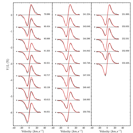
Figure 1: Time-series of Stokes $V$ profiles of AD Leo, in the rest-frame of the star, from our 2007 (left-hand column) and 2008 (middle and right-hand columns) data sets. Synthetic profiles corresponding to our magnetic models (red lines) are superimposed to the observed LSD profiles (black lines). Left to each profile a $\pm 1-\sigma$ error bar is shown. The rotational phase and cycle of each observation is also mentioned right to each profile. Successive profiles are shifted vertically for clarity purposes and the associated reference levels ($V=0$) are plotted as dotted lines.

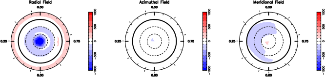
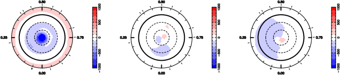
Figure 2: Surface magnetic flux of AD Leo as derived from our 2007 (upper row) and 2008 (lower row) data sets. The three components of the field in spherical coordinates are displayed from left to right (flux values labelled in G). The star is shown in flattened polar projection down to latitudes of $-30\hbox{${}^{\circ}$}$, with the equator depicted as a bold circle and parallels as dashed circles. Radial ticks around each plot indicate phases of observations.

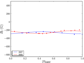
Figure 3: Longitudinal magnetic field of AD Leo as computed from the observed LSD Stokes $I$ and $V$ profiles for each observation epochs, 1-$\sigma$ error bars are also plotted (see Tab LABEL:tab:log_adleo). The solid lines represent the longitudinal field corresponding to the magnetic topologies reconstructed by ZDI and shown in Fig 2. The scale is the same for all the plots of longitudinal field.

We observed AD Leo in January-February 2007, and then one year later in January-February 2008 (see Tab. LABEL:tab:log_adleo). We respectively secured 9 and 14 spectra at each epoch (see Fig. 1) providing complete though not very dense coverage of the rotational cycle (see Fig. 2). Both time-series are very similar, we detect a strong signature of negative polarity (i.e. longitudinal field directed towards the star) exhibiting only very weak time-modulation (see Fig. 3). We thus expect that the star is seen nearly pole-on. We measure mean RV of $12.39~{}\hbox{km\,s${}^{-1}$}$ and $12.35~{}\hbox{km\,s${}^{-1}$}$ in 2007 and 2008 respectively, in good agreement with the value reported by Nidever et al. (2002) of $12.42\pm 0.1~{}\hbox{km\,s${}^{-1}$}$. The dispersion about these mean RV is equal to $0.04~{}\hbox{km\,s${}^{-1}$}$ at both epochs, i.e. close to the internal RV accuracy of NARVAL (about $0.03~{}\hbox{km\,s${}^{-1}$}$, see Sec. 3). These variations likely reflect the internal RV jitter of AD Leo since we observe a smooth variation of RV as a function of the rotational phase (even for observations occurring at different rotation cycles). We notice that RV and $B_{l}$ are in quadrature at both epochs. Given the previously reported stellar parameters $\hbox{$v\sin i$}=3.0~{}\hbox{km\,s${}^{-1}$}$ (Reiners & Basri, 2007), a rotation period of $2.7~{}\hbox{$\rm d$}$ (Spiesman & Hawley, 1986) and $\hbox{$R_{\star}$}\leq 0.40~{}\hbox{${\rm R}_{\odot}$}$ (see Tab. 1) we indeed infer $i\simeq 20\hbox{${}^{\circ}$}$.

We first process separately the 2007 and 2008 data described above with ZDI assuming $\hbox{$v\sin i$}=3.0~{}\hbox{km\,s${}^{-1}$}$, $i=20\hbox{${}^{\circ}$}$, and reconstruct modes up to order $\ell=8$, which is enough given the low rotational velocity of AD Leo. It is possible to fit the Stokes $V$ spectra down to $\hbox{$\chi^{2}_{r}$}=2.0$ (from an initial $\hbox{$\chi^{2}_{r}$}\simeq 250$) for both data sets if we assume $P_{ZDI}=2.22~{}\hbox{$\rm d$}$, which is significantly lower than the formerly estimated photometric period. Very similar results are obtained whether we assume that the field is purely poloidal or the presence a toroidal component. In the latter case toroidal fields only account for 5% of the overall recovered magnetic energy in 2008, whereas they are only marginally recovered from the 2007 – sparser – dataset (1%).

Very similar large-scale magnetic fields are recovered from both data sets (see Fig.2), with an average recovered magnetic flux $B\simeq 0.2~{}\hbox{$\rm kG$}$. We report a strong polar spot of radial field of maximum magnetic flux $B=1.3~{}\hbox{$\rm kG$}$ as the dominant feature of the surface magnetic field. The spherical harmonics decomposition of the surface magnetic field confirms what can be inferred from the magnetic maps. First, the prominent mode is the radial component of a dipole aligned with the rotational axis i.e. the $\ell=1,m=0$ mode of the radial component ($\alpha(1;0)$ contains more than 50% of the reconstructed magnetic energy). Secondly, the magnetic topology is strongly axisymmetric with about 90% of the energy in $m=0$ modes. Thirdly, among the recovered modes the lower order ones encompass most of the reconstructed magnetic energy ($\simeq 60\%$ in the dipole modes, i.e. modes $\alpha$ or $\beta$ modes of order $\ell=0$), though we cannot fit our data down to $\hbox{$\chi^{2}_{r}$}=2.0$ if we do not include modes up to order $\ell=8$.

We use ZDI to measure differential rotation as explained in Section 4.3. The $\chi^{2}_{r}$ map resulting from the analysis of the 2008 dataset does not features a clear paraboloid but rather a long valley with no well-defined minimum. If we assume solid-body rotation, a clear minimum is obtained at $\hbox{$P_{\rm rot}$}=2.24\pm 0.02~{}\hbox{$\rm d$}$ (3-$\sigma$ error-bar).

To estimate the degree at which the magnetic topology remained stable over 1 yr, we merge our 2007 and 2008 data sets together and try to fit them simultaneously with a single field structure. Assuming rigid-body rotation, it is possible to fit the complete data set down to $\hbox{$\chi^{2}_{r}$}=2.4$, demonstrating that intrinsic variability between January 2007 and January 2008 is detectable in our data though very limited. The corresponding rotation period is $\hbox{$P_{\rm rot}$}=2.2399\pm 0.0006~{}\hbox{$\rm d$}$ (3-$\sigma$ error-bar). We also find aliases for both shorter and longer periods, corresponding to shifts of $\sim 0.014~{}\hbox{$\rm d$}$. The nearest local minima located at $\hbox{$P_{\rm rot}$}=2.2264~{}\hbox{$\rm d$}$ and $\hbox{$P_{\rm rot}$}=2.2537~{}\hbox{$\rm d$}$, are associated with $\Delta\hbox{$\chi^{2}$}$ values of 36 and 31 respectively; the corresponding rotation rates are thus fairly excluded. The periods we find for the 2008 data set alone or for both data sets are compatible with each other. But they are not with the period reported by Spiesman & Hawley (1986) ($2.7\pm 0.05~{}\hbox{$\rm d$}$) based on 9 photometric measurements, for which we believe that the error bar was underestimated.

6 EV Lac = GJ 873 = HIP 112460

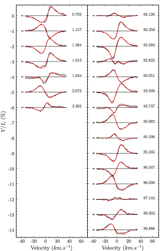
Figure 4: Same as Fig. 1 for EV Lac 2006 (left-hand column) and 2007 (right-hand column) data sets.

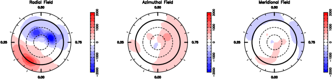
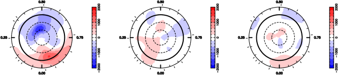
Figure 5: Same as Figure 2 for EV Lac, using data obtained in 2006 (upper row) and 2007 (lower row).

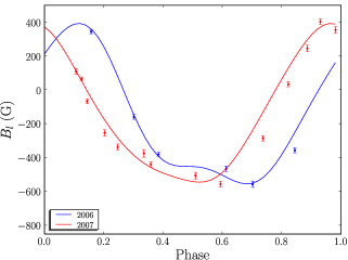
Figure 6: Same as Figure 3 for EV Lac.

EV Lac was observed in August 2006 and July-August 2007, we respectively obtained 7 and 15 spectra (see Tab. LABEL:tab:log_evlac and Fig. 4) providing complete though not very dense phase coverage (See Fig. 5) . We detect strong signatures in all the spectra and modulation is obvious for each time-series (see Fig. 6). We measure mean RV of $0.28~{}\hbox{km\,s${}^{-1}$}$ and $0.36~{}\hbox{km\,s${}^{-1}$}$ in 2006 and 2007 respectively, in good agreement with the value of $0.41\pm 0.1~{}\hbox{km\,s${}^{-1}$}$ reported by Nidever et al. (2002). The dispersion about these mean RV is equal to $0.13~{}\hbox{km\,s${}^{-1}$}$ at both epochs. These RV variations are smooth and correlate well with longitudinal fields in our 2007 data, but the correlation is less clear for 2006 (sparser) data. Assuming a rotation period of $4.378~{}\hbox{$\rm d$}$, determined photometrically by Pettersen (1980), and considering $\hbox{$v\sin i$}\simeq 3.0~{}\hbox{km\,s${}^{-1}$}$ (Reiners & Basri, 2007) or $\hbox{$v\sin i$}=4.5\pm 0.5~{}\hbox{km\,s${}^{-1}$}$ (Johns-Krull & Valenti, 1996), we straightforwardly deduce $\hbox{$R_{\star}$}~{}\sin i\simeq 0.35~{}\hbox{${\rm R}_{\odot}$}$. As $\hbox{$R_{\star}$}\simeq 0.30~{}\hbox{${\rm R}_{\odot}$}$, we expect a high inclination angle.

We use the above value for $P_{ZDI}$, $i=60\hbox{${}^{\circ}$}$, and perform a spherical harmonics decomposition up to order $\ell=8$. It is then possible to fit our Stokes $V$ 2007 data set from an initial $\hbox{$\chi^{2}_{r}$}=82$ down to $\hbox{$\chi^{2}_{r}$}=2.0$ for any velocity $3.0\leq\hbox{$v\sin i$}\leq 5.0~{}\hbox{km\,s${}^{-1}$}$. Neither the fit quality on Stokes $I$ spectra nor the properties of the reconstructed magnetic topology are significantly affected by the precise value of $v\sin i$, whereas the filling factors and the reconstructed magnetic flux are. The greater the velocity the lower the filling factors, and the average magnetic flux $B$ ranges from $0.5~{}\hbox{$\rm kG$}$ at $5.0~{}\hbox{km\,s${}^{-1}$}$ to $0.6~{}\hbox{$\rm kG$}$ at $3.0~{}\hbox{km\,s${}^{-1}$}$. Despite the fact that we achieve a poorer fit for the 2006 data set (from an initial $\hbox{$\chi^{2}_{r}$}=125$), $\hbox{$\chi^{2}_{r}$}=4.0$ for $\hbox{$v\sin i$}=5.0~{}\hbox{km\,s${}^{-1}$}$ and $\hbox{$\chi^{2}_{r}$}=4.5$ for $3.0~{}\hbox{km\,s${}^{-1}$}$, the same trends are observed. In the rest of the paper we assume $\hbox{$v\sin i$}=4.0~{}\hbox{km\,s${}^{-1}$}$ for EV Lac.

We recover simple and fairly similar magnetic topologies from both data sets (see Fig. 5). The surface magnetic field reconstructed from 2007 data is mainly composed of two strong spots of radial field of opposite polarities where magnetic flux $B$ reaches more than 1.5 $\rm kG$. The spots are located at opposite longitudes; the positive polarity being on the equator and the negative one around 50^∘ of latitude. The field is far from axisymmetry, as expected from the polarity reversal observed in Stokes $V$ signature during the rotation cycle (see Fig. 4). The 2006 topology differs by a rather stronger magnetic flux, maximum flux is above 2 $\rm kG$ with average flux stronger by 0.1 $\rm kG$ than in 2007; the spot of negative polarity is splitted into two distinct structures; and toroidal field is not negligible (in particular visible as spot of azimuthal field).

Magnetic energy is concentrated (60% in 2006, 75% in 2007) in the radial dipole modes $\alpha(1;0)$ and $\alpha(1;1)$, no mode of degree $\ell>1$ is above the 5% level, though fitting the data down to $\hbox{$\chi^{2}_{r}$}=2.0$ requires taking into account modes up to $\ell=8$. Toroidal field gathers more than 10% of the energy in 2006, whereas they are only marginally reconstructed (2%) in 2007. Although the magnetic distribution is clearly not axisymmetric, $m=0$ modes encompass approximately one third of the magnetic energy at both epochs.

We then try to constrain the surface differential rotation of EV Lac as explained in Section 4.3. The $\chi^{2}_{r}$ map computed from 2007 data can be fitted by a paraboloid. We thus infer the rotation parameters: $\hbox{$\Omega_{\rm eq}$}=1.4385\pm 0.0008~{}\hbox{rad\,d${}^{-1}$}$ and $\hbox{$d\Omega$}=1.7\pm 0.8~{}\hbox{mrad\,d${}^{-1}$}$. Our data are thus compatible with solid-body rotation within 3-$\sigma$. Assuming rigid rotation, we find a clear $\chi^{2}_{r}$ minimum for $\hbox{$P_{\rm rot}$}=4.37\pm 0.01~{}\hbox{$\rm d$}$ (3-$\sigma$ error-bar).

Although the magnetic topologies recovered from 2006 and 2007 are clearly different, they exhibit common patterns. We merge both data sets and try to fit them simultaneously with a single magnetic topology. Assuming solid-body rotation, we find a clear $\chi^{2}_{r}$ minimum for $\hbox{$P_{\rm rot}$}=4.3715\pm 0.0006~{}\hbox{$\rm d$}$ (3-$\sigma$ error-bar). We mention the formal error bar which may be underestimated since variability can have biased the rotation period determination. We also find aliases to shifts of $\sim 0.05~{}\hbox{$\rm d$}$, $\hbox{$P_{\rm rot}$}=4.3201~{}\hbox{$\rm d$}$ and $\hbox{$P_{\rm rot}$}=4.4248~{}\hbox{$\rm d$}$ for the nearest ones. With $\Delta\hbox{$\chi^{2}$}$ values of 2522 and 1032 these values are safely excluded. The periods we find for the 2007 data set alone or for both data sets are compatible with each other and in good agreement with the one reported by Pettersen (1980) and Pettersen et al. (1983) (4.378 and 4.375 $\rm d$) based on photometry.

7 YZ CMi = GJ 285 = HIP 37766

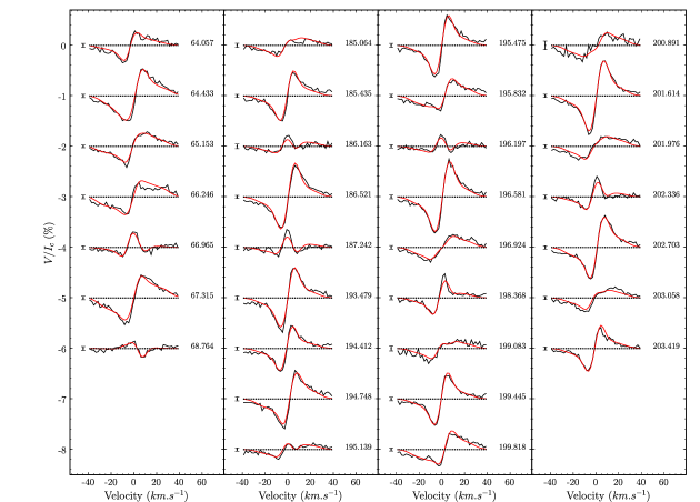
Figure 7: Same as Fig. 1 for YZ CMi 2006 (column 1) and 2007 (columns 2, 3 and 4) data sets.

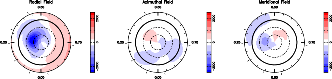
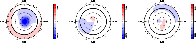
Figure 8: Same as Figure 2 for YZ CMi using data obtained in 2007 (upper row) and 2008 (lower row).

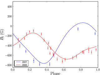
Figure 9: Same as Figure 3 for YZ CMi.

We collected 7 spectra of YZ CMi in January-February 2007 and 25 between December 2007 and February 2008 (see Tab. LABEL:tab:log_yzcmi and Fig. 7). For $P_{ZDI}=2.77~{}\hbox{$\rm d$}$ (Pettersen et al., 1983, photometry), we notice that the 2007 data provide correct phase coverage for half the rotation cycle only. On the opposite, the 2008 data provide complete and dense sampling of the rotational cycle (see Fig. 8). Rotational modulation is very clear for both data sets (see Fig. 9). We measure mean RV of $26.64~{}\hbox{km\,s${}^{-1}$}$ and $26.60~{}\hbox{km\,s${}^{-1}$}$ in 2007 and 2008 data set, respectively, in good agreement with $v_{r}=26.53\pm 0.1~{}\hbox{km\,s${}^{-1}$}$ reported by Nidever et al. (2002). The corresponding dispersions are $0.13~{}\hbox{km\,s${}^{-1}$}$ and $0.21~{}\hbox{km\,s${}^{-1}$}$, the difference likely reflects the poor phase coverage provided by 2007 data rather than an intrinsic difference. Although RV varies smoothly with the rotation phase, we do not find any obvious correlation between $B_{l}$ and RV. From the stellar mass (computed from $\rm M_{J}$, see Sec. 2), we infer $\hbox{$R_{\star}$}\simeq 0.30~{}\hbox{${\rm R}_{\odot}$}$. The above rotation period and $\hbox{$v\sin i$}=5~{}\hbox{km\,s${}^{-1}$}$ (Reiners & Basri, 2007) implies $\hbox{$R\sin i$}=0.27~{}\hbox{${\rm R}_{\odot}$}$ and thus a high inclination angle of the rotational axis.

We run ZDI on these Stokes $V$ time-series with the aforementioned values for $P_{ZDI}$ and $v\sin i$, and $i=60\hbox{${}^{\circ}$}$. Both data sets can be fitted from an initial $\hbox{$\chi^{2}_{r}$}\simeq 38$ down to $\hbox{$\chi^{2}_{r}$}=2.0$ using spherical harmonics decomposition up to order $\ell=6$. An average magnetic flux $B\simeq 0.6~{}\hbox{$\rm kG$}$ is recovered for both observation epochs.

The large-scale topology recovered from 2008 data is quite simple: the visible pole is covered by a strong spot of negative radial field (field lines penetrating the photosphere) – where the magnetic flux reaches up to 3 $\rm kG$ – while the other hemisphere is mainly covered by emerging field lines. Radial, and thus poloidal, field is widely prevailing, toroidal magnetic energy only stands for 3% of the whole. The magnetic field structure also exhibits strong axisymmetry, with about 90% of the magnetic energy in $m=0$ modes.

The main difference between 2007 and 2008 maps is that in 2007 this negative radial field spot is located at a lower latitude. We argue that this may be partly an artifact due to poor phase coverage. As only one hemisphere is observed the maximum entropy solution is a magnetic region facing the observer, rather than a stronger polar spot. We therefore conclude that non-axisymmetry inferred from 2007 observations is likely over-estimated.

We try a measurement of differential rotation from our time-series of Stokes $V$ spectra, as explained in Section 4.3. From our 2008 data set we obtain a $\chi^{2}_{r}$ map featuring a clear paraboloid. We infer the following rotation parameters: $\hbox{$\Omega_{\rm eq}$}=2.262\pm 0.001\hbox{rad\,d${}^{-1}$}$ and $\hbox{$d\Omega$}=0.0\pm 1.8~{}\hbox{mrad\,d${}^{-1}$}$. Assuming solid-body rotation, we derive $\hbox{$P_{\rm rot}$}=2.779\pm 0.004~{}\hbox{$\rm d$}$ (3-$\sigma$ error-bar).

We proceed as for AD Leo to estimate the intrinsic evolution of the magnetic topology between our 2007 and 2008 observations. Assuming rigid-body rotation, it is possible to fit the complete data set down to $\hbox{$\chi^{2}_{r}$}=3.9$ showing that definite – though moderate – variability occurred between the two observation epochs. The rotation period corresponding to the minimum $\chi^{2}_{r}$ is $\hbox{$P_{\rm rot}$}=2.7758\pm 0.0006~{}\hbox{$\rm d$}$ (3-$\sigma$ error-bar). The aliases (shifts of $\sim 0.021~{}\hbox{$\rm d$}$) can be safely excluded ($\Delta\hbox{$\chi^{2}$}=1450$ and 440 for $\hbox{$P_{\rm rot}$}=2.7546~{}\hbox{$\rm d$}$ and $2.7966~{}\hbox{$\rm d$}$, respectively). The periods we find for the 2008 data set alone or for both data sets are compatible with each other and with in good agreement the one reported by Pettersen et al. (1983) (2.77 $\rm d$) based on photometry.

8 EQ Peg A = GJ 896 A = HIP 116132

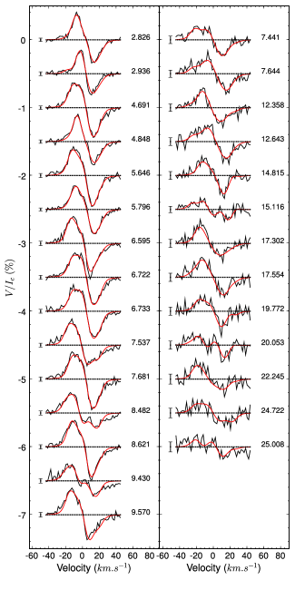
Figure 10: Same as Fig. 1 for EQ Peg A (left-hand column) and EQ Peg B (right-hand column) 2006 data sets

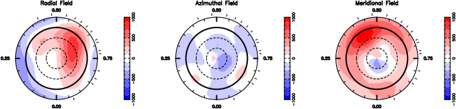
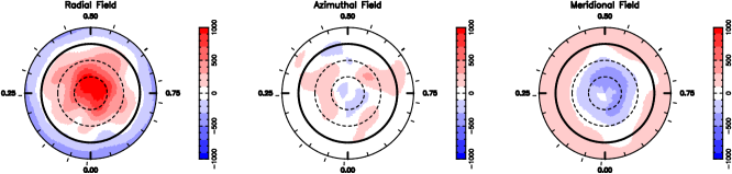
Figure 11: Same as Figure 2 for EQ Peg A (upper row) and B (lower row) as derived from our 2006 data sets.

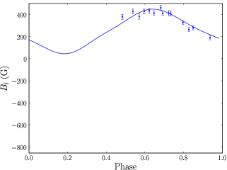
Figure 12: Same as Figure 3 for EQ Peg A.

We observed EQ Peg A in August 2006 and obtained a set of 15 Stokes $I$ and $V$ spectra (see Tab. LABEL:tab:log_eqpega and Fig. 10), providing observations of only one hemisphere of the star (see Fig. 11) considering $P_{ZDI}=1.06~{}\hbox{$\rm d$}$. Zeeman signatures are detected in all the spectra, showing moderate time-modulation (see Fig. 12). We measure a mean RV of $0.31~{}\hbox{km\,s${}^{-1}$}$ with a dispersion of $0.18~{}\hbox{km\,s${}^{-1}$}$. Although RV exhibits smooth variations along the rotational cycles, we do not find any simple correlation between RV and $B_{l}$. We find the best agreement between the LSD profiles and the model for $\hbox{$v\sin i$}=17.5~{}\hbox{km\,s${}^{-1}$}$. This implies $\hbox{$R_{\star}$}~{}\sin i\simeq 0.37~{}\hbox{${\rm R}_{\odot}$}$, whereas provided $\hbox{$M_{\star}$}=0.39\hbox{${\rm M}_{\odot}$}$ we infer $\hbox{$R_{\star}$}\simeq 0.35~{}\hbox{${\rm R}_{\odot}$}$. We thus assume $i=60\hbox{${}^{\circ}$}$ for ZDI calculations.

Stokes $V$ LSD time-series can be fitted from an initial $\hbox{$\chi^{2}_{r}$}=44$ down to $\hbox{$\chi^{2}_{r}$}=1.5$ using a spherical harmonics decomposition up to order $\ell=6$ by a field of average magnetic flux $B=0.5~{}\hbox{$\rm kG$}$. The recovered magnetic map (see Fig. 11), though exhibiting a similar structure of the radial component – one strong spot with $B=0.8~{}\hbox{$\rm kG$}$ – is more complex than those of previous stars, since we also recover significant azimuthal and meridional fields.

The field is dominated by large-scale modes: dipole modes encompass 70% of the overall magnetic energy and modes of order $\ell>2$ are all under the 2% level. Although poloidal field is greatly dominant, the toroidal component features 15% of the overall recovered magnetic energy. The magnetic topology is clearly not purely axisymmetric but the $m=0$ modes account for 70% of the reconstructed magnetic energy.

We use ZDI to measure differential rotation as explained in Section 4.3. We thus infer $\hbox{$\Omega_{\rm eq}$}=5.92\pm 0.02~{}\hbox{rad\,d${}^{-1}$}$ and $\hbox{$d\Omega$}=49\pm 43~{}\hbox{mrad\,d${}^{-1}$}$. This value is compatible with solid body rotation though the error bar is higher than for EV Lac and YZ CMi since data only span 1 week (rather than about 1 month for previous stars). Then assuming solid body rotation, we find $\hbox{$P_{\rm rot}$}=1.061\pm 0.004~{}d$ (3-$\sigma$ error-bar), which is in good agreement with the period of 1.0664 $\rm d$reported by Norton et al. (2007).

9 EQ Peg B = GJ 896 B

Figure 13: Same as Figure 3 for EQ Peg B.

EQ Peg B was observed in August 2006, we obtained a set of 13 Stokes $I$ and $V$ spectra (see Tab. LABEL:tab:log_eqpegb). Sampling of the star’s surface is almost complete (see Fig. 11) – and the derived $P_{ZDI}=0.405~{}\hbox{$\rm d$}$. Stokes $V$ signatures have a peak-to-peak amplitude above the 1-$\sigma$ noise level in all spectra, time-modulation is easily detected (see Fig. 10 and 13). We measure a mean RV of $3.34~{}\hbox{km\,s${}^{-1}$}$ with a dispersion of $0.16~{}\hbox{km\,s${}^{-1}$}$. RV is a soft function of the rotation phase, but we do not find obvious correlation between RV and $B_{l}$. We derive a rotational velocity $\hbox{$v\sin i$}=28.5~{}\hbox{km\,s${}^{-1}$}$ and thus $\hbox{$R\sin i$}=0.23~{}\hbox{${\rm R}_{\odot}$}$. From the measured J-band absolute magnitude, we infer $\hbox{$R_{\star}$}\simeq 0.25~{}\hbox{${\rm R}_{\odot}$}$, we will therefore assume $i=60\hbox{${}^{\circ}$}$.

A spherical harmonics decomposition up to order $\ell=8$ allows to fit the data from an initial $\hbox{$\chi^{2}_{r}$}=4.6$ down to $\hbox{$\chi^{2}_{r}$}=1.0$. Using higher order modes does not result in significant changes. Due to the high rotational velocity, we find similar results for any value $0<f_{V}<1$.

The reconstructed magnetic map (see Fig. 11) exhibits a very simple structure: the hemisphere oriented toward the observer is mainly covered by positive (emerging) radial fields, in particular a strong spot ($B=1.2~{}\hbox{$\rm kG$}$) lies close to the pole; the other hemisphere is covered by negative radial fields. The meridional component has the same structure as found for V374 Peg (M08). Except the (weak) azimuthal component the recovered magnetic topology is strongly axisymmetric. The average magnetic flux is $B\simeq 0.4~{}\hbox{$\rm kG$}$.

As obvious from Fig. 11 the mode $\alpha(1;0)$ is dominant, it encompasses 75% of the magnetic energy whereas no other mode is stronger than 7%. The field is mostly axisymmetric with about 90% of the magnetic energy in $m=0$ modes, and mostly poloidal ($>95\%$).

Using the method described in Section 4.3, we produce a map of the $\chi^{2}_{r}$ as a function of the rotation parameters $\Omega_{\rm eq}$ and $d\Omega$ featuring no clear minimum in a reasonable range of values. This may due to a poor constraint on differential rotation since our data set only span 1 week, and the magnetic topology is mainly composed of one polar spot. Assuming solid body rotation, we find $\hbox{$P_{\rm rot}$}=0.404\pm 0.004~{}d$ (3-$\sigma$ error-bar).

10 Discussion and conclusion

Table 7: Magnetic quantities derived from our study. For each star, different observation epochs are presented separately. In columns 2–5 we report quantities from Table 1, respectively the stellar mass, the rotation period (with an accuracy of 2 digits), the effective Rossby number and the X-ray to bolometric luminosity ratio. Columns 6, 7 and 8 mention the Stokes $V$ filling factor, the reconstructed magnetic energy and the average magnetic flux. Columns 9–13 list the percentage of reconstructed magnetic energy respectively lying in poloidal, dipole (poloidal and $\ell=1$), quadrupole (poloidal and $\ell=2$), octupole (poloidal and $\ell=3$) and axisymmetric modes ($m=0$ / $m<\ell/2$).

Name	Mass	$P_{\rm rot}$	$Ro$	log$R_{X}$	$f_{V}$	$<B^{2}>$	$<B>$	pol.	dipole	quad.	oct.	axisymm.
	(${\rm M}_{\odot}$)	(d)	($10^{-2}$)			($\rm 10^{5}\,G^{2}$)	(kG)	(%)	(%)	(%)	(%)	(%)
EV Lac (06)	0.32	4.38	6.8	-3.3	0.11	4.48	0.57	87	60	13	3	33/36
EV Lac (07)	–	–	–	–	0.10	3.24	0.49	98	75	10	3	28/31
YZ CMi (07)	0.31	2.77	4.2	-3.1	0.11	5.66	0.56	92	69	10	5	56/61
YZ CMi (08)	–	–	–	–	0.11	4.75	0.55	97	72	11	8	85/86
AD Leo (07)	0.42	2.24	4.7	-3.2	0.14	0.61	0.19	99	56	12	5	95/97
AD Leo (08)	–	–	–	–	0.14	0.61	0.18	95	63	9	3	85/88
EQ Peg A (06)	0.39	1.06	2.0	-3.0	0.11	2.73	0.48	85	70	6	6	69/70
EQ Peg B (06)	0.25	0.40	0.5	-3.3	na	2.38	0.45	97	79	8	5	92/94
V374 Peg (05)	0.28	0.45	0.6	-3.2	na	6.55	0.78	96	72	12	7	75/76
V374 Peg (06)	–	–	–	–	na	4.60	0.64	96	70	17	4	76/77

Figure 14: Properties of the magnetic topologies of M dwarfs as a function of rotation period and stellar mass. Larger symbols indicate larger magnetic fields while symbol shapes depict the different degrees of axisymmetry of the reconstructed magnetic field (from decagons for purely axisymmetric fields to sharp stars for purely non axisymmetric fields). Colours illustrate the field configuration (dark blue for purely toroidal fields, dark red for purely poloidal fields and intermediate colours for intermediate configurations). Solid lines represent contours of constant Rossby number $Ro=0.1$ and $0.01$ respectively corresponding approximately to the saturation and super-saturation thresholds (e.g., Pizzolato et al., 2003). The theoretical full-convection limit ($\hbox{$M_{\star}$}\simeq 0.35\hbox{${\rm M}_{\odot}$}$, Chabrier & Baraffe 1997) is plotted as a horizontal dashed line.

Spectropolarimetric observations of a small sample of active M dwarfs around spectral type M4 were carried out with ESPaDOnS at CFHT and NARVAL at TBL between 2006 Jan and 2008 Feb. Strong Zeeman signatures are detected in Stokes $V$ spectra for all the stars of the sample. Using ZDI, with a Unno-Rachkovsky’s model modified by two filling factors, we can fit our Stokes $V$ time series. It can be seen on Fig. 1, 4, 7 and 10 that rotational modulation is indeed mostly modelled by the imaging code.

From the resulting magnetic maps, we find that the observed stars exhibit common magnetic field properties. (a) We recover mainly poloidal fields, in most stars the observations can be fitted without assuming a toroidal component. (b) Most of the energy is concentrated in the dipole modes, i.e. the lowest order modes. (c) The purely axisymmetric component of the field ($m=0$ modes) is widely dominant except in EV Lac. These results confirm the findings of M08, i.e. that magnetic topologies of fully-convective stars considerably differ from those of warmer G and K stars which usually host a strong toroidal component in the form of azimuthal field rings roughly coaxial with the rotation axis (e.g., Donati et al., 2003a).

Table LABEL:tab:syn gathers the main properties of the reconstructed magnetic fields and Figure 14 presents them in a more visual way. We can thus suspect some trends: (a) The only partly-convective stars of the sample, AD Leo, hosts a magnetic field with similar properties to the observed fully-convective stars. The only difference is that compared to fully-convective stars of similar $Ro$, we recover a significantly lower magnetic flux on AD Leo, indicating that the generation of a large-scale magnetic field is more efficient in fully-convective stars. This will be confirmed in a future paper by analysing the early M stars of our sample. (b) We do not observe a growth of the reconstructed large-scale magnetic flux with decreasing Rossby number, thus suggesting that dynamo is already saturated for fully-convective stars having rotation periods lower than 5 $\rm d$, in agreement with Pizzolato et al. (2003) and Kiraga & Stepien (2007). Further confirmation from stars with $\hbox{$P_{\rm rot}$}\gtrsim 10~{}\hbox{$\rm d$}$ is needed. This is supported by the high X-ray fluxes we report, all lying in the saturated part of the rotation-activity relation with log$R_{X}\simeq-3$ (e.g., James et al., 2000). AD Leo also exhibits a saturated X-ray luminosity despite a significantly weaker reconstructed magnetic field, indicating that the coronal heating is not directly driven by the large-scale magnetic field. (c) The only star showing strong departure from axisymmetry is EV Lac, i.e. the slowest rotator (though lying in the saturated regime with $Ro=0.07$). Further investigation is needed to check if this a general result for fully-convective stars having $\hbox{$P_{\rm rot}$}\gtrsim 4~{}\hbox{$\rm d$}$.

The large-scale magnetic fluxes we report here range from 0.2 to 0.8 $\rm kG$. For AD Leo, EV Lac and YZ CMi, previous measurements from Zeeman broadening of atomic or molecular unpolarised line profiles report significantly higher overall magnetic fluxes (several $\rm kG$) (e.g., Saar & Linsky, 1985; Johns-Krull & Valenti, 1996; Reiners & Basri, 2007). We therefore conclude that a significant part of the magnetic energy lies in small-scale fields. Even for the fast rotators EQ Peg A and B and V374 Peg for which ZDI is sensitive to scales corresponding to spherical harmonics up to order $\ell=\,$12, 20 and 25 (cf. M08), respectively, we reconstruct a large majority of the magnetic energy in modes of order $\ell\leq 3$. This suggests that the magnetic features we miss with ZDI lie at scales corresponding to $\ell>25$ in the reconstructed magnetic fields of mid-M dwarfs.

Three stars of the sample have been observed at two different epochs separated by about 1 yr. AD Leo, EV Lac, and YZ CMi exhibit only faint variations of their magnetic topology during this time gap, the overall magnetic configuration remained stable similarly to the behaviour of V374 Peg (cf. M08). This is at odds with what is observed in more massive active stars, whose magnetic fields reportedly evolve significantly on time-scales of only a few months (e.g., Donati et al., 2003a).

For three stars of our sample we are able to measure differential rotation and find that our data are compatible with solid-body rotation. In addition, for EV Lac and YZ CMi we infer that differential rotation is at most of the order of a few mrad d^-1 i.e. significantly weaker than in the Sun and apparently lower than in V374 Peg (cf. M08). This is further confirmed by the fact that the rotation periods we find are in good agreement with photometric periods previously published in the literature (whenever reliable).

This result is consistent with the conclusions of the latest numerical dynamo simulations in fully convective dwarfs with $Ro\simeq 0.01$ (Browning, 2008) showing that (i) strong magnetic fields are efficiently produced throughout the whole star (with the magnetic energy being roughly equal to the convective kinetic energy as expected from strongly helical flows, i.e., with small $Ro$) and that (ii) these magnetic fields successfully manage to quench differential rotation to less than a tenth of the solar shear (as a result of Maxwell stresses opposing the equatorward transport of angular momentum due to Reynolds stresses). However, these simulations predict that dynamo topologies of fully convective dwarfs should be mostly toroidal, in contradiction with our observations showing strongly poloidal fields in all stars of the sample; the origin of this discrepancy is not clear yet.

Our study of Stokes $I$ and $V$ time-series allows to measure both the rotational period ($P_{\rm rot}$) and the projected equatorial velocity ($v\sin i$) of the sample, from which we can straightforwardly deduce the $R\sin i$. $P_{\rm rot}$ is well constrained by our data sets (see the error-bars in Tab. 1), therefore the incertitude on $R\sin i$ essentially comes from the determination of $v\sin i$ ($\sigma\simeq 1~{}\hbox{km\,s${}^{-1}$}$). This leads to an important incertitude on the $R\sin i$ deduced for slowly rotating stars. As explained in M08, for V374 Peg we find a $R\sin i$ significantly greater than the predicted radius . Here (except for AD Leo which is seen nearly pole-on) we find $\hbox{$R\sin i$}\simeq\hbox{$R_{\star}$}$ (cf. Tab. 1), suggesting radii larger than the predicted ones. This is consistent with the findings of Ribas (2006) on eclipsing binaries, further confirmed on a sample of single late-K and M dwarfs by Morales et al. (2008), that active low-mass stars exhibit significantly larger radii and cooler $T_{\rm eff}$ than inactive stars of similar masses. Chabrier et al. (2007) proposed in a phenomenological approach that a strong magnetic field may inhibit convection and produce the observed trends. This back-reaction of the magnetic field on the star’s internal structure may be associated with the dynamo saturation observed in our sample (see above), and with the frozen differential rotation predicted by Browning (2008) when the magnetic energy reaches equipartition (with respect to the kinetic energy).

We also detect significant RV variations in our sample (with peak-to-peak amplitude of up to 700 m s^-1). We observe the largest RV variations on the star having the strongest large-scale magnetic field (YZ CMi). This suggests that although the relation between magnetic field measurements and RV is not yet clear, these smooth fluctuations in RV are due to the magnetic field and the associated activity phenomena. Therefore, if we can predict the RV jitter due to a given magnetic configuration, spectropolarimetry may help in refining RV measurements of active stars, thus allowing to detect planets orbiting around M dwarfs.

The study presented through this paper aims at exploring the magnetic field topologies of a small sample of very active mid-M dwarfs, i.e. stars with masses close the full-convection threshold. Forthcoming papers will extend this work to both earlier (partly-convective) and later M dwarfs, in order to provide an insight on the evolution of magnetic topologies with stellar properties (mainly mass and rotation period). We thus expect to provide new constraints and better understanding of dynamo processes in both fully and partly convective stars.

References

- Babcock (1961) Babcock H. W., 1961, ApJ, 133, 572
- Baraffe et al. (1998) Baraffe I., Chabrier G., Allard F., Hauschildt P. H., 1998, A&A, 337, 403
- Barnes et al. (2005) Barnes J. R., Cameron A. C., Donati J.-F., James D. J., Marsden S. C., Petit P., 2005, MNRAS, 357, L1
- Brown et al. (1991) Brown S. F., Donati J.-F., Rees D. E., Semel M., 1991, A&A, 250, 463
- Browning (2008) Browning M. K., 2008, ApJ, 676, 1262
- Chabrier & Baraffe (1997) Chabrier G., Baraffe I., 1997, A&A, 327, 1039
- Chabrier et al. (2007) Chabrier G., Gallardo J., Baraffe I., 2007, A&A, 472, L17
- Chabrier & Küker (2006) Chabrier G., Küker M., 2006, A&A, 446, 1027
- Chandrasekhar (1961) Chandrasekhar S., 1961, Hydrodynamic and hydromagnetic stability. International Series of Monographs on Physics, Oxford: Clarendon, 1961
- Charbonneau (2005) Charbonneau P., 2005, Living Reviews in Solar Physics, 2, 2
- Claret (2004) Claret A., 2004, A&A, 428, 1001
- Cutri et al. (2003) Cutri R. M., Skrutskie M. F., van Dyk S., Beichman C. A., Carpenter J. M., Chester T., Cambresy L., Evans T., Fowler J., Gizis J., Howard E., Huchra J., Jarrett T., Kopan E. L., Kirkpatrick J. D., Light R. M., Marsh K. A., McCallon 2003, 2MASS All Sky Catalog of point sources.. The IRSA 2MASS All-Sky Point Source Catalog, NASA/IPAC Infrared Science Archive. http://irsa.ipac.caltech.edu/applications/Gator/
- Delfosse et al. (1998) Delfosse X., Forveille T., Perrier C., Mayor M., 1998, A&A, 331, 581
- Delfosse et al. (2000) Delfosse X., Forveille T., Ségransan D., Beuzit J.-L., Udry S., Perrier C., Mayor M., 2000, A&A, 364, 217
- Dobler et al. (2006) Dobler W., Stix M., Brandenburg A., 2006, ApJ, 638, 336
- Donati (2003c) Donati J.-F., 2003c, in Trujillo-Bueno J., Sanchez Almeida J., eds, Astronomical Society of the Pacific Conference Series Vol. 307 of Astronomical Society of the Pacific Conference Series, ESPaDOnS: An Echelle SpectroPolarimetric Device for the Observation of Stars at CFHT. pp 41–+
- Donati & Brown (1997b) Donati J.-F., Brown S. F., 1997b, A&A, 326, 1135
- Donati et al. (2003a) Donati J.-F., Cameron A., Semel M., Hussain G., Petit P., Carter B., Marsden S., Mengel M., Lopez Ariste A., Jeffers S., Rees D., 2003a, MNRAS, 345, 1145
- Donati et al. (2003b) Donati J.-F., Collier Cameron A., Petit P., 2003b, MNRAS, 345, 1187
- Donati et al. (2006) Donati J.-F., Forveille T., Cameron A. C., Barnes J. R., Delfosse X., Jardine M. M., Valenti J. A., 2006, Science, 311, 633
- Donati et al. (2006) Donati J.-F., Howarth I. D., Jardine M. M., Petit P., Catala C., Landstreet J. D., Bouret J.-C., Alecian E., Barnes J. R., Forveille T., Paletou F., Manset N., 2006, MNRAS, 370, 629
- Donati et al. (2008) Donati J.-F., Jardine M. M., Gregory S. G., Petit P., Paletou F., Bouvier J., Dougados C., Ménard F., Cameron A. C., Harries T. J., Hussain G. A. J., Unruh Y., Morin J., Marsden S. C., Manset N., Aurière M., Catala C., Alecian E., 2008, MNRAS, 386, 1234
- Donati et al. (1997a) Donati J.-F., Semel M., Carter B. D., Rees D. E., Cameron A. C., 1997a, MNRAS, 291, 658
- Donati et al. (2001) Donati J.-F., Wade G., Babel J., Henrichs H., de Jong J., Harries T., 2001, MNRAS, 326, 1256
- Durney et al. (1993) Durney B. R., De Young D. S., Roxburgh I. W., 1993, Solar Physics, 145, 207
- ESA (1997) ESA 1997, VizieR Online Data Catalog, 1239, 0
- James et al. (2000) James D. J., Jardine M. M., Jeffries R. D., Randich S., Collier Cameron A., Ferreira M., 2000, MNRAS, 318, 1217
- Johns-Krull & Valenti (1996) Johns-Krull C. M., Valenti J. A., 1996, ApJL, 459, L95+
- Joy & Humason (1949) Joy A. H., Humason M. L., 1949, PASP, 61, 133
- Kiraga & Stepien (2007) Kiraga M., Stepien K., 2007, ArXiv e-prints, 707
- Küker & Rüdiger (2005) Küker M., Rüdiger G., 2005, Astronomische Nachrichten, 326, 265
- Kurucz (1993) Kurucz R., 1993, CDROM # 13 (ATLAS9 atmospheric models) and # 18 (ATLAS9 and SYNTHE routines, spectral line database). Smithsonian Astrophysical Observatory, Washington D.C.
- Landi degl’Innocenti (1992) Landi degl’Innocenti E., 1992, Magnetic field measurements. Solar Observations: Techniques and Interpretation, pp 71–+
- Larmor (1919) Larmor J., 1919, Rep. Brit. Assoc. Adv. Sci.
- Leighton (1969) Leighton R. B., 1969, ApJ, 156, 1
- Lovell et al. (1963) Lovell B., Whipple F. L., Solomon L. H., 1963, Nature, 198, 228
- Mohanty & Basri (2003) Mohanty S., Basri G., 2003, ApJ, 583, 451
- Morales et al. (2008) Morales J. C., Ribas I., Jordi C., 2008, A&A, 478, 507
- Morin et al. (2008) Morin J., Donati J.-F., Forveille T., Delfosse X., Dobler W., Petit P., Jardine M. M., Cameron A. C., Albert L., Manset N., Dintrans B., Chabrier G., Valenti J. A., 2008, MNRAS, 384, 77
- Moutou et al. (2007) Moutou C., Donati J.-F., Savalle R., Hussain G., Alecian E., Bouchy F., Catala C., Collier Cameron A., Udry S., Vidal-Madjar A., 2007, A&A, 473, 651
- Nidever et al. (2002) Nidever D. L., Marcy G. W., Butler R. P., Fischer D. A., Vogt S. S., 2002, ApJS, 141, 503
- Norton et al. (2007) Norton A. J., Wheatley P. J., West R. G., Haswell C. A., Street R. A., Collier Cameron A., Christian D. J., Clarkson W. I., Enoch B., Gallaway M., Hellier C., Horne K., Irwin J., Kane S. R., Lister T. A., Nicholas J. P., Parley 2007, A&A, 467, 785
- Noyes et al. (1984) Noyes R. W., Hartmann L. W., Baliunas S. L., Duncan D. K., Vaughan A. H., 1984, ApJ, 279, 763
- Parker (1955) Parker E. N., 1955, ApJ, 122, 293
- Petit et al. (2002) Petit P., Donati J.-F., Cameron A., 2002, MNRAS, 334, 374
- Pettersen (1980) Pettersen B. R., 1980, AJ, 85, 871
- Pettersen et al. (1983) Pettersen B. R., Kern G. A., Evans D. S., 1983, A&A, 123
- Pizzolato et al. (2003) Pizzolato N., Maggio A., Micela G., Sciortino S., Ventura P., 2003, A&A, 397, 147
- Rees & Semel (1979) Rees D. E., Semel M. D., 1979, A&A, 74, 1
- Reid et al. (1995) Reid I. N., Hawley S. L., Gizis J. E., 1995, AJ, 110, 1838
- Reiners & Basri (2006) Reiners A., Basri G., 2006, ApJ, 644, 497
- Reiners & Basri (2007) Reiners A., Basri G., 2007, ApJ, 656, 1121
- Ribas (2006) Ribas I., 2006, Ap&SS, 304, 89
- Robrade et al. (2004) Robrade J., Ness J.-U., Schmitt J. H. M. M., 2004, A&A, 413, 317
- Saar (1988) Saar S. H., 1988, ApJ, 324, 441
- Saar & Linsky (1985) Saar S. H., Linsky J. L., 1985, ApJ, 299, L47
- Skilling & Bryan (1984) Skilling J., Bryan R. K., 1984, MNRAS, 211, 111
- Spiesman & Hawley (1986) Spiesman W. J., Hawley S. L., 1986, AJ, 92, 664
- Tamazian et al. (2006) Tamazian V. S., Docobo J. A., Melikian N. D., Karapetian A. A., 2006, PASP, 118, 814
- Unno (1956) Unno W., 1956, PASJ, 8, 108
- Wade et al. (2000) Wade G. A., Donati J.-F., Landstreet J. D., Shorlin S. L. S., 2000, MNRAS, 313, 851
- West et al. (2004) West A. A., Hawley S. L., Walkowicz L. M., Covey K. R., Silvestri N. M., Raymond S. N., Harris H. C., Munn J. A., McGehee P. M., Ivezić Ž., Brinkmann J., 2004, AJ, 128, 426