Comprehensive quantum Monte Carlo study of the quantum critical points in planar dimerized/quadrumerized Heisenberg models

Abstract

We study two planar square lattice Heisenberg models with explicit dimerization or quadrumerization of the couplings in the form of ladder and plaquette arrangements. We investigate the quantum critical points of those models by means of (stochastic series expansion) quantum Monte Carlo simulations as a function of the coupling ratio $\alpha=J^{\prime}/J$. The critical point of the order-disorder quantum phase transition in the ladder model is determined as $\alpha_{\mathrm{c}}=1.9096(2)$ improving on previous studies. For the plaquette model, we obtain $\alpha_{\mathrm{c}}=1.8230(2)$ establishing a first benchmark for this model from quantum Monte Carlo simulations. Based on those values, we give further convincing evidence that the models are in the three-dimensional (3D) classical Heisenberg universality class. The results of this contribution shall be useful as references for future investigations on planar Heisenberg models such as concerning the influence of non-magnetic impurities at the quantum critical point.

I Introduction

The study of quantum effects in magnetism is an ongoing and fascinating part of physics research.Schollwöck et al. (2004); Sachdev (2008) Within this area, the low-dimensional $S=1/2$ Heisenberg antiferromagnet plays an eminent role. This is partly because it correctly describes aspects of cuprate superconductors and is thus implemented in nature. Second, the Heisenberg model and variations have seen a lot of investigations as toy models where quantum fluctuations lead to unexpectedly rich and exotic ground-states (such as valence bond solids and valence bond liquids). Recent experiments in optical latticesTrotzky et al. (2008) further provide the perspective to directly implement those models in a pure environment thereby enabling a direct experimental access and comparison between theory and measurements.

In two-dimensional (2D) Heisenberg models, the Mermin-Wagner theorem forbids phase transitions to occur at $T\neq 0$, yet quantum fluctuations may lead to a transition between ground states, for example from an ordered Néel to a disordered state at zero temperature. Such transitions are termed quantum phase transitions.Sachdev (1999); Vojta (2003) One way in which quantum fluctuations can destroy order is for example provided via frustration of bonds (next-nearest-neighbor couplings) or the inclusion of 4-site interactions.Sandvik (2007)

In a second mechanism, competition between locally varying nearest-neighbor bonds of the same kind has been identified to cause quantum phase transitions, for example by favoring the formation of spin singlets. An important class of models in which the latter mechanism is at work are the so called dimerized Heisenberg models (where we also use the term for extended models with quadrumerization, etc.), where the competition among couplings is explicitly introduced in a geometric manner. Apart from their relevance as simple models for quantum phase transitions such systems have been in recent focus in connection with Bose-Einstein condensation of magnons.Giamarchi et al. (2008) A prominent example of dimerized models is the $S=1/2$ bilayer Heisenberg system Sandvik and Scalapino (1994); Sandvik et al. (1995); Troyer and Sachdev (1998); Shevchenko et al. (2000); Collins and Hamer (2008) which consists of two $L\times L$ layers, where the inter-layer coupling $J_{\perp}$ can be different from the intra-layer coupling $J$ (both couplings antiferromagnetic). Competition between $J_{\perp}$ and $J$ can drive a quantum phase transition.

Due to progress and availability of unbiased and efficient methodological schemesEvertz (2003) some numerical contributions in the literature were lately pushing results on those bilayer systems to unprecedented accuracy for quantum models, allowing for very detailed studies in the quantum critical regime. Following the high precision study on two bilayer systems by Wang et al.,Wang et al. (2006) Höglund and Sandvik could for example report on anomalous responseHöglund and Sandvik (2007) of non-magnetic impurities, for which an accurate knowledge of the quantum critical point was a prerequisite. The overall interest on such impurity based questions is growing,Sachdev et al. (1999); Anfuso and Eggert (2006); Sushkov (2000) therefore asking for the general availability of more detailed data also in other systems.

While the level of accuracy has reached a very high quality for bilayer systems, this is not equally the case for planar geometries. After the seminal simulation of the CaVO lattice by Troyer et al.,Troyer et al. (1997) only the coupled ladder model was considered in more detailMatsumoto et al. (2001) using quantum Monte Carlo (QMC) studies. A main result of these investigations was the confirmation of the critical exponents predicted by field theory.ChakravartyPRL ; Chubukov et al. (1994)

In an effort to systematically improve and extend these results to other planar Heisenberg models, we have recently started with a contributionWenzel et al. (2008a) reporting on peculiar and non-universal features of a particular dimerized model, called the $J-J^{\prime}$ or staggered model.Ivanov et al. (1996); Singh et al. (1988); Krüger et al. (2000); Tomczak and Richter (2001); Darradi et al. (2004) In Ref. Wenzel et al., 2008a, our presentation is based on a detailed scaling analysis at criticality and a comparison between several dimerized models including bilayer and planar geometries. As a prerequisite to this comparison, we have also presented new but preliminary results on the ladder and plaquette Heisenberg model without showing any details of our numerical data nor its data analysis. An in-depth study of these models on its own is, however, useful for several reasons. Apart from the aforementioned motivation concerning impurities, new benchmark results shall be useful for thermodynamic considerations in the quantum critical regime and for further developing and testing novel algorithms and numerical techniques.

In order to close this existing gap, we consider in this paper the critical points of the ladder and plaquette models defined by the Hamiltonian

$$\mathcal{H}=J\sum_{\langle i,j\rangle}\mathbf{S}_{i}\mathbf{S}_{j}+J^{\prime}\sum_{\langle i,j\rangle^{\prime}}\mathbf{S}_{i}\mathbf{S}_{j}\,.$$ (1)

Here, $\mathbf{S}_{i}=(1/2)\,(\sigma_{x},\sigma_{y},\sigma_{z})$ denotes the usual spin-$1/2$ operator at lattice site $i$, and $J$ and $J^{\prime}$ the antiferromagnetic coupling constants defined on bonds $\langle i,j\rangle$ and $\langle i,j\rangle^{\prime}$, respectively. The arrangements of the bonds on the square lattice of size $L$ in both directions can be seen in Fig. 1.

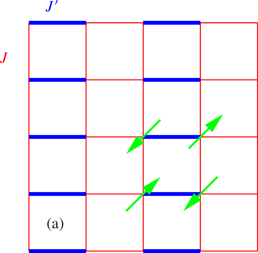
Figure 1: (Color online) (a) Visualization of the ladder model on the two-dimensional square lattice. The quantum spin ($S=1/2$) degrees of freedom live on a square lattice with different nearest-neighbour couplings $J$ and $J^{\prime}$ (thin and thick bonds). The lattice bonds corresponding to couplings $J^{\prime}$ are denoted as $\langle i,j\rangle^{\prime}$ in the Hamiltonian. (b) Similar for the plaquette model, favoring quadrumer formation. Both systems are studied using periodic boundary conditions.

Let us define the quantity $\alpha=J^{\prime}/J$ as the ratio of the two competing couplings. For $\alpha>\alpha_{\mathrm{c}}>1$ the systems will be disordered and gaped due to formation of spin-singlets. For $\alpha_{l}<\alpha<\alpha_{\mathrm{c}}$ the systems possess Néel order and there is no gap. Here $\alpha_{l}$ is some lower boundary at which a second transition can take place. In this regard, it is interesting to note that long range Néel order even for $\alpha=1$ was only recently established rigorously.Löw (2007) With $\alpha_{\mathrm{c}}$ we denote the quantum critical point. Throughout this work we fix $J=1$ and study the transition from the Néel to a disordered state, when $\alpha$ (or $J^{\prime}$) is increased.

Let us first summarize some previous work on the subject. Early contributions on the ladder model were done by Singh et al.,Singh et al. (1988) who used series expansions to access the critical point. Numerically oriented work followed from Katoh and ImadaKatoh and Imada (1993) and was later improved by Matsumoto et al.Matsumoto et al. (2001) in a detailed QMC study which had its major objective in studying the $S=1$ case. For $S=1/2$, to our knowledge the best known value for the critical coupling is taken from that paper as $\alpha_{\mathrm{c}}=1.9107(2)$ (which is the inverse of $0.52337(3)$), together with an estimate of the critical exponent $\nu=0.71(3)$. The latter result is often used/quoted in favor of $O(3)$ universality based on field theory. The $S=1/2$ ladder model has been further investigated in three dimensions (3D) in connection with field induced phenomena and Bose condensation of magnons.Nohadani et al. (2005, 2004) The effects of random site dilution in the dimerized phase were also studied.Yasuda et al. (2001) Quite generally, the coupled ladder model is nowadays often used as a paradigmatic model in discussions of quantum phase transitions and quantum magnetism.Sachdev (2008); Senthil et al. (2005)

Less is known about the plaquette model, which was studied before mainly analytically or with series expansions.Koga et al. (1999); Sirker et al. (2002); Singh et al. (1999) A recent study on the quadrumerized Shastry-Sutherland-modelLäuchli et al. (2002), using mainly exact diagonalization methods, also contains a (hidden) QMC estimate of the critical coupling $\alpha_{c}\approx 1.82$ for the pure plaquette model. Additionally, the plaquettized model returned into focus using a numerical scheme called contractor renormalization (CORE) method.Capponi et al. (2004) Still, it lacks a detailed quantum Monte Carlo investigation as presented in this paper.

The reason to reconsider the ladder model is threefold. First, we like to test our algorithm and approach on known models. Our second motivation is to complement the description of the phase transition in the ladder model beyond to what was done earlier. This includes the extension to different critical quantities, inclusion of corrections in the finite-size scaling analysis and calculation of critical exponents not considered before. Our aim is also to make the value of $\nu$ more accurate for definite interpretation in favor of $O(3)$ universality. Lastly, a major objective is to derive results which we partly presented in Ref. Wenzel et al., 2008a, as the dimerized ladder model is so similar to the staggered model.

We organize our paper as follows. In Sec. II we shortly present our implementation of the QMC method and data-analysis approaches. Standard observables used to detect the critical point are defined and discussed. A detailed presentation of our numerical data with a focus on the critical point is given in Sec. III. Section IV contains a finite-size scaling analysis of the critical exponents and a summary is given in Sec. V.

II Simulation methods and finite- size scaling

II.1 Quantum Monte Carlo simulations

In this work, we report on simulations based on our implementation of the stochastic series expansion (SSE) method by Sandvik and Kurkijärvi.Sandvik and Kurkijärvi (1991) Due to its discrete nature, this QMC scheme is a convenient and powerful method to implement. The central idea of SSE is to sample the series expansion of the partition function

$$Z=\mathrm{tr}\left[\exp(-\beta\mathcal{H})\right]=\sum_{\alpha}\sum_{n}\frac{(-\beta)^{n}\langle\alpha|\mathcal{H}^{n}|\alpha\rangle}{n!}\,,$$ (2)

with $n$ being the expansion order, $|\alpha\rangle$ a basis state of the spin space, and $\beta$ the inverse temperature. While the original algorithm used local Metropolis-type updates, major improvements were achieved by introducing cluster or operator loop updates.Sandvik (1999) Our own implementation is based on the directed loopSyljuåsen and Sandvik (2002) generalization together with additional ideas described by Alet et al..Alet et al. (2005) The recent incorporation of the Wang-Landau methodWang and Landau (2001) into the SSE schemeTroyer et al. (2003) allows the use of multihistogram techniques on QMC data A. M. Ferrenberg and R. Swendsen (1989); Troyer et al. (2004) which is useful to obtain unbiased continuous curves through data points, a feature which we use partly in our data analysis.

In order to access zero temperature properties of the spin system, all simulations must be performed at sufficiently large $\beta$ so that quantities of interest assume their ground-state value. In this contribution this is done in a two stage procedure. For a chosen lattice size, we check explicit convergence of observables by a $\beta$ doubling approach, i.e., we double $\beta$ until quantities agree within error bars. Once a suitable $\beta$ is fixed for the chosen size, standard aspect ratio scaling is employed. Hence, we fix $\beta$ at lattice size $L$ according to $\beta_{L}=sL$, with $s$ being the scale determined in the doubling scheme. Figure 2 shows a particular convergence test for a medium sized lattice ($L=32$) indicating ground-state convergence for $\beta\mathrel{\hbox to0.0pt{\lower 4.0pt\hbox{\hskip 1.0pt$\sim$}\hss}\raise 1.0pt\hbox{$>$}}100$ for two exemplary observables defined below. This concrete test was performed close to the critical point for the plaquette model using $4\times 10^{5}$ sweeps. The inverse temperatures used in this study are therefore rather large compared to some earlier studies.

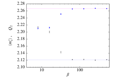
Figure 2: (Color online) Convergence test for the plaquette model at a system size $L=32$ and coupling $\alpha=1.82$ displaying the two quantities $Q_{2}$ (upper curve) and $\langle|m_{s}^{z}|\rangle$ (lower curve). Ground-state properties are sampled for $\beta\mathrel{\hbox to0.0pt{\lower 4.0pt\hbox{\hskip 1.0pt$\sim$}\hss}\raise 1.0pt\hbox{$>$}}100$. The staggered magnetization was multiplied by $25$ for convenience.

II.2 Observables

In order to determine the quantum critical point, we look at well-known observables. Next to trivial quantities such as the average energy per site $e$, we consider the staggered magnetization defined by

$$m^{z}_{\mathrm{s}}=\frac{1}{N}\sum_{i}^{N}S_{i}^{z}(-1)^{x_{i}+y_{i}}\,,$$ (3)

where the sum runs over all $N=L^{2}$ lattice sites, together with the usual Binder parameters

$$Q_{1} =\frac{\langle(m_{\mathrm{s}}^{z})^{2}\rangle}{\langle|m_{\mathrm{s}}^{z}|\rangle^{2}}\,,$$ (4)

$$Q_{2} =\frac{\langle(m_{\mathrm{s}}^{z})^{4}\rangle}{\langle(m_{\mathrm{s}}^{z})^{2}\rangle^{2}}\,.$$ (5)

These parameters are dimensionless and they possess the property to cross at the quantum critical point. Note that the staggered magnetization and the Binder parameters can be determined quite efficiently by averaging over spin representations in the operator directionSyljuåsen and Sandvik (2002) of the SSE representation. The brackets $\langle\dots\rangle$ therefore signify $\langle m_{\mathrm{s}}^{z}\rangle\equiv\langle\langle m_{\mathrm{s}}^{z}\rangle_{\mathrm{op}}\rangle_{\mathrm{conf}}$.

Second, we study the correlation length $\xi$ of the system. We employ the standard second-moment approach, which uses the structure factors $S(\mathbf{q})$ defined by

$$S(\mathbf{q})=\frac{1}{N}\sum_{i,j}\exp(-\mathrm{i}\mathbf{q}(\mathbf{r}_{i}-\mathbf{r}_{j}))\langle S^{z}_{i}S^{z}_{j}\rangle\,,$$ (6)

with $\mathbf{q}$ being a wave vector in Fourier space and $\mathbf{r}_{i}$ the vector pointing to site $i$ on the real space lattice. This quantity can be efficiently obtained for arbitrary $\mathbf{q}$ during the diagonal update, as

$$S(\mathbf{q})=\left\langle\frac{1}{Nn}\left(\sum_{p}^{n-1}m_{q}[p]m_{q}[p]^{\star}\right)\right\rangle\,,$$ (7)

where the index $p$ is running over the operator sequence having $n$ non-unit operators. The quantities $m_{q}[p]$ are defined at SSE operator slice $p$ as $m_{q}[p]=\sum_{i}^{N}S^{z}_{i}[p](\cos(\mathbf{q}\mathbf{r}_{i})-\mathrm{i}\sin(\mathbf{q}\mathbf{r}_{i}))$ and $m_{q}[p]^{\star}$ denotes its complex conjugate. The correlation length is then estimated by

$$\xi_{y}=\frac{L_{y}}{2\pi}\sqrt{\frac{S(\pi,\pi)}{S(\pi,\pi+2\pi/L_{y})}-1}\,.$$ (8)

For the anisotropic ladder model we expect $\xi_{x}\neq\xi_{y}$ on the square lattice. We found it most useful to look at the correlation length in $y$-direction of the system. This choice is arbitrary but somehow motivated from Ref. Wenzel et al., 2008a because $\xi_{y}$ showed good scaling for the staggered Heisenberg model. From standard finite-size scaling theory we expect the quantity $\xi_{y}/L$ to cross for different lattice sizes at the quantum critical point. In case of the symmetric plaquette model, an improved estimate for the spatial correlation length can be obtained by taking

$$\xi=\frac{1}{2}\left(\xi_{x}+\xi_{y}\right).$$ (9)

Lastly, we consider the spin stiffness $\rho_{s}$ given bySandvik (1997)

$$\rho_{s}=\frac{3}{4\beta}\langle w_{x}^{2}+w_{y}^{2}\rangle\,,$$ (10)

with $w_{x}$,$w_{y}$ being winding numbers defined by

$$w_{\lambda}=(N^{+}_{\lambda}-N^{-}_{\lambda})/L_{\lambda}\quad(\lambda=x,y)\,.$$ (11)

The symbols $N^{+}_{\lambda}$ and $N^{-}_{\lambda}$ represent the number of operators of type $S^{+}_{i}S^{-}_{j}$ and $S^{-}_{i}S^{+}_{j}$ along the $\lambda$-direction in the SSE configuration. The spin stiffness measures the response in free energy upon a boundary twist on the staggered magnetization (the order parameter field $\theta$) and is also called superfluid density in other contexts. At a quantum critical point in a 2D system it is expected to scale as $\rho_{\mathrm{s}}\sim L^{d-2-z}$, where $z$ is the dynamical critical exponent.Fisher et al. (1989); Wang et al. (2006)

II.3 Finite-size scaling

In this paper, we employ a variety of finite-size scaling methods to determine various critical quantities from the quantum critical point to the critical exponents. To this end, we make use of the standard scaling ansatz in the vicinity of the critical point

$$\mathcal{O}_{L}(t)=L^{\lambda/\nu}g_{\mathcal{O}}(tL^{1/\nu})\,,$$ (12)

where $\nu$ is the critical exponent of the correlation length, $\lambda$ the critical exponent of the quantity $\mathcal{O}$, $g_{\mathcal{O}}(x)$ the scaling function, $t$ the reduced coupling defined by $t=(\alpha-\alpha_{\mathrm{c}})/\alpha_{\mathrm{c}}$, and $L$ the lattice size.

Analysis to (12) was performed in the previous QMC study on the ladder model in Ref. Matsumoto et al., 2001. Here, we would like to go one step further and take leading corrections to scaling into account. Apart from higher order terms $O(1/L^{2})$, the renormalization group (RG) then predicts a scaling of the form

$$\mathcal{O}_{L}(t)=L^{\lambda/\nu}\left[g_{\mathcal{O}}(tL^{1/\nu})+L^{-\omega}g_{\omega}(tL^{1/\nu})\right]\,,$$ (13)

where $\omega$ is the leading correction exponent and $g_{\omega}(x)$ another scaling function. Writing $g_{\omega}(x)=c(x)g_{\mathcal{O}}(x)$, this becomes

$$\mathcal{O}_{L}(t)=L^{\lambda/\nu}\left(1+c(x)L^{-\omega}\right)g_{\mathcal{O}}(x)\,,$$ (14)

with $x=tL^{1/\nu}$ and a coefficient $c(x)$ depending on $x$. To zeroth order, and for $x$ small we may set $c(x)\approx c=\mathrm{const}$ and arrive at the usually employed form

$$\mathcal{O}_{L}(t)=L^{\lambda/\nu}(1+cL^{-\omega})g_{\mathcal{O}}(x)\,.$$ (15)

We consider (15) as our primary ansatz in the data analysis.

Note, that in the literature, another ansatz in form of

$$\mathcal{O}_{L}(t)=L^{\lambda/\nu}(1+cL^{-\omega})g_{\mathcal{O}}(tL^{1/\nu}+dL^{-\phi/\nu})\,,$$ (16)

has been discussed which represents an effective approximation to (13) in the vicinity of the quantum critical point.Beach et al. (2005); Wang et al. (2006) Here, $\omega$ and $\phi$ represent effective corrections, approximating the correct RG behavior. In Ref. Wang et al., 2006, which is closely related to the present paper, the authors employed (16) and obtained results in excellent agreement with the expectations. Here, we will primarily employ (15) and in some instances compare our result to (16). In any case, we use this procedure mainly to obtain the critical coupling $\alpha_{\mathrm{c}}$. We emphasize that final results of critical exponents will be given as obtained from ordinary scaling methods at the critical point ($x=0$), which are described in Sec. IV.

Data analysis according to Eq. (15) is known as “data collapsing”. In practice, this can often be achieved by Taylor expanding the scaling function $g_{\mathcal{O}}(x)$ for $x\to 0$ into a polynomial of the form

$$g_{\mathcal{O}}(x)=g_{0}+g_{1}x+g_{2}x^{2}+\dots\,.$$ (17)

Using this ansatz, relation (12) is turned into

$$\mathcal{O}_{L}(t)=L^{\lambda/\nu}\left(g_{0}+L^{1/\nu}g_{1}t+L^{2/\nu}g_{2}t^{2}+\dots\right)\,,$$ (18)

where all free parameters can then be determined by a nonlinear-fit of the measured data. The generalization to (15) is obvious.

We have recently implemented a related method, which does not need to make use of Taylor expanding the function $g_{\mathcal{O}}(x)$.Wenzel et al. (2008b) Using multihistogram techniques, it is possible to directly perform a collapse of the data by minimizing the weight function

$$\sigma_{\mathcal{O}}^{2}=\int_{x_{\mathrm{min}}}^{x_{\mathrm{max}}}\mathrm{d}x\left[\overline{\widehat{\mathcal{O}}_{L}^{2}}(x)-\overline{\widehat{\mathcal{O}}}_{L}^{2}(x)\right]\,,$$ (19)

where $\widehat{\mathcal{O}_{L}}(x)=\mathcal{O}_{L}(t)/(L^{\lambda/\nu}(1+cL^{-\omega}))$ and $x=tL^{1/\nu}$. With $\overline{\widehat{\mathcal{O}}_{L}}(x)\equiv\sum_{L}\widehat{\mathcal{O}}_{L}(x)/n_{L}$, we denote the average over $n_{L}$ lattice sizes. For the quantities $Q_{1}$, $Q_{2}$, $\xi_{y}/L$, $\xi/L$, and $\rho_{\mathrm{s}}L$ we have $\lambda/\nu=0$.

Figure 3: Behavior of different observables close to the quantum critical points. Different curves correspond to different system sizes (see Table 1), where larger slope means larger system size. The left column displays (a) the spin stiffness multiplied by the system size $L$, (b) the correlation length $\xi_{y}$ divided by system size $L$, and (c) the Binder parameter $Q_{2}$ for the ladder model. The plots (d)-(f) in the right column show the same quantities obtained for the plaquette model.

III Simulation Results and The Critical Point

We performed various simulations on the ladder and plaquette model for lattice sizes specified in Table 1 employing the methods described in the last section. All runs where done using periodic boundary conditions. The sample size of measured data is of the order of $4\times 10^{5}$ for the plaquette model and $8\times 10^{5}$ in case of the ladder model, giving an indication that the ladder model is somewhat harder to simulate. We typically performed $1\times 10^{4}$ sweeps for equilibration. Measurements were taken every sweep and each sweep constructed as many loops as necessary in order to visit $2n$ vertices in the SSE operator expansion on average.

Table 1: Summary of lattice sizes $L$ studied in the simulations.

model	lattice sizes $L$
ladder	$8,10,12,14,16,20,24,28,32,36,40,52,64$
plaquette	$8,10,12,16,20,24,28,32,36,40,44,48,56,72$

A summary of the raw data obtained from the simulations is displayed in Fig. 3, where we show the spin stiffness $\rho_{\mathrm{s}}$, the correlation length $\xi$ and the Binder parameter $Q_{2}$. The left and right panels in Fig. 3 distinguish results for the ladder and plaquette model, respectively. Evidently, all quantities cross close to an apparent quantum critical point justifying the scaling assumptions for the observables described above. However, clear finite-size corrections can be observed for both cases as the crossing points for small lattice sizes show large displacements. This behavior is expected and in accordance to the data published in Ref. Wang et al., 2006. Our hope is that those corrections can be described by the correction terms included in the scaling ansatz (15) (or (16)). Using the raw data, we will now try to extract a precise estimate of the quantum critical point. To reach this aim, we will follow a two-stage process, starting with an analysis of the crossing points followed by a finite-size scaling investigation using the collapsing technique.

This will in principle also give us estimates of critical exponents but we leave this issue for a more detailed investigation in Sec. IV using ordinary and well-established methods.

III.1 Estimation of the critical point from curve crossings

Finite-size scaling analysis with scaling functions involving many free parameters is a tedious and difficult task due to well-known problems of multidimensional nonlinear minimization. Before we attempt to perform a full finite-size scaling study using Eq. (15), we would therefore like to set bounds on the possible values of the critical coupling $\alpha_{c}$. To this end, a convenient approach consists in looking at the scaling of crossing points of curves at $L_{1}$ and $L_{2}$ (where $L_{2}=2\,L_{1}$) for different values of $L_{1}$. The crossing points are easily obtained using either the multihistogram method or fitting data at $L_{1}$ and $L_{2}$ to the simple scaling ansatz in Eq. (12) (using polynomial interpolation). Performing this procedure on the various observables of Fig. 3 (and $Q_{1}$) yields the plots of Fig. 4, which show convergence of the intersection points to the quantum critical point in the thermodynamic limit. The plots are presented with an $x$-axis as $1/L$, since we do not know the correct scaling a-priori.

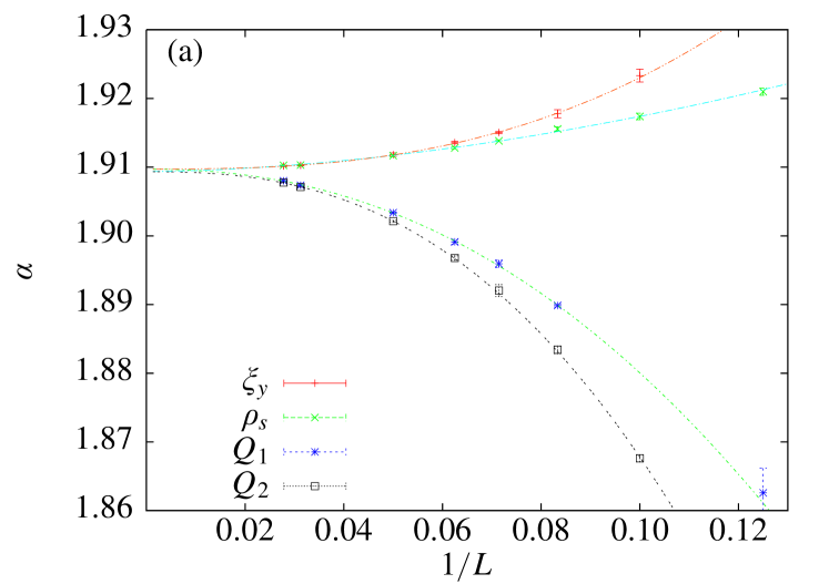
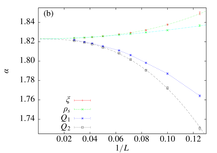
Figure 4: (Color online) Crossing points from data at $L$ and $2L$ of the four quantities $\rho_{s}L$, $\xi/L$, $Q_{1}$, and $Q_{2}$ versus the inverse lattice size. At $L=\infty$ all curves should meet and define the quantum critical point $\alpha_{c}$. (a) Analysis for the ladder model. (b) Same for the plaquette model.

The qualitative behavior of the different quantities toward the critical point is rather similar to Ref. Wang et al., 2006. We find, that for both models the spin stiffness has the least finite-size corrections, followed by the correlation length, and that the normal Binder parameter $Q_{2}$ shows large deviations at small lattice sizes. This is not necessarily a disadvantage since this often leads to better controlled fits. Before performing some fits, however, let us emphasize that in case of the staggered model considered in Ref. Wenzel et al., 2008a, the spin stiffness displayed a qualitatively different convergence toward the infinite-volume limit because there the correlation length $\xi_{y}$ showed less finite-size effects. This proves that $\rho_{\mathrm{s}}$ is not always the best quantity.

Since all quantities give a rather consistent picture in their scaling properties we can safely bracket the critical couplings from the crossings using the largest available $(L,2L)$ pair. This yields $\alpha_{\mathrm{c}}\in[1.9070,1.9105]$ and $\alpha_{\mathrm{c}}\in[1.821,1.834]$ for the ladder and plaquette cases, respectively. It is tempting to obtain a more precise estimate from fitting the crossing points to an ansatz due to BinderBinder (1981)

$$\alpha_{\mathrm{c}}(L,2L)=\alpha_{\mathrm{c}}+\frac{b}{L^{1/\nu+\omega}}\,,$$ (20)

which states that the crossings should normally converge faster than $L^{-1/\nu}$, and would indeed show no $L$-dependence at all if $\omega=\infty$, i.e. no correction. In this ansatz $b$ is a constant and we neglected subleading corrections from the “shift” term $\phi$. This term can in principle be included,Beach et al. (2005) leading to fits which are more difficult to perform. The smooth curves in Fig. 4(a) for the ladder model correspond to fits for the correlation length, the spin stiffness, and the Binder parameters $Q_{1}$ and $Q_{2}$, which yield $\alpha_{\mathrm{c}}=1.9097(3)$ ($\xi_{y}$), $\alpha_{\mathrm{c}}=1.9092(6)$ ($\rho_{\mathrm{s}}$), $\alpha_{\mathrm{c}}=1.9095(5)$ ($Q_{1}$), and $\alpha_{\mathrm{c}}=1.9093(3)$ ($Q_{2}$). They are all in agreement within error bars. For the plaquette model (Fig. 4(b)) we obtain in the same order $\alpha_{\mathrm{c}}=1.8232(3)$, $\alpha_{\mathrm{c}}=1.8228(4)$, $\alpha_{\mathrm{c}}=1.8238(8)$, and $\alpha_{\mathrm{c}}=1.8229(4)$, respectively. All fit results are summarized in Table 2, where we additionally give the fitted quantity $1/\nu+\omega$ and the quality of the fits through the chi-squared per degree of freedom ($\chi^{2}/\mathrm{d.o.f.}$). Under the assumption that the correlation length exponent $\nu\approx 0.7$, we deduce that $\omega$ lies roughly in the interval $[0.8,1.2]$ for the correlation length and the Binder parameters. For the spin stiffness, interestingly, $\omega$ seems to be smaller. The stiffness thus appears to cross close to the quantum critical point but has slow convergence towards it. On the other hand, the spin stiffness could not be well described by Eq. (20). A similar effect will, in fact, be seen in the analysis of Sec. III.2.

We feel that the critical points obtained above give a fair estimate as they agree within error bars. A posteriori, this justifies the neglection of $\phi$. Finally, it should be clear, that by the same approach other estimates, like $\nu$ and $g_{0}$, can and have been bracketed aiding in the collapse analysis now to come.

Table 2: Estimates for the critical point derived from Eq. (20) for the ladder (top group) and plaquette model (bottom group).

quantity	$\alpha_{\mathrm{c}}$	$1/\nu+\omega$	$\chi^{2}/\mathrm{d.o.f}$
$\xi_{y}$	$1.9097(3)$	$2.6(1)$	$0.85$
$\rho_{\mathrm{s}}$	$1.9092(6)$	$1.7(2)$	$1.7$
$Q_{1}$	$1.9095(5)$	$2.3(1)$	$1.2$
$Q_{2}$	$1.9093(3)$	$2.55(8)$	$0.64$
$\xi$	$1.8232(3)$	$2.6(1)$	$0.24$
$\rho_{\mathrm{s}}$	$1.8228(4)$	$1.8(1)$	$0.14$
$Q_{1}$	$1.8238(8)$	$2.2(1)$	$0.82$
$Q_{2}$	$1.8229(4)$	$2.6(1)$	$0.72$

III.2 The critical point from data collapses

In the previous section first estimates of the critical points were obtained. Next, our goal is to cross-check and possibly improve the accuracy by analyzing the data for the full set of $\alpha$ values around the crossing points including all lattice sizes in Table 1. We will therefore now elaborate on the data collapse procedure to the scaling ansatz of Eq. (15), knowing that we have to include subleading corrections terms. In this process we will leave all parameters free, since we want to avoid preoccupation about the universality class. Of course we keep in mind the bracketing of some important quantities in the previous section. Fitting is done using Eq. (17) or (19). The two approaches have been compared and we could not detect a noticeable difference in the outcome. We hence use the less time consuming approach according to Eq. (17) for which a fourth-order polynomial for $g_{\mathcal{O}}(x)$ is employed.

Due to potential problems with multidimensional fitting, the analysis is repeated for at least two different scenarios. In a first case we ignore the subleading shift correction, i.e. we set $\phi=\infty$ (or $d=0$) to obtain a first idea of the critical coupling, the correlation length exponent $\nu$ and other parameters. We will see that apart from a few exceptions, this approach actually describes our data well enough. Next we repeat the collapse taking into account possible shift corrections, described by a finite $\phi$.

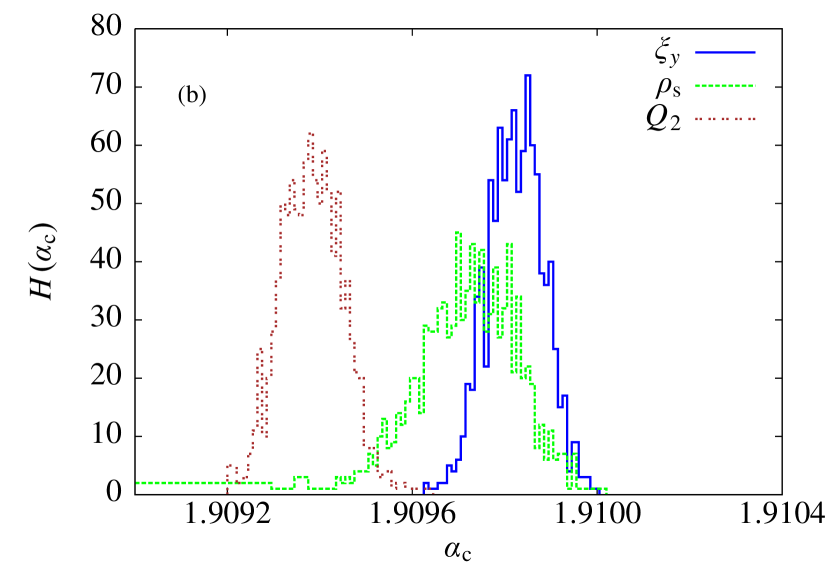
Figure 5: (Color online) (a) Visualization of the collapsing analysis. The (red) crosses ($\times$) signify the starting values and dense (blue) points ($+$) the final values of ($\alpha_{\mathrm{c}}$, $\nu$) of the procedure for the spin stiffness in case of the plaquette model. Histograms of the final value for $\alpha_{\mathrm{c}}$ for several observables for (b) the ladder model, and (c) the plaquette model.

Table 3: Tabulated results for the critical coupling ratio $\alpha_{\mathrm{c}}$, the exponent $\nu$, and the factor $g_{0}$ from the collapse procedure for both the ladder (upper group) and the plaquette model (lower group). In some cases results from two fits, with and without a $\phi$ term are given.

	restr.	$\alpha_{c}$	$\nu$	$g_{0}$
$Q_{2}$	$d=0$	$1.9094(3)$	$0.717(10)$	$2.32(1)$
$Q_{1}$	$d=0$	$1.9096(4)$	$0.72(1)$	$1.451(8)$
	no	$1.9094(3)$	$0.72(1)$	$1.449(3)$
$\rho_{\mathrm{s}}L$	no	$1.90974(15)$	$0.705(7)$	$1.155(10)$
$\xi_{y}/L$	$d=0$	$1.9098(4)$	$0.715(10)$	$0.62(1)$
$Q_{2}$	$d=0$	$1.8228(4)$	$0.716(6)$	$2.313(6)$
	no	$1.8227(4)$	$0.72(1)$	$2.311(5)$
$Q_{1}$	$d=0$	$1.8238(6)$	$0.72(1)$	$1.453(2)$
	no	$1.8228(6)$	$0.72(1)$	$1.447(4)$
$\rho_{\mathrm{s}}L$	$d=0$	$1.8230(3)$	$0.67(1)$	$1.28(3)$
	no	$1.8230(2)$	$0.707(6)$	$1.27(2)$
$\xi/L$	$d=0$	$1.8232(2)$	$0.709(6)$	$0.706(5)$
	no	$1.8231(2)$	$0.713(6)$	$0.70(1)$

All fits are repeated multiple times including random noise on the starting parameters as well as on the raw data. In the latter case, the noise is taken to be normal distributed and within the JackknifeEfron (1982) errors $\sigma$ of the original data points. We typically perform $1000$ fits for each observable. All quoted error bars are then understood as being the error bars from this bootstrapEfron (1982) procedure. Figure 5(a) outlines this procedure and shows that the collapse is well behaved. Random starting values converge to a narrow collapse region. Figures 5(b,c) display histograms of the final critical couplings obtained from the bootstrap procedure for the ladder and plaquette model, respectively. It is seen that the results are consistent as they more or less overlap, yet we note a systematic effect as the Binder parameter tends to give smaller estimates in comparison to the correlation length and the spin stiffness. This is also in accordance with the data on the full bilayer of Ref. Wang et al., 2006. Table 3 summarizes concrete results for the different models and observables. The best results for $\alpha_{\mathrm{c}}$ are obtained from the spin stiffness which usually interpolates between values from the correlation length and $Q_{2}$.

Second, we could not detect a noticeable difference in the results if we include a $\phi$ degree of freedom. An exception to this observation is the spin stiffness, which showed controlled fits only in presence of $\phi$ (which probably acts as a kind of stabilizer). This fact agrees with the observation made during the analysis of the crossing points above but is presently not well understood. The results for the exponent $\nu$ are consistent with $O(3)$ universality. Finally, typical values for $\omega$ are in the range of $\omega\in[0.8,1.3]$, consistent with the previous section. In case of the spin stiffness, we obtain $\omega\approx 1.4$ and $\phi/\nu\approx 2.5$.

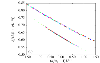
Figure 6: (Color online) Data collapses for the ladder and plaquette (wider range) model displaying (a) the Binder ratio $Q_{2}$ (where the collapse for the ladder model was shifted upwards by $0.05$ for better visibility), (b) the correlation length $\xi_{y}$ respectively $\xi$, and (c) the spin stiffness $\rho_{\mathrm{s}}$. Apart from the special case of the spin stiffness, collapses are shown without the the $\phi$ correction term.

Using these results, concrete data collapses of the original data are given in Fig. 6 which display a very good collapse quality.

In principle, one would need to perform additional investigations on the influence of size of the collapsed regime $x$ (see Eq. (19)). We have done that partly, but do not attempt a detailed extrapolation as we will extract the actual critical exponents by a different method. In any case, we believe that our estimates for $\alpha_{\mathrm{c}}$ are correct beyond doubt as they are consistently obtained from three independent methods (crossing analysis, collapse to (15), and collapse to (16)). This also justifies the use of the approximations which are present in the finite-size scaling ansatz.

We now state the main result of this section in giving our final estimates for the critical couplings. Since no details about systematic errors (e.g. from undescribed correction effects etc.) are known, a plain average of the critical coupling estimates from $Q_{2}$, $\rho_{\mathrm{s}}$, and $\xi_{y}$ is probably the best choice (and is the same as a weighted average). This way, our final estimate is $\alpha_{\mathrm{c}}=1.9096(2)$ and $\alpha_{\mathrm{c}}=1.8230(2)$ for the ladder and plaquette models, respectively. In case of the ladder model, this result is in slight disagreement with the previous value of $1.9107(2)$ in Ref. Matsumoto et al., 2001.

Before we go on, it is interesting to observe from the quantities $g_{0}$ listed in Table 3, that both the Binder parameters at the crossing point seem to be consistent within error bars among the two models, whereas the spin stiffness and the correlation length clearly do not possess this property but the reader should keep in mind that $\xi_{y}$ and $\xi$ are slightly different quantities.

IV Scaling at criticality

Having determined estimates for the critical couplings, we now turn to an investigation of the critical exponents. To this end, we make use of standard methods of Monte Carlo data analysis. Our reason to decouple this investigation from the collapse analysis is to get independent and unbiased estimates. A fit at a predetermined critical point, secondly, has less degrees of freedom and is hence easier to control.

Analysis of the exponents is performed using standard relations and definitions. An established method to obtain the correlation length exponent $\nu$, is via the slope $s_{Q_{2}}=\mathrm{d}Q_{2}/\mathrm{d\alpha}$ of the Binder parameter evaluated at the critical point. Using Eq. (13) we arrive at

$$s_{Q_{2}}\sim L^{1/\nu}\,.$$ (21)

Other exponents, in particular, $\beta$ and $\eta$ are calculated from the order parameter and the structure factor at criticality as

$$\langle|m^{z}_{s}|\rangle\sim L^{-\beta/\nu}\,,\quad S(\pi,\pi)\sim L^{1-\eta}\,,$$ (22)

where we assume Lorentz invariance, i.e., $z=1$ in $S(\pi,\pi)\sim L^{2-z-\eta}$.

In order to use Eqs. (21), (22) we need data at the quantum critical point. This can in principle be achieved by performing new simulations. Since we have rather good data in the vicinity of $\alpha_{\mathrm{c}}$ already, we instead choose to compute $s_{Q_{2}}$, $m^{z}_{s}$, and $S(\pi,\pi)$ from polynomial interpolation or multihistogram reweighting as employed in the last section. We have checked the consistency of the two approaches and use the first method from here on. Again, a bootstrap with $1000$ samples is performed on top of this interpolation, varying the raw input data within the uncertainties.

Figure 7: (Color online) Finite-size scaling using (a) the slope $s_{Q_{2}}$ of the Binder parameter, (b) the staggered magnetization, and (c) the staggered structure factor $S(\pi,\pi)$. These quantities are computed at the critical points determined in Sec. III.

Figure 7 summarizes and displays the critical data so obtained. All plots are in a $\ln-\ln$ style vs. the lattice size $L$. It is evident that straight lines represent the data rather well. To make this statement more quantitative we now perform and present detailed fits and their results in Table 4.

Table 4: Fit results for the critical exponents $\nu$, $\beta/\nu$, and $\eta$. We summarize results including a variation of the critical point within its error bar. For the ladder model (top group of values) fit results and quality of fits are also given at the previous best estimate of $\alpha_{\mathrm{c}}$. The bottom group are results for the plaquette model. Numbers in $[\ldots]$ brackets denote the $\chi^{2}/\mathrm{d.o.f}$. For comparison relevant reference values for the 3D $O(3)$ universality class are given in the last line.

$\alpha_{\mathrm{c}}$	$\nu$	$\beta/\nu$	$\eta$
$1.9096-\sigma$	$0.712(4)$ $[1.8]$	$0.516(2)$ $[0.5]$	$0.026(2)$ $[0.2]$
$1.9096$	$0.711(4)$ $[1.8]$	$0.518(2)$ $[1.1]$	$0.029(5)$ $[0.8]$
$1.9096+\sigma$	$0.710(4)$ $[1.8]$	$0.519(3)$ $[2.5]$	$0.032(7)$ $[1.4]$
$1.9107$	$0.709(3)$ $[1.7]$	$0.525(8)$ $[15.3]$	$0.051(10)$ $[12]$
$1.8230-\sigma$	$0.708(4)$ $[0.99]$	$0.515(2)$ $[0.84]$	$0.025(4)$ $[0.15]$
$1.8230$	$0.706(4)$ $[1.04]$	$0.516(2)$ $[0.40]$	$0.028(3)$ $[0.31]$
$1.8230+\sigma$	$0.706(4)$ $[1.10]$	$0.517(2)$ $[1.6]$	$0.031(5)$ $[0.80]$
Ref. Campostrini et al.,2002	$0.7112(5)$	$0.5188(3)$	$0.0375(5)$

For each quantity, 3 fits are performed corresponding to the best estimate of $\alpha_{\mathrm{c}}$, as well as its lower and upper bounds from the uncertainty. In case of the ladder model, we also try a further fit at the previous estimate of Ref. Matsumoto et al., 2001. Several observations can be made regarding our results. First, the exponent $\nu$ obtained from the slope of the Binder parameter is rather insensitive to the variation in $\alpha_{\mathrm{c}}$. Medium to good quality fits can be performed for lattice sizes $L>12$ for both models. All results for $\nu$ are consistent with the best known value $0.7112(5)$ for the 3D $O(3)$ universality class.Campostrini et al. (2002) Our estimate for $\nu$ as in Table 4 improves the accuracy compared to Ref. Matsumoto et al., 2001 by about one order of magnitude. However, we do not quite reach the level presented for the bilayer models.Wang et al. (2006) This could be related to the more complicated nature of the phase transition in planar models, where in-plane symmetries are broken.

In case of the exponent $\beta/\nu$, good fits to Eq. (22) could be performed for $L>16$ resulting in almost perfect agreement with the reference value of $\beta/\nu=0.5188(3)$, which we computed from Ref. Campostrini et al., 2002. Note that in case of the ladder model, however, the $\chi^{2}/\mathrm{d.o.f}$ increases by one order of magnitude accompanied by an increase of the value of $\beta/\nu$ when performing the fit at the previous estimate for $\alpha_{\mathrm{c}}$. This indicates that the result of this paper indeed captures the critical point in the ladder model more accurately. The same observation is true for the exponent $\eta$. All results for this exponent are quoted for lattice sizes $L>20$, indicating that this quantity is harder to estimate. Yet, our results are still consistent or close to the reference value. A natural check on the consistency of our results is a test of the (hyper)scaling relation $2\beta/\nu=(d+z-2+\eta)$, which seems to be satisfied for nearly all cases, but it is also clear that $\eta$ and $\beta$ are probably strongly correlated as they derive from almost the same quantity.

Finally, the interested reader is referred to Ref. Wenzel et al., 2008a for a slight extension of the current scaling analysis. In that reference a further comparison regarding the Binder parameter at the critical point in different planar and bilayer Heisenberg models is presented.

V Summary and Conclusions

In conclusion, we have considered two particular geometric arrangements of competing interactions in 2D planar quantum Heisenberg models complementing work we have started in Ref. Wenzel et al., 2008a. From detailed QMC simulations and a finite-size scaling study, this work provides a first high-precision value for the critical point in the plaquettized Heisenberg model and improves the value for the ladder model. In both cases, the use of correction terms and a combined analysis of different quantities is essential. For both models we derive the full set of critical exponents and improve their accuracy by about one order of magnitude (from $\nu=0.71(3)$ to $0.711(4)$) for the ladder model. These values are in excellent agreement with the classical 3D $O(3)$ universality class.Campostrini et al. (2002); Holm and Janke (1993) As outlined above, the new estimates will be useful and necessary in connection with the recent fascinating studies on impurity based questions. In this regard, an extension from bilayer to planar models has yet to be done.

Note added. Recently, a report by Albuquerque et al.Albuquerque et al. (2008) appeared, which also presents simulations on the plaquettized Heisenberg model. Since their motivation is mainly oriented towards showing the applicability of the contractor renormalization (CORE) method to quantum spin systems, less emphasis is spent on the analysis of the critical point in detail.