Spectroscopic and Photometric evidence of two stellar populations in the Galactic Globular Cluster NGC 6121 (M4)

Abstract

Aims. We present abundance analysis based on high resolution spectra of 105 isolated red giant branch (RGB) stars in the Galactic Globular Cluster NGC 6121 (M4). Our aim is to study its star population in the context of the multi-population phenomenon recently discovered to affect some Globular Clusters.

Methods. The data have been collected with FLAMES+UVES, the multi-fiber high resolution facility at the ESO/VLT@UT2 telescope. Analysis was performed under LTE approximation for the following elements: O, Na, Mg, Al, Si, Ca, Ti, Cr, Fe, Ni, Ba, and NLTE corrections were applied to those (Na, Mg) strongly affected by departure from LTE. Spectroscopic data were coupled with high-precision wide-field UBVI_C photometry from WFI@2.2m telescope and infrared JHK photometry from 2MASS.

Results. We derived an average $\rm{[Fe/H]}=-1.07\pm 0.01$ (internal error), and an $\alpha$ enhancement of $\rm{[\alpha/Fe]}=+0.39\pm 0.05$ dex (internal error). We confirm the presence of an extended Na-O anticorrelation, and find two distinct groups of stars with significantly different Na and O content. We find no evidence of a Mg-Al anticorrelation. By coupling our results with previous studies on the CN band strength, we find that the CN strong stars have higher Na and Al content and are more O depleted than the CN weak ones. The two groups of Na-rich, CN-strong and Na-poor, CN-weak stars populate two different regions along the RGB. The Na-rich group defines a narrow sequence on the red side of the RGB, while the Na-poor sample populate a bluer, more spread portion of the RGB. In the $\rm{U}$ vs. $\rm{U-B}$ color magnitude diagram the RGB spread is present from the base of the RGB to the RGB-tip. Apparently, both spectroscopic and photometric results imply the presence of two stellar populations in M4. We briefly discuss the possible origin of these populations.

1 Introduction

Observational evidence for variations in the chemical composition of light elements in Globular Cluster (GC) stars were known since Cohen (1978), who noted a scatter in Na among stars in M3 and M13. During the last few decades, high resolution spectroscopic studies have definitely confirmed that a GC stellar population is not chemically homogeneous. Even if GC stars are generally homogeneous in their Fe-peak element content, they show large star-to-star abundance variations in the light elements such as C, N, O, Na, Mg, Al, and others (see Gratton et al. 2004 for a review).

During the last twenty years, it has become clear that in red giant stars the abundances of some of these elements follow a well defined pattern. In particular, there are clear anticorrelations between the Na and O content, and between Mg and Al. Variations in the molecular CH, CN and NH band strengths, due to a spread in the abundances of carbon and nitrogen have been observed, as well as anticorrelations between CH and CN strengths, and, in some cases, a clear bimodality in the CN content.

Despite the spectroscopic observational evidence collected in more than thirty years, the pattern in the light elements is not yet well understood. Two scenarios have been proposed to explain this observed chemical heterogeneity: the evolutionary scenario and the primordial one, both apparently supported by observations.

The observed decline of C content (e.g. in M13, as shown by Smith & Briley 2006) and the decreasing ratio $\phantom{}{}^{12}\rm{C}/\phantom{}^{13}\rm{C}$ (observed in M4 and NGC 6528 by Shetrone 2003) along the RGB phase, support the evolutionary scenario. According to this theory, the origin of the observed star-to-star scatter in some elements is due to the mixing of CNO-cycle-processed material transported, in a way not well understood yet, to the stellar surface. In this way the observed anticorrelations would be present in the evolved stages of the life of stars, after the RGB bump.

At odds with this scenario, in the last few years, spectroscopic studies have revealed light element abundance variations in unevolved main sequence stars and less-evolved RGB stars, fainter than the RGB bump. The Na-O anticorrelation was found at the level of the main sequence turn-off (TO) and sub giant branch (SGB) in M13 (Cohen & Meléndez 2005), NGC 6397 and NGC 6752 (Carretta et al. 2005; Gratton et al. 2001), NGC 6838 (Ramírez & Cohen 2002) and 47 Tuc (Carretta et al. 2004). In 47 Tuc, a bimodal distribution in the CN strengths, similar to that found among RGB stars (Norris & Freeman 1979), was found also in the main sequence (MS) by Cannon et al. (1998). Moreover, Grundahl et al. (2002) have shown that in NGC 6752 the observed scatter in the Str$\rm{\ddot{o}}$mgren index $c_{1}$ is due to the abundance variations in NH bands in stars both brighter and fainter than the RGB bump. This result is consistent with a primordial scenario since theory does not predict significant mixing below the luminosity of the first dredge-up, observationally corresponding to the magnitude of the RGB bump. These observations suggest that the light element variations should be primordial, i.e. they are derived from the chemical composition of the primordial site where the GC stars have been generated, or alternatively, that a second generation of stars has been formed from a medium enriched in some elements (e.g., the self enrichment model by Ventura et al. 2001). A primordial scenario in which such GCs have experienced multiple episodes of star formation challenges the paradigm that GCs host a single stellar population, i.e. that stars of a given cluster are coeval and chemically homogeneous.

Very recently, a spectacular, and somehow unexpected confirmation that, at least in some GCs, the origin of the chemical anomalies must be primordial came from high precision photometry from Hubble Space Telescope observations. The first object challenging the paradigm of GCs hosting simple stellar populations was $\omega$ Cen. As shown by Bedin et al. (2004), the MS of $\omega$ Cen is split into two sequences. But the most exciting discovery came from the spectroscopic investigation by Piotto et al. (2005), who found that the bluest MS is more metal rich than the redder one. The only way to account for the spectroscopic and photometric properties of the two main sequences is to assume that the bluest sequence is also strongly He enhanced, to an astonishingly high Y=0.38. More recently, Villanova et al. (2007) showed that the two main sequences split in at least four sub giant branches (SGB) which must be connected in some way to the multiplicity of RGBs identified by Lee et al. (1999) and Pancino et al. (2000). The metal content of the different SGBs measured by Villanova et al. (2007) also implies a large age difference among $\omega$ Cen stellar populations, larger than 1 Gyr. The exact age dispersion depends on the assumed abundances (including the He content) of the different stellar populations, and it is still controversial (Sollima et al. 2007). Villanova et al. (2007) demonstrated that there is also a third MS, running on the red side of the two main MSs, and likely connected with the anomalous RGB-a of Pancino et al. (2000).

Omega Centauri was well-known since the seventies because of its peculiar metallicity distribution. It is the only GC showing iron-peak element dispersion (Freeman & Rodgers 1975 and, more recently, Norris et al. 1996, Suntzeff & Kraft 1996). In a sense, the findings by Pancino et al. (2000), Bedin et al. (2004), Piotto et al. (2005), Villanova et al. (2007) and Sollima et al. (2007) could simply be considered additional evidence that $\omega$ Cen is so peculiar that it might not be a GC. Perhaps, as suggested by many authors (Freeman 1993, Hughes & Wallerstein 2000), it might simply be the nucleus of a much larger system, likely disrupted by the tidal field of our Galaxy.
In this sense the most recent discovery by Piotto et al. (2007) that the MS of NGC 2808 is split into three, distinct sequences came as a sort of surprise, shaking at its foundation our understanding of GC stellar populations. NGC 2808 has been always considered a GC, with many peculiar properties regarding its metal content and its color-magnitude diagram, but a genuine, massive GC. Still, it hosts multiple stellar populations. Moreover, also in this case, in view of the negligible dispersion in iron-peak elements in NGC 2808, the only way so far available to reproduce the three MSs is to assume that there are three populations, characterized by three different helium contents, up to an (again) astonishingly high Y=0.40. Interestingly enough, D’Antona et al. (2005) already made the hypothesis of three groups of stars, with three different helium abundances in order to explain the peculiar, multi-modal Horizontal Branch (HB) of NGC 2808 (Sosin et al. 1997, Bedin et al. 2000). Piotto et al. (2007) simply found them in the form of a MS split. Piotto et al. (2007) also noticed that the different stellar populations in NGC 2808 are consistent with the spectroscopic observations by Carretta et al. (2006), who identified three groups of stars with different Oxygen abundances. The fraction of stars in the three abundance groups is in rough agreement with the fraction of stars in the three MSs.

NGC 2808 and $\omega$ Cen are, at the moment, the most extreme examples of a rather complex observational scenario. In fact, evidence of multiple populations has been found in other GCs, like NGC 1851 (Milone et al. 2008), NGC 6388 (Siegel et al. 2007, Piotto et al. 2008), and M54 (Piotto et al., in preparation) in the form of a split in the SGB. In NGC 1851 the presence of a group of RGB stars with enhanced Sr and Ba and strong CN bands, among the majority of CN-normal RGB stars (Yong & Grundahl 2008), and the presence of a bimodal HB, agrees with the hypothesis of two stellar generations inferred by the observed SGB split.

The extremely peculiar HB of NGC 6388 (Rich et al. 1997), with the presence of extremely hot HB stars (Busso et al. 2007) was already interpreted in terms of multiple, helium enhanced, population by Sweigart & Catelan (1998), and in the more detailed analysis by Caloi & D’Antona (2007).

As for M54, it has been recognized as the nucleus of the Sagittarius dwarf galaxy (Da Costa & Armandroff 1995; Bassino & Muzzio 1995; Layden & Sarajedini 2000), and it could simply represent what $\omega$ Cen was long time ago.

It is worth noting that the clusters showing multiplicities in their CMDs are among the most massive GCs of our Galaxy ($\rm{M>10^{6}M_{\odot}}$) and all of them have peculiar HBs, as well as peculiar abundances, including Na-O anticorrelations. However, we must also note that much less massive GCs, with no evidence of multiple populations identified so far, show very large star-to-star abundance variations. It is noteworthy to recognize here that the Na-O anticorrelation has been found in about 20 GCs (see Carretta et al. 2006 for the most updated list).

In summary, it is clear that GCs are not as simple systems as thought in the past. Up to now, we lack a complete explanation for the mechanisms necessary to understand the observational scenario. A systematic study of the chemical abundances of many stars in GCs is needed in order to better understand the star formation history of these objects.

In this work we present a study on the chemical abundances of the GC NGC 6121 (M4) from high resolution spectra of its RGB stars.

As far as we know, M4 shows no evidence of multiple stellar populations in its CMD, and its mass ($\rm{log{\frac{M}{M\odot}}=4.8}$, Mandushev et al. 1991) is much smaller than the mass of the clusters with the photometric peculiarities discussed above.

Chemical abundances from high resolution spectra of M4 RGB stars have been already measured by different groups of investigators: Gratton, Quarta & Ortolani 1986 (hereafter GQO86), Brown & Wallerstein 1992 (BW92), Drake et al. 1992 (D92), Ivans et al. 1999 (I99), and Smith et al. (2005). These authors have found a range of [Fe/H] between $-$1.3 dex (BW92) and $-$1.05 dex (D92). For further details, see I99 who have summarized the chemical abundances found in previous studies. A study by Norris 1981 (hereafter N81) of 45 RGB stars showed a CN bimodality in M4, e. g., stars of very similar magnitudes and colors have a bimodal distribution of CN band strengths. By analyzing 4 RGB stars, two selected from the CN-weak group and two from the CN-strong one, D92 (and then Drake et al. 1994) found differences in the Na and Al content. I99 found that O is anticorrelated with N, whereas Na and Al abundances are larger in CN-strong stars. Looking at the evolutionary states of these stars, both I99 and Smith & Briley 2005 (SB05) did not find any strong correlation between CN band strength and the position on the CMD. More recently, Smith et al. (2005), studying the fluorine abundance in seven RGB stars in M4, found a large variation in $\phantom{}{}^{19}$F, which is anticorrelated with the Na and Al abundances. In these previous studies, both the evolutionary scenario and a primordial one have been taken into account in order to explain the light element variations and the CN bimodality in M4.

In this work, we analyze high resolution spectra in order to study chemical abundances for a large sample of M4 RGB stars and compare our results with those of previous studies. In Section 2 we provide an overview of the observations and target sample. The membership criterion used to separate the probable cluster stars is described in Section 3, and the procedure to derive the chemical abundances is in Section 4. We present our results in Section 5, and discuss them in Section 6 and Section 7. Section 8 summarizes the results of this work.

Figure 1: Distribution of the UVES target stars on the $\rm{B}$ vs. $\rm{(B-I)}$ CMD corrected for differential reddening.

2 Observations and Data Reduction

Our dataset consists of UVES spectra collected in July-September 2006, within a project devoted to the detection of spectroscopic binaries in the GC M4, and to the measurement of the geometric distance of this cluster (Programs 072.D-0742 and 077.D-0182). Data are based on single 1200-1800 sec exposures obtained with FLAMES/VLT@UT2 (Pasquini et al. 2002) under photometric conditions and a typical seeing of 0.8-1.2 arcsec. The 8 fibers feeding the UVES spectrograph were centered on 115 isolated stars (no neighbours within a radius of 1.2 arcsec brighter than $\rm{V+2.5}$, where $\rm{V}$ is the magnitude of the target star) from $\sim 1$ mag below the HB to the tip of the RGB of M4, in the magnitude range $10.5<{\rm V}<14.0$.

The UVES spectrograph was used in the RED 580 setting. The spectra have a spectral coverage of $\sim$2000 Å with the central wavelength at 5800 Å. The typical signal to noise ratio is ${\rm S/N\sim 100-120}$.

Data were reduced using UVES pipelines (Ballester et al. 2000), including bias subtraction, flat-field correction, wavelength calibration, sky subtraction and spectral rectification. Stars were carefully selected from high quality photometric $\rm{UBVI_{C}}$ observations by Momany et al. (2003) obtained with the Wide Field Imager (WFI) camera at the ESO/MPI 2.2m telescope (total field of view $34\times 33\leavevmode\nobreak\ {\rm arcmin}^{2}$) coupled with infrared JHK 2MASS photometry (Skrutskie et al. 2006). Given the spatially variable interstellar reddening across the cluster (Cudworth & Rees 1990; Drake et al. 1994; Kemp et al. 1993; Lyons et al. 1995; and I99) we have corrected our CMDs for this effect (as done in Sarajedini et al. 2007). Fig. 1 shows the position of the target stars on the corrected B vs (B-I) CMD.

3 Radial velocities and membership

In the present work, radial velocities were used as the membership criterion since the cluster stars all have similar motion with respect to the observer. The radial velocities (${\rm v_{r}}$) of the stars were measured using the IRAF FXCOR task, which cross-correlates the object spectrum with a template. As a template, we used a synthetic spectrum obtained through the spectral synthesis code SPECTRUM (see http://www.phys.appstate.edu/spectrum/spectrum.html for more details), using a Kurucz model atmosphere with roughly the mean atmospheric parameters of our stars $\rm{T_{eff}=4500}$ K, $\rm{log(g)=2.0}$, $\rm{v_{t}=1.4}$ km/s, $\rm{[Fe/H]=-1.10}$. At the end, each radial velocity was corrected to the heliocentric system. We calculated a first approximation mean velocity and the r.m.s ($\sigma$) of the velocity distribution. Stars showing $\rm{v_{r}}$ out of more than $3\sigma$ from the mean value were considered probable field objects and rejected, leaving us with 105 UVES spectra of probable members. After this procedure, we obtained a new mean radial velocity of $70.6\pm 1$ km/s from all the selected spectra, which agrees well with the values in the literature (Harris 1996, Peterson et al. 1995).

4 Abundance analysis

The chemical abundances for all elements, with the exception of Oxygen, were obtained from the equivalent widths (EWs) of the spectral lines. An accurate measurement of EWs first requires a good determination of the continuum level. Our relatively metal-poor stars, combined with our high S/N spectra, allowed us to proceed in the following way. First, for each line, we selected a region of 20 Å centered on the line itself (this value is a good compromise between having enough points, i. e. a good statistic, and avoiding a too large region where the spectrum can be not flat). Then we built the histogram of the distribution of the flux where the peak is a rough estimation of the continuum. We refined this determination by fitting a parabolic curve to the peak and using the vertex as our continuum estimation. Finally, the continuum determination was revised by eye and corrected by hand if a clear discrepancy with the spectrum was found. Then, using the continuum value previously obtained, we fit a gaussian curve to each spectral line and obtained the EW from integration. We rejected lines if affected by bad continuum determination, by non-gaussian shape, if their central wavelength did not agree with that expected from our linelist, or if the lines were too broad or too narrow with respect to the mean FWHM. We verified that the gaussian shape was a good approximation for our spectral lines, so no lorenzian correction was applied. The typical error for these measurements is 3.6 mÅ, as obtained from the comparison of the EWs measured on stars having similar atmospheric parameters (see Sect. 5.1 for further details).

4.1 Initial atmospheric parameters

Initial estimates of the atmospheric parameters were derived from WFI $\rm{BVI}$ photometry. First-guess effective temperatures ($\rm{T_{eff}}$) for each star were derived from the $\rm{T_{eff}}$-color relations (Alonso et al. 1999). $\rm{(B-V)}$ and $\rm{(V-I)}$ colors were de-reddened using a reddening of ${\rm E(B-V)=0.36}$ (Harris 1996). Surface gravities ($\rm{log(g)}$) were obtained from the canonical equation:

${\rm log(g/g_{\odot})=log(M/M_{\odot})+4\cdot log(T_{eff}/T_{\odot})-log(L/L_{\odot})}$

where the mass ${\rm M/M_{\odot}}$ was derived from the spectral type (derived from T_eff) and the luminosity class of stars (in this case we have a III luminosity class) through the grid of Straizys & Kuriliene (1981). The luminosity ${\rm L/L_{\odot}}$ was obtained from the absolute magnitude ${\rm M_{V}}$, assuming an apparent distance modulus of $\rm{(m-M)_{V}=12.83}$ (Harris 1996). The bolometric correction ($\rm{BC}$) was derived by adopting the relation $\rm{BC-T_{eff}}$ from Alonso et al. (1999).
Finally, microturbolence velocity ($\rm{v_{t}}$) was obtained from the relation (Gratton et al. 1996):

${\rm v_{t}\ (km/s)=2.22-0.322\cdot log(g)}$

These atmospheric parameters are only initial guesses and are adjusted as explained in the following Section.

4.2 Chemical abundances

The Local Thermodynamic Equilibrium (LTE) program MOOG (freely distributed by C. Sneden, University of Texas at Austin) was used to determine the metal abundances.

The linelists for the chemical analysis were obtained from the VALD database (Kupka et al. 1999) and calibrated using the Solar-inverse technique. For this purpose we used the high resolution, high S/N Solar spectrum obtained at NOAO ($National\leavevmode\nobreak\ Optical\leavevmode\nobreak\ Astronomy\leavevmode\nobreak\ Observatory$, Kurucz et al. 1984). We used the model atmosphere interpolated from the Kurucz (1992) grid using the canonical atmospheric parameters for the Sun: $\rm{T_{eff}=5777}$ K, $\rm{log(g)}=4.44$, $\rm{v_{t}=0.80}$ km/s and $\rm{[Fe/H]=0.00}$.

The EWs for the reference Solar spectrum were obtained in the same way as the observed spectra, with the exception of the strongest lines, where a Voigt profile integration was used. In the calibration procedure, we adjusted the value of the line strength $\rm{log(gf)}$ of each spectral line in order to report the abundances obtained from all the lines of the same element to the mean value. The chemical abundances obtained for the Sun are reported in Tab. 1. The derived Na and Mg abundances were corrected for the effects of departures from the LTE assumption, using the prescriptions by Gratton et al. (1999).

Table 1: Measured Solar abundances ($\rm{log\epsilon(X)=log(N_{X}/N_{H})+12)}$.

Element	UVES	lines
$\rm{OI}$	8.83	1
$\rm{NaI_{NLTE}}$	6.32	4
$\rm{MgI_{NLTE}}$	7.55	3
$\rm{AlI}$	6.43	2
$\rm{SiI}$	7.61	12
$\rm{CaI}$	6.39	16
$\rm{TiI}$	4.94	33
$\rm{TiII}$	4.96	12
$\rm{CrI}$	5.67	32
$\rm{FeI}$	7.48	145
$\rm{FeII}$	7.51	14
$\rm{NiI}$	6.26	47
$\rm{BaII}$	2.45	2

With the calibrated linelist, we can obtain refined atmospheric parameters and abundances for our targets. Firstly model atmospheres were interpolated from the grid of Kurucz models by using the values of $\rm{T_{eff}}$, $\rm{log(g)}$, and $\rm{v_{t}}$ determined as explained in the previous section. Then, during the abundance analysis, $\rm{T_{eff}}$, $\rm{v_{t}}$ and $\rm{log(g)}$ were adjusted in order to remove trends in Excitation Potential (E.P.) and equivalent widths vs. abundance respectively, and to satisfy the ionization equilibrium. $\rm{T_{eff}}$ was optimized by removing any trend in the relation between abundances obtained from the FeI lines with respect to the E.P. The optimization of $\rm{log(g)}$ was done in order to satisfy the ionization equilibrium of species ionized differently: we have used FeI and FeII lines for this purpose. We changed the value of log(g) until the following relation was satisfied:

${\rm log\epsilon(FeII)_{\odot}-log\epsilon(FeI)_{\odot}=log\epsilon(FeII)_{\ast}-log\epsilon(FeI)_{\ast}}$

We optimized $\rm{v_{t}}$ by removing any trend in the relation abundance vs. EWs of the spectral lines. This iterative procedure allowed us to optimize the values of atmospheric parameters on the basis of spectral data, independent of colors. This is an important advantage for those clusters, as M4, that are projected in regions characterized by a differential reddening.
The adopted atmospheric parameters, together with the coordinates, the U,B,V,I_C, and the 2MASS J,H,K magnitudes, are listed in Tab. LABEL:Tab8. All the reported magnitudes are not corrected for differential reddening.
Having $\rm{T_{eff}}$ determinations independent of colors, we can verify whether the $\rm{T_{eff}}$-scale is affected by systematic errors. For this purpose we used the $\rm{T_{eff}}$ and $\rm{[Fe/H]}$ of our stars (see Sec. 6.1) to obtain intrinsic $\rm{B-V}$ colors from Alonso’s relations. These colors were compared with WFI photometry corrected for differential reddening. We obtained a reddening of:

$\rm E(B-V)=+0.34\pm 0.02$

This value agrees well with the $\rm{E(B-V)=0.36}$ of Harris (1996) and with I99 who find $\rm{E(B-V)=0.33\pm 0.01}$. Therefore, we conclude that our $\rm{T_{eff}}$-scale is not affected by strong systematic errors.
Finally we present a $\rm{v_{t}-log(g)}$ relation obtained from our data:

$\rm{v_{t}=-(0.254\pm 0.016)\cdot log(g)+(1.930\pm 0.035)}$

It gives a mean microturbolence velocity 0.15 km/s lower than that given by Gratton et al. (1996), but this is not a surprise because also in other papers (Preston et al. 2006) Gratton et al. (1996) was found to overestimate the microturbolence, especial in our $\rm{T_{eff}}$ regime. We underline that our formula is valid for objects in the same $\rm{T_{eff}}$-$\rm{log(g)}$ regime as out targets, i.e. cold giant stars.

4.3 The O synthesis

Instead of using the EW method, we measured the O content of our stars by spectral synthesis. This method is necessary because of the blending of the target O line at 6300 Å with other spectral lines (mainly the Ni transition at 6300.34 Å). For this purpose, we used a linelist from the VALD archive calibrated on the NOAO Solar spectrum as done before for the other elements, but in this case we changed the log(gf) parameter of our spectral lines in order to obtain a good match between our synthetic spectrum and the observed one.

With the calibrated linelist, it is possible to establish the O content of our targets. To this aim, we used the standard MOOG running option $synth$ that computes a set of trial synthetic spectra and matches these to the observed spectrum. The synthetic spectra were obtained by using the atmospheric parameters derived in the previous section. In this way, the Oxygen abundances were deduced by minimization of the observed-computed spectrum difference. An example of a spectral synthesis is plotted in Fig. 2 where the spectrum of the observed star #34240 (thick line) is compared with synthetic spectra (thin lines) computed for O abundances $\rm{[O/Fe]}$= +0.30, +0.47, and +0.60 dex. In the plotted spectral range, the observed spectrum is contaminated by two telluric features (not present in the models), but none affecting the O line.

The O line is faint, and we could measure the O content only for a sub-sample of 93 stars. In the remaining 12 spectra, the bad quality of the Oxygen line prevented us from measuring accurate O abundance.

Figure 2: Spectrum of the star #34240, compared with synthetic spectra in the region 6297-6302 Å, which includes the Oxygen line at 6300.31 Å. Synthetic spectra were computed for O abundances [O/Fe] = +0.30, +0.47, and +0.60 dex. Thick line is the observed spectrum, thin lines are the synthetic ones.

Figure 3: Box plot of the M4 giant star element abundances from UVES data. For each box the central horizontal line is the median of the data, while the upper and lower lines indicate the higher and lower 1$\sigma$ value respectively. The points represent the individual measurements.

5 Results

The wide spectral range of the UVES data allowed us to derive the chemical abundances of several elements. The mean abundances for each element are listed in Tab. 2 together with the error of the mean, the rms scatter and the number of measured stars ($\rm{N_{stars}}$). The rms scatter (hereafter $\sigma_{\rm{obs}}$) is assumed to be the $\rm{68.27th}$ percentile of the distribution of the measures of the single stars and the error of the mean is the rms divided by $\sqrt{\rm{N_{stars}-1}}$. In the last column the abundances derived by I99 were listed as a comparison.

The derived Na and Mg abundances were corrected for the effects of departures from the LTE assumption (NLTE correction) using the prescriptions by Gratton et al. (1999), as done for the Sun. In the paper all the used Na and Mg abundances are NLTE corrected, also were not explicitely indicated. The mean NLTE corrections obtained for [Na/Fe] and [Mg/Fe] are $-0.02$ dex and $+0.07$ dex, respectively. For the Fe abundance, we do not distinguish between the results obtained from I and II ionization stages, because their values are necessarily the same in the chosen method.

Chemical abundances for the single stars are listed in Tab. LABEL:Tab9. A plot of our measured abundances is shown in Fig. 3, where, for each box, the central horizontal line is the median values for the element, and the upper and lower lines indicate the 1$\sigma$ values higher and lower than the median values, respectively. The points represent individual measurements.

Table 2: The average abundances of M4 stars The results by I99 are shown for comparison in Column 5.

This work				I99
		$\sigma_{\rm{obs}}$	$\rm{N_{stars}}$
${\rm[OI/Fe]}$	$+0.39\pm 0.01$	0.09	93	$+0.25\pm 0.03$
${\rm[NaI/Fe]_{NLTE}}$	$+0.27\pm 0.02$	0.17	105	$+0.22\pm 0.05$
${\rm[MgI/Fe]_{NLTE}}$	$+0.50\pm 0.01$	0.06	105	$+0.44\pm 0.02$
${\rm[AlI/Fe]}$	$+0.54\pm 0.01$	0.11	87	$+0.64\pm 0.03$
${\rm[SiI/Fe]}$	$+0.48\pm 0.01$	0.05	105	$+0.55\pm 0.02$
${\rm[CaI/Fe]}$	$+0.28\pm 0.01$	0.04	105	$+0.26\pm 0.02$
${\rm[TiI/Fe]}$	$+0.29\pm 0.01$	0.05	105	$+0.30\pm 0.01$
${\rm[TiII/Fe]}$	$+0.35\pm 0.01$	0.06	105	$+0.30\pm 0.01$
${\rm[CrI/Fe]}$	$-0.04\pm 0.01$	0.05	105	–
${\rm[FeI/H]}$	$-1.07\pm 0.01$	0.05	105	$-1.18\pm 0.00$
${\rm[NiI/Fe]}$	$+0.02\pm 0.01$	0.03	105	$+0.05\pm 0.01$
${\rm[BaII/Fe]}$	$+0.41\pm 0.01$	0.09	103	$+0.60\pm 0.02$

5.1 Internal errors associated to the chemical abundances

The measured abundances of of every element vary from star to star as a consequence of both measurement errors and intrinsic star to star abundance variations. In this section, our final goal is to search for evidence of intrinsic abundance dispersion in each element by comparing the observed dispersion $\sigma_{\rm{obs}}$ and that produced by internal errors ($\sigma_{\rm{tot}}$). Clearly, this requires an accurate analysis of all the internal sources of measurement errors. We remark here that we are interested in star-to-star intrinsic abundance variation, i.e. we want to measure the internal intrinsic abundance spread of our sample of stars. For this reason, we are not interested in external sources of error which are systematic and do not affect relative abundances.
It must be noted that two sources of errors mainly contribute to $\sigma_{\rm{tot}}$. They are:

• the errors $\sigma_{\rm{EW}}$ due to the uncertainties in the EWs measures;

• the uncertainty $\sigma_{\rm{atm}}$ introduced by errors in the atmospheric parameters adopted to compute the chemical abundances.

In order to derive an estimate of $\sigma_{EW}$, we consider that EWs of spectral lines in stars with the same atmospherical parameters and abundances are expected to be equal; any difference in the observed EWs can be attributed to measurements errors. Hence, in order to estimate $\sigma_{\rm{EW}}$, we applied the following procedure:

• Select two stars (#33683 and #33946) from our sample characterized by exactly the same $\rm{T_{eff}}$, and $\rm{log(g)}$, $\rm{v_{t}}$, [Fe/H] within a range of 0.05;

• Compare the EWs of the iron spectral lines in these two stars and calculate the standard deviation of the distribution of the differences between the EWs divided by $\sqrt{2}$. We found a value of 3.6 mÅ that we assume to represent our estimate for the errors in the EWs. Iron lines were selected because Fe abundance has always been found to be the same for stars in GCs, with the exception of $\omega$ Cen. This means that any differences in the EW for the same couple of lines is due only to measurement errors;

• Calculate the corresponding error in abundance measurements ($\sigma_{\rm{EW}}$) by using a star (#21728) at intermediate temperature, assumed to be representative of the entire sample. To this aim, we selected two spectral lines for each element in order to cover the whole E.P. range, changed the EWs by 3.6 mÅ and calculated the corresponding mean chemical abundance variation. This number divided by $\sqrt{\rm{N_{lines}-1}}$ is our $\sigma_{\rm{EW}}$. Results are listed in Tab. 3.

A more elaborate analysis is required to determine $\sigma_{\rm{atm}}$. We followed two different approaches.

In order to better understand the method, it is important to summarize the role of the atmospheric parameters in the determination of chemical abundances. As fully described in sections 4.1, the best estimate of chemical abundances, $\rm{T_{eff}}$, $\rm{v_{t}}$ and $\rm{log(g)}$ obtained from the spectrum of a single star are those that satisfy at the same time three conditions:

• removing any trend from the straight line that best fits the abundances vs. E.P.;

• removing any trend from the straight line that best fits the abundances as a function of equivalent widths;

• satisfy the ionization equilibrium through the condition $\rm{[FeI/H]=[FeII/H]}$.

Therefore, any error in the slope of the best fitting lines and in FeI/FeII determinations produces an error on the measured abundance.

In order to derive the error in temperature we applied the following procedure. First we calculated, for each star, the errors associated with the slopes of the best least squares fit in the relations between abundance vs. E.P. The average of the errors corresponds to the typical error on the slope. Then, we selected three stars representative of the entire sample (#29545, #21728, and #34006) with high, intermediate, and low $\rm{T_{eff}}$, respectively. For each of them, we fixed the other parameters and varied the temperature until the slope of the line that best fits the relation between abundances and E.P. became equal to the respective mean error. This difference in temperature represents an estimate of the error in temperature itself. The value we found is $\rm{\Delta T_{\rm eff}=40}$ K.

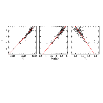
Figure 4: $\rm{I}$ magnitude (corrected for differential reddening) as a function of the atmospheric parameters for our target stars. For $\rm{T_{eff}}$ the data were fitted with a parabolic curve, for log(g) and $\rm{v_{t}}$ with a straight line.

The same procedure was applied for $\rm{v_{t}}$, but using the relation between abundance and EWs. We obtained a mean error of $\Delta\rm{v_{t}}=0.06$ km/s.

Since $\rm{log(g)}$ has been obtained by imposing the condition $\rm{[FeI/H]=[FeII/H]}$, and the measures of $\rm{[FeI/H]}$ and $\rm{[FeII/H]}$ have averaged uncertainties of $\overline{\sigma_{\rm{star}}[\rm{FeII/H}]}$ and $\overline{\sigma_{\rm{star}}[\rm{FeI/H}]}$ (where $\sigma_{\rm{star}}[\rm{Fe/H}]$ is the dispersion of the iron abundances derived by the various spectral lines in each spectrum and given by MOOG, divided by $\sqrt{\rm{N_{lines}-1}}$), in order to associate an error to the measures of gravity we have varied the gravity of the three representative stars such that the relation:

$\rm{[FeI/H]-\overline{\sigma_{star}[FeI/H]}=[FeII/H]+\overline{\sigma_{star}[FeII/H]}}$

was satisfied. The obtained mean error is $\Delta[\rm{log(g)}]$=0.12.

Once the internal errors associated to the atmospheric parameters were calculated, we re-derived the abundances of the three reference stars by using the following combination of atmospheric parameters:

• ($\rm{T_{eff}}\pm\Delta(\rm{T_{eff}})$, $\rm{log(g)}$, $\rm{v_{t}}$)

• ($\rm{T_{eff}}$, $\rm{log(g)}\pm\Delta(\rm{log(g)})$, $\rm{v_{t}}$)

• ($\rm{T_{eff}}$, $\rm{log(g)}$, $\rm{v_{t}}\pm\Delta(\rm{v_{t}})$)

where $\rm{T_{eff}}$, $\rm{log(g)}$, $\rm{v_{t}}$ are the measures determined in Section 4.2.

The resulting errors in the chemical abundances due to uncertainties in each atmospheric parameter are listed in Tab. 3 (columns 2, 3 and 4). The values of $\sigma_{\rm{atm}}$ (given by the squared sum of the uncertainties introduced by each single parameter) listed in column 5 are our final estimates of the error introduced by the uncertainties of all the atmospheric parameters on the chemical abundance measurements.

We also used a second approach to estimate $\sigma_{\rm{atm}}$ as confirmation of the first method. In order to verify our derived uncertainties related to the temperature, gravity and microturbolence, we considered that RGB stars with the same $\rm{I}$ magnitude must have the same atmospheric parameters. Hence, we started by plotting the magnitude $\rm{I}$ as a function of $\rm{T_{eff}}$, $\rm{log(g)}$ and $\rm{v_{t}}$ as shown in Fig. 4. We see in this figure that the typical internal error in our $\rm{I}$ photometry ($\sim 0.01$ mag) translates into an error in temperature of $\sim 3$ K, in $\rm{log(g)}$ of $\sim 0.005$, and in $\rm{v_{t}}$ of $\sim 0.002$ km/s, each of which is absolutely negligible. The data were fitted by a parabolic curve in the case of $\rm{T_{eff}}$, and by straight lines in the cases of $\rm{log(g)}$ and $\rm{v_{t}}$. We determined the differences between the $\rm{T_{eff}}$, log(g) and $\rm{v_{t}}$ of each star and the corresponding value on the fitting curve. Assuming the 68.27th percentile of the absolute values of these differences as an estimate of the dispersion of the points around the fitting curve, all the stars with a distance from the curve larger than $3\sigma$ were rejected (the open triangles in Fig. 4). The four probable AGB stars (filled triangles) that are evident on the $\rm{B-(B-I)}$ CMD of Fig. 1 were also rejected. With the remaining stars, the curve was refitted and the differences between the atmospheric parameters of the stars and the fit were redetermined. The 68.27th percentile of their absolute values are our estimate of the uncertainties on the atmospheric parameters.

By using this second method we obtained the uncertainties $\Delta{\rm{T_{eff}}}=$37 K, $\Delta\rm{log(g)}=$0.12 and $\Delta\rm{v_{t}}=$0.06 km/s, consistent with the ones determined with the first method.

Table 3: Sensitivity of derived UVES abundances to the atmospheric parameters and EWs. We reported the total error due to the atmospheric parameters ($\sigma_{\rm atm}$), due to the error in EW measurement ($\sigma_{\rm EW}$), the squared sum of the two ($\sigma_{\rm tot}$), and the observed dispersion ($\sigma_{\rm obs}$) for each element. The FeII observed dispersion is not reported because it is necessarily the same as FeI due to the method used in this paper to obtain atmospheric parameters.

	$\rm{\Delta T_{eff}}(K)$	$\Delta$log(g)	$\Delta\rm{v_{t}}$ (km/s)	$\sigma_{\rm{atm}}$	$\sigma_{\rm{EW}}$	$\sigma_{\rm{tot}}$	$\sigma_{\rm{obs}}$
	$+40$	$+0.12$	$+0.06$
${\rm[OI/Fe]}$	–	–	–	–	–	0.04	0.09
${\rm[NaI/Fe]}$	$+0.00$	$-0.01$	$+0.02$	0.02	0.04	0.04	0.17
${\rm[MgI/Fe]}$	$-0.01$	$-0.01$	$+0.01$	0.02	0.06	0.06	0.06
${\rm[AlI/Fe]}$	$-0.01$	$-0.02$	$+0.02$	0.03	0.06	0.07	0.11
${\rm[SiI/Fe]}$	$-0.04$	$+0.03$	$+0.02$	0.05	0.03	0.06	0.05
${\rm[CaI/Fe]}$	$+0.01$	$-0.02$	$+0.00$	0.02	0.02	0.03	0.04
${\rm[TiI/Fe]}$	$+0.04$	$-0.02$	$+0.00$	0.04	0.02	0.04	0.05
${\rm[TiII/Fe]}$	$+0.03$	$-0.01$	$-0.01$	0.03	0.05	0.06	0.06
${\rm[CrI/Fe]}$	$+0.02$	$-0.01$	$+0.00$	0.02	0.06	0.06	0.05
${\rm[FeI/H]}$	$+0.04$	$+0.00$	$-0.03$	0.05	0.01	0.05	0.05
${\rm[FeII/H]}$	$-0.03$	$+0.06$	$-0.01$	0.07	0.04	0.08	–
${\rm[NiI/Fe]}$	$-0.01$	$+0.02$	$+0.01$	0.02	0.02	0.03	0.03
${\rm[BaII/Fe]}$	$+0.05$	$-0.04$	$-0.03$	0.07	0.05	0.09	0.09

Our best estimate of the total error associated to the abundance measures is calculated as

$\rm{\sigma_{tot}=\sqrt{\sigma_{EW}^{2}+\sigma_{atm}^{2}}}$

listed in the column 7 of Tab. 3. For O $\rm{\sigma_{tot}}$ was obtained in a different way since its measure was not based on the EW method (see Section 6.4). In all the plots for the error bars associated with the measure of abundance we adopted $\sigma_{\rm tot}$.

In addition, systematic errors on abundances can be introduced by systematic errors in the scales of $\rm{T_{eff}}$, log(g), $\rm{v_{t}}$, and by deviations of the real stellar atmosphere from the model (i.e. deviations from LTE). A study of the systematic effects goes beyond the purposes of this study, where we are more interested in internal star to star variation in chemical abundances.

Comparing $\sigma_{\rm{tot}}$ with the observed dispersion $\sigma_{\rm{obs}}$ (column 8) at least for the abundance ratios ${\rm[Na/Fe]}$, ${\rm[O/Fe]}$ and $\rm{[Al/Fe]}$, we found $\sigma_{\rm{obs}}$ significantly larger than $\sigma_{\rm{tot}}$, suggesting the presence of a real spread in the content of these elements within the cluster.

6 The chemical composition of M4

In the following sections, we will discuss in detail the measured chemical abundances. In addition, we will use the abundances of C and N from the literature to extend our analysis to those elements. The errors we give here are only internal. External ones can be estimated by comparison with other works (see Tab. 2).

6.1 Iron and iron-peak elements

The weighted mean of the [Fe/H] found in the 105 cluster members is

${\rm[Fe/H]=-1.07\pm 0.01\ dex}$

The other Fe-peak elements (Ni and Cr) show roughly the Solar-scaled abundance.

The agreement between $\sigma_{\rm obs}$ and $\sigma_{\rm{tot}}$ (see Tab. 3), allows us to conclude that there is no evidence for an internal dispersion in the iron-peak element content, suggesting that this cluster is homogeneous in metallicity down to the $\sigma_{\rm{obs}}$ level.

6.2 $\alpha$ elements

The chemical abundances for the $\alpha$ elements O, Mg, Si, Ca, and Ti are listed in Tab. 2. All the $\alpha$ elements are overabundant. Ca and Ti are enhanced by $\sim$0.3 dex, while Si and Mg by $\sim$0.5 dex. The results for $\rm{[O/Fe]}$ will be discussed in detail in Section 6.4.

Previous investigators (GQO86, BW92 and I99) have also found significant overabundances for both Si and Mg. In particular, for $\rm{[Si/Fe]}$ they found values higher than 0.5 dex, slightly higher than our results, while our $\rm{[Mg/Fe]}=0.50$ lies in the middle of the literature results that range between 0.37 (BW92) and 0.68 dex (GQO86). As noted by I99, the abundances of these two elements in M4 are higher if compared to the ones found in other globular clusters showing a similar metallicity, i. e. M5 (Ivans et al. 2000). I99 suggest that the higher abundances in M4 should be primordial, e.g. due to the chemical composition of the primordial site from which the cluster formed.

For $\rm{[Ca/Fe]}$ we obtained a scatter of 0.04 dex, differing from I99, who found $\sigma$=0.11 dex (see discussion in Section $6.6$). TiI and TiII show the same abundance within $3\sigma$ (see Tab. 2), with a mean of the two different ionized species of $\rm{[Ti/Fe]}=+0.32\pm 0.04$.

The average of all the $\alpha$ elements, gives an $\alpha$ enhancement for M4 of:

${\rm[\alpha/Fe]=+0.39\pm 0.05\ dex}$

In this case the agreement between $\sigma_{\rm obs}$ and $\sigma_{\rm{tot}}$ again allows us to conclude that, down to the $\sigma_{\rm obs}$ level, there is no evidence of internal dispersion for these elements, with the exception of O, which we will discuss in Section 6.4.

6.3 Barium

As in I99 and BW92, we have found a strong overabundance of Ba. We have $\rm{[Ba/Fe]}=0.41\pm 0.01$ which is about 0.2 dex smaller than in I99. In any case, our results confirm that Ba is significantly overabundant in M4, at variance with what found by GQO86, possibly solving this important issue. As deeply discussed by I99, this high Barium content cannot be accounted for mixing processes, but must be a signature of the presence of s-process elements in the primordial material from which M4 stars formed. The excess of s-process elements provides some support to the idea that the formation of the stars we now observe in M4 happened after intermediate-mass AGB stars have polluted the environment, or that it lasted for long enough to allow intermediate-mass AGB stars to strongly pollute the lower mass forming stars. We do not find any significant dispersion in Ba content for the bulk of our target stars, though there are a few outliers worth further discussion (see below).

6.4 Na-O anticorrelation

Variations in light element abundances is common among GCs, and is also present in M4. In particular, Sodium and Oxygen have very large dispersions: we obtained $\sigma_{\rm{\rm[Na/Fe]}}$=0.17 and $\sigma_{\rm[O/Fe]}$=0.09. A large star to star scatter in Sodium and Oxygen abundance in M4 was found also in other previous studies (I99, D92).

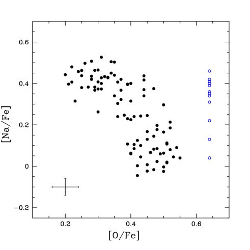
Figure 5: ${\rm[Na/Fe]}$ vs. $\rm{[O/Fe]}$ abundance ratios. The error bars represent the typical errors $\sigma_{\rm tot}$ from Tab. 3.

Figure 6: Histogram of the distribution of the ${\rm[Na/Fe]}$ abundances. The error bars represent the Poisson errors.

Sodium and Oxygen show the typical anticorrelation found in many other GCs (Gratton et al. 2004), as shown in Fig. 5, where the ${\rm[Na/Fe]}$ values are plotted as a function of ${\rm[O/Fe]}$. The open blue circles represent the 12 stars for which it was not possible to obtain a good estimate of the Oxygen abundance.

Since the Oxygen abundance was derived from just one spectral line, we adopted the following the following procedure to derive a raw estimate of the typical error $\sigma_{\rm{tot}}$ associated with each measure: we selected the group of stars with ${\rm[Na/Fe]}$$<$0.20, assuming them to be homogeneous in their O content. Under this hypothesis, the dispersion in O can be assumed to be due to the random error associated with the measured O abundance. We obtained $\sigma_{\rm[O/Fe]}=0.04$ dex, which corresponds to the error bar size in Fig. 5 and to the $\sigma_{\rm tot}$ in Tab. 3.

The only previous study showing the Na-O anticorrelation in M4 was that by I99. They analysed ${\rm[Na/Fe]}$ and ${\rm[O/Fe]}$ abundances for 24 giant stars from high resolution spectra taken at the Lick and McDonald Observatories. With respect to their work, our dispersion for [O/Fe] is quite a bit smaller (0.09 dex against their value of 0.14 dex), and our average value is larger (see Tab. 2). We have seven stars in common with their high resolution sample, and another seven with their medium resolution sample for which they derived only the Oxygen abundance. The comparison between their results and the present ones are listed in Tab. 4, where the last two columns give the differences between I99 and our results. We can note that our abundances are systematically higher than those of I99. The effect is higher for the ${\rm[O/Fe]}$, but is present for Sodium too, and could reflect the difference of $\sim$ 0.1 dex we found for the iron with respect to I99. This systematic difference does not affect the shape of the Na-O anticorrelation, but it does emphasize the overabundance of O in M4 stars with respect to other clusters with similar metallicity, as already noticed by I99: M4 stars formed in an environment particularly rich in O and possibly in Na.

The most interesting result of our investigation is that, thanks to the large number of stars in our sample, we can show that the ${\rm[Na/Fe]}$ distribution is bimodal (Fig. 6). Setting an arbitrary separation between the two peaks in Fig. 6 at $\sim$0.2 dex, we obtain, for the two groups of stars with higher and lower Na content, a mean ${\rm[Na/Fe]}=0.38\pm 0.01$ and ${\rm[Na/Fe]}=0.07\pm 0.01$, respectively.

Figure 7: Left: Distribution of stars along the Na-O anticorrelation represented by the $\rm{[O/Na]}$ ratios. Right: Distribution of the projected position P of stars on the parametric curve plotted in the inset pannel. The coordinates of the edges of the curve are indicated.

Table 4: Comparison between our ${\rm[Na/Fe]}$ and $\rm{[O/Fe]}$ and those of I99 for the stars in common. The Oxygen values were compared both with the high resolution sample of I99 ($\rm{[O/Fe]_{I99}^{(a)}}$) and with the medium resolution sample ($\rm{[O/Fe]_{I99}^{(b)}}$). The last three columns give the differences $\rm{[el/Fe]_{this\leavevmode\nobreak\ work}-[el/Fe]_{I99}}$.

ID	${\rm[OI/Fe]_{this\leavevmode\nobreak\ work}}$	$\rm{[OI/Fe]_{I99}^{(a)}}$	$\rm{[OI/Fe]_{\rm I99}^{(b)}}$	$\rm{[NaI/Fe]_{this\leavevmode\nobreak\ work}}$	$\rm{[NaI/Fe]_{I99}^{(a)}}$	$\Delta({\rm O^{(a)}})$	$\Delta({\rm O^{(b)}})$	$\Delta({\rm Na})$
L1411	$+0.28$	$+0.20$	$+0.07$	$+0.51$	$+0.43$	$+0.08$	$+0.21$	$+0.08$
L1501	$+0.34$	$+0.10$	$--$	$+0.51$	$+0.42$	$+0.24$	$--$	$+0.09$
L1514	$+0.50$	$+0.41$	$+0.41$	$+0.17$	$+0.01$	$+0.09$	$+0.09$	$+0.16$
L2519	$+0.48$	$+0.37$	$+0.37$	$+0.02$	$-0.19$	$+0.11$	$+0.11$	$+0.21$
L2617	$+0.25$	$+0.01$	$+0.07$	$+0.44$	$+0.50$	$+0.24$	$+0.18$	$-0.06$
L3612	$+0.25$	$+0.10$	$+0.12$	$+0.46$	$+0.47$	$+0.15$	$+0.13$	$-0.01$
L3624	$+0.48$	$+0.29$	$+0.27$	$+0.18$	$+0.10$	$+0.19$	$+0.21$	$+0.08$
L1403	$+0.31$	$--$	$+0.22$	$+0.53$	$--$	$--$	$+0.09$	$--$
L2410	$+0.39$	$--$	$+0.32$	$+0.11$	$--$	$--$	$+0.07$	$--$
L2608	$+0.43$	$--$	$+0.37$	$+0.24$	$--$	$--$	$+0.06$	$--$
L1617	$+0.24$	$--$	$+0.17$	$+0.46$	$--$	$--$	$+0.07$	$--$
L4415	$+0.44$	$--$	$+0.37$	$+0.37$	$--$	$--$	$+0.07$	$--$
L4421	$+0.28$	$--$	$+0.07$	$+0.44$	$--$	$--$	$+0.21$	$--$
L4413	$+0.22$	$--$	$+0.27$	$+0.48$	$--$	$--$	$-0.05$	$--$
mean	$+0.35$	$+0.21$	$+0.24$	$+0.35$	$+0.25$	$+0.16$	$+0.11$	$+0.08$

In correspondence with the two peaks in the ${\rm[Na/Fe]}$ distribution, there are also two $\rm{[O/Fe]}$ groups (Fig. 5): the first group is centered at $\rm{[O/Fe]\sim 0.30}$, while the second is at $\rm{[O/Fe]\sim 0.47}$, with a few stars having intermediate Oxygen abundance.

We have followed two methods to trace the distribution of the stars on the Na-O plane. The first method uses the ratio $\rm{[O/Na]}$ between the O and the Na abundances (Carretta et al. 2006) which appears to be the best indicator to trace the star distribution along the Na-O anticorrelation, because this ratio continues to vary even at the extreme values along the distribution. The distribution of the [O/Na] is plotted in Fig. 7 (left panel). We can identify two bulks of RGB stars in this plot: one at $\rm{[O/Na]\sim 0.40}$ and the second one at $\rm{[O/Na]\sim-0.10}$. There might be another group of stars between [O/Na]$\sim$0 and [O/Na]$\sim$0.25, but we cannot provide conclusive evidence.

Note that the two groups of stars in the Na-O anticorrelation have their corresponding peaks at $\rm{[O/Fe]\sim 0.47}$ and $\rm{[O/Fe]\sim 0.30}$, so both groups are O-enhanced.
There are no differences in $\rm{[Fe/H]}$ content between these two groups of stars: both of them have $\rm{[Fe/H]=-1.07}$ dex.

We have also analysed the distribution of stars along the Na-O anticorrelation with an alternative procedure whose steps are briefly described below:

• A parametric curve following the observed Na-O distribution as shown in the inset of the right panel of Fig. 7 has been traced;

• Each observed point in the Na-O distribution has been projected on the parametric curve;

• For each projected point, the distance (P) from the origin of the parametric curve (indicated with 0 in the inset of the right panel of Fig. 7) has been calculated;

• A histogram of the P distance distribution has been constructed.

The histogram is shown in the right panel of Fig. 7. In this case also, two peaks are evident: the first one at $\rm{P\sim 0.28}$, and the second one at $\rm{P\sim 0.58}$.

In conclusion, we obtained the Na-O anticorrelation for a large sample (93 RGB stars) in the globular cluster M4. The distribution of the objects on the Na-O anticorrelation is clearly bimodal.

6.5 Mg-Al anticorrelation

Aluminium abundances have been determined from the EWs of the AlI lines at 6696 Å and 6698 Å, and Mg abundances from the EWs of the MgI doublet at 6319 Å, 6318 Å, and of the line at 5711Å. Figure 8 shows the [Mg/Fe] as a function of [Al/Fe] and [O/Fe] (upper panels) and [Mg/Fe] and [Al/Fe] as a function of [Na/Fe] (lower panels).

In each panel the red line represents the best least squares fit to the data. The value $\rm{a}$ is the slope of the best fit straight line $\rm{y=ax+b}$. There is no clear Mg-Al anticorrelation (upper left panel of Fig. 8), although Al is more spread out than Mg ($\rm{\sigma_{[Al/Fe]}=0.11}$ vs. $\rm{\sigma_{[Mg/Fe]}=0.06}$). Both Al and Mg are overabundant, with average value of $\rm{[Al/Fe]=0.54\pm 0.01}$ and $\rm{[Mg/Fe]=0.50\pm 0.01}$ (internal errors).

The right-bottom panel of Fig. 8 shows that there is a correlation between $[\rm{Al/Fe]}$ and $\rm{[Na/Fe]}$ (higher Al abundances for higher Na content), though it is less pronounced than the Na-O anticorrelation. Aluminium spans over a range of $\sim 0.4$ dex, while Sodium covers a range of $\sim 0.6$ dex. The spread in Al content of M4 is smaller than in other clusters of similar metallicity, like M5 (Ivans et al. 1999) and M13 (Johnson et al. 2005).

Figure 9 shows that there might also be a correlation between the ${\rm[Al/Fe]}$ and ${\rm[Ba/Fe]}$.

Mg does not clearly correlate neither with Na (left-bottom panel of Fig. 8) nor O (upper-right panel of Fig. 8).

The absence of a Mg-Al anticorrelation is somehow surprising, in view of the presence of a strong double peaked Na-O anticorrelation, and of a correlation between Al and Na and possibly Al and Ba. All these correlations seems to indicate the presence of material that has gone through the s-process phenomenon. Assuming that the Na enhancement comes from the proton capture process at the expense of Ne, we can also expect that a similar process is the basis of the Al enhancement at the expense of Mg. Still, we do not find any significant dispersion in the Mg content. This problem has already been noted by I99, who suggested that the required Mg destruction is too low to be measured (see their Section 4.2.2 for further details).

Here we only add that, despite our large sample, neither in the Al nor in the Mg (and Ba) distribution can we see any evidence of the two peaks so clearly visible as in the Na and O distribution. But, in spite of the lack of a clear Mg-Al anticorreletion, we found that Na poor stars have on average higher Mg and lower Al. The difference between the median Mg and Al abundances for the Na-poor and Na-rich samples are: $\rm{[Mg/Fe]_{Na-rich}-[Mg/Fe]_{Na-poor}=-0.04\pm 0.01}$ and $\rm{[Al/Fe]_{Na-rich}-[Al/Fe]_{Na-poor}=+0.08\pm 0.02}$ This should be consistent with the scenario proposed by I99 (see their Sec. 4.2.2 for more details) who predicted that a drop of only 0.05 dex in Mg is needed to account for the observed increase in the abundance of Al. (Obviously this requires the further hypothesis that all the Na enhanced stars are also Al enhanced.)

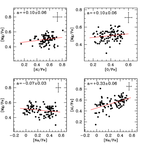
Figure 8: Bottom panels: $\rm{[Al/Fe]}$ and $\rm{[Mg/Fe]}$ abundance ratios are plotted as a function of ${\rm[Na/Fe]}$. Upper panels: $\rm{[Mg/Fe]}$ ratio as a function of $\rm{[O/Fe]}$ and $\rm{[Al/Fe]}$. In each panel the red line is the best least squares fit and $\rm{a}$ is the slope of this line. The error bars represent the typical errors $\sigma_{\rm tot}$ from Tab. 3.

Figure 9: $\rm{[Al/Fe]}$ vs. $\rm{[Ba/Fe]}$ abundance ratios. The error bars represent the typical errors $\sigma_{\rm tot}$ from Tab. 3.

6.6 CN bimodality

In this section we discuss the correlation of the $\lambda$3883 CN absorption band strength with Na, O, and Al abundances. Previous studies revealed a trend of Na and Al with the CN band strength. By studying 4 RGB stars from high resolution spectra, D92 found higher Sodium abundances in the two CN-strong stars with respect to the two CN-weak ones (Suntzeff & Smith 1991). I99 found that the Oxygen abundance is anticorrelated with Nitrogen, whereas both Na and Al are more abundant in CN-strong giants than in CN-weak ones.

In our study, two peaks in the Na distribution are evident (see Fig. 6), while there is no equally strong pattern in the Al distribution (right bottom panel of Fig. 8). The CN band strengths of red giants in M4 have been measured by N81, Suntzeff & Smith (1991), and I99. Smith & Briley 2005 (SB05) have homogenized all the available data for CN band strengths in terms of the S(3839) index, e. g. the ratio of the flux intensities of the Cyanogen band near 3839 Å and the nearby continuum. In the following, we will use the S(3839) index calculated by SB05.

In Tab. 5 the CN-index S(3839), the $\rm{[C/Fe]}$ and the $\rm{[N/Fe]}$ values (taken from SB05 and I99, respectively), and the identification as CN-strong (S), -weak (W), and -intermediate (I), are listed for our target stars with available CN data (34 stars in total). The IDs come from Lee (1977).

For these targets, Table 6 lists the mean values of the chemical abundances for CN-S and CN-W(+I) stars. The Na, O, Mg, Al and Ca abundances are from this work, the $\rm{[C/Fe]}$ values are given by SB05, while the $\rm{[N/Fe]}$ are the mean values taken from I99 for all their CN-S and CN-W stars, including stars not in common with our sample (there are only five stars in our sample with nitrogen content available). In the last column the differences $\Delta(\rm{S-W})$ between the mean values for CN-S and CN-W(+I) stars are listed.

Table 5: CN band strengths and Carbon and Nitrogen abundances for our target stars with C, N and CN measurements in the literature. We use the star identifications from Lee (1977). In the last column, S refers to CN-strong, W CN-weak and I CN-intermediate stars. The C and N abundances are from SB05 and I99, respectively.

ID	S(3839)	CN	${\rm[CI/Fe]}$	${\rm[NI/Fe]}$		ID	S(3839)	CN	${\rm[CI/Fe]}$	${\rm[NI/Fe]}$
L1411	$0.54$	S	$...$	$...$		L2626	$0.66$	S	$...$	$...$
L1403	$0.655$	S	$-0.67$	$...$		L3705	$0.20$	W	$...$	$...$
L1501	$0.61$	S	$...$	$...$		L3706	$0.16$	W	$...$	$...$
L2422	$0.69$	S	$-0.83$	$...$		L2519	$0.39$	I	$-0.50$	$+0.22$
L4404	$0.505$	S	$-0.35$	$...$		L2623	$0.245$	W	$-0.70$	$...$
L1514	$0.305$	W	$-1.12$	$+0.99$		L3721	$0.58$	S	$...$	$...$
L4415	$0.53$	S	$-0.67$	$...$		L2617	$0.63$	S	$-0.77$	$+1.05$
L4416	$0.62$	S	$-0.89$	$...$		L2711	$0.65$	S	$...$	$...$
L4509	$0.62$	S	$-0.44$	$...$		L3730	$0.24$	W	$...$	$...$
L1512	$0.61$	S	$...$	$...$		L3612	$0.65$	S	$-0.73$	$+1.02$
L1617	$0.63$	S	$-0.93$	$...$		L3621	$0.23$	W	$...$	$...$
L1619	$0.62$	S	$...$	$...$		L2608	$0.57$	S	$-0.52$	$...$
L1608	$0.60$	S	$-0.63$	$...$		L3624	$0.40$	I	$-0.67$	$+0.25$
L1605	$0.74$	S	$...$	$...$		L2410	$0.23$	W	$-0.59$	$...$
L4630	$0.505$	S	$-0.62$	$...$		L4413	$0.655$	S	$-0.32$	$...$
L3701	$0.39$	I	$...$	$...$		L4421	$0.655$	S	$-0.83$	$...$
L3404	$0.12$	W	$-0.40$	$...$		L4508	$0.14$	W	$...$	$...$

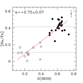
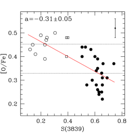
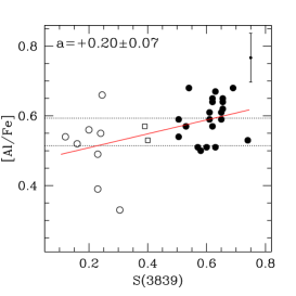
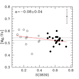
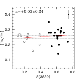
Figure 10: The abundance ratios ${\rm[Na/Fe]}$, $\rm{[O/Fe]}$, $\rm{[Al/Fe]}$, $\rm{[Mg/Fe]}$ and $\rm{[Ca/Fe]}$ are plotted as a function of the CN index S(3839). The filled circles represent the CN-S stars, the open circles the CN-W and the open squares the CN-I ones. In each panel, $\rm{a}$ is the slope of the straight line of the best least square fit. The error bars represent the typical errors $\sigma_{\rm tot}$ from Tab. 3.

Fig. 10 shows the ${\rm[Na/Fe]}$, $\rm{[Al/Fe]}$, $\rm{[O/Fe]}$, $\rm{[Mg/Fe]}$ and $\rm{[Ca/Fe]}$ values obtained in this work as a function of S(3839). In this figure CN-S objects are represented by filled circles, CN-W by open circles, and CN-I by open squares. The dotted lines represent the mean values of the abundances for the CN-S and CN-W(+I) stars; the CN-I stars were included in the CN-W group because of their similar behaviour as is clear from Fig. 10. The red lines represent the best least squares fit of the data, and $\rm{a}$ is the slope of the line. We note that the CN-S objects clearly show significantly enhanced Na abundances, while the CN-W(+I) stars have a lower Na content. The three CN-I stars show low ${\rm[Na/Fe]}$ values typical of CN-weak stars. There is also a systematic difference in Al between CN-weak and CN-strong stars, with CN-strong stars richer in Al content.

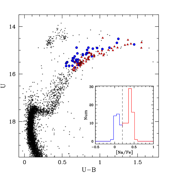
Figure 11: $\rm{U}$ vs. $\rm{(U-B)}$ CMD from WFI photometry. The distribution of the Na content for the UVES stars is shown in the inset. The stars belonging to the two different Na groups are represented in two different colors: the red triangles represent the stars with $\rm{[Na/Fe]}>0.2$ dex, and the blue circles the stars with $\rm{[Na/Fe]}\leq 0.2$ dex.

The CN-W(+I) stars have a higher O content than the CN-S as shown in the upper middle panel of Fig. 10. Fig. 10 shows some difference in $\rm{[Mg/Fe]}$ between the CN-W(+I) and the CN-S stars, with CN-W(+I) stars having slightly higher Mg abundances than the CN-S ones, but this difference is not statistically significant (see Table 6).

I99 and D92 also found that the scatter in Ca abundance correlates with the CN strength. I99 found a difference in Ca content between CN-strong and CN-weak stars by $0.08\pm 0.11$ dex. To compare, we have also analysed the Ca abundance as a function of the CN strength. In the bottom-right panel of Fig. 10, $\rm{[Ca/Fe]}$ is plotted as a function of S(3839); we can see that the difference between the two groups is 0.02 dex, smaller than what was found by I99 and not statistically significant (see Table 6).

Table 6: Mean abundance ratios and relative rms ($\sigma$) for the CN-S and CN-W(+I) groups. In the last column the difference between CN-S and CN-W(+I) stars are listed.

[el/Fe]	CN-S	$\sigma$		CN-W(+I)	$\sigma$		$\Delta({\rm S-W(+I)})$
${\rm[CI/Fe]}$	$-0.66\pm 0.05$	0.19		$-0.66\pm 0.11$	0.25		$+0.00$
${\rm[NI/Fe]}$	$+1.08\pm 0.10$	0.22		$+0.42\pm 0.19$	0.42		$+0.66$
${\rm[OI/Fe]}$	$+0.33\pm 0.01$	0.07		$+0.45\pm 0.01$	0.04		$-0.12$
${\rm[NaI/Fe]}$	$+0.41\pm 0.02$	0.07		$+0.11\pm 0.02$	0.06		$+0.30$
${\rm[AlI/Fe]}$	$+0.59\pm 0.01$	0.06		$+0.51\pm 0.03$	0.09		$+0.08$
${\rm[MgI/Fe]}$	$+0.52\pm 0.01$	0.04		$+0.54\pm 0.02$	0.06		$-0.02$
${\rm[CaI/Fe]}$	$+0.26\pm 0.01$	0.04		$+0.24\pm 0.01$	0.03		$+0.02$

7 Search for evolutionary effects

7.1 Abundances along the RGB

According to the results discussed in the previous section, we can define two groups of stars: the Na-rich stars, i. e. those with $\rm{[Na/Fe]}\geq 0.2$ and low Oxygen content which must be associated to the CN-S stars (Fig. 10), and the Na-poor stars with higher Oxygen, i. e. those with $\rm{[Na/Fe]<0.2}$, which correspond to the CN-W group. It is instructive to look at the position of the stars belonging to these two Na groups on the $\rm{U}$ vs. $\rm{(U-B)}$ CMD and on the color-color $\rm{(U-B)}$ vs. $\rm{(B-K)}$ diagram (Fig. 11 and Fig. 12, respectively). The $\rm{U}$ and $\rm{B}$ magnitudes come from our WFI photometry, the $\rm{K}$ magnitude from the 2MASS catalogue. The Na-rich stars are represented by red triangles, while the Na-poor stars by blue circles. The CMD has been corrected for differential reddening (following the same procedure used in Sarajedini et al. 2007) and proper motions. It is clear from Fig. 11 that our sample of stars mostly includes RGB stars with only three or four probable AGB stars.

Interestingly enough, the two groups of Na-rich and Na-poor stars form two distinct branches on the RGB. Na-rich stars define a narrow sequence on the red side of the RGB, while the Na-poor sample populates the blue, more spread out portion of the RGB. Even more interestingly, the anomalous broadening of the RGB is visible down to the base of the RGB, at $\rm{U}\sim 17.5$, indicating that the two abundance groups are present all over the RGB, even well below the RGB bump, where no deep mixing is expected. This evidence further strengthens the idea that the bimodal Na, O, CN distribution must have been present in the material from which the stars we presently observe in M4 originated.

Figure 11 unequivocally shows that the Na (CN) dichotomy is associated to a dichotomy in the color of the RGB stars. In order to quantify this split, we calculated for the Na-poor group of stars the mean difference in $\rm{(U-B)}$ color with respect to a fiducial line representative of the RGB Na-rich stars (see Fig. 13). The fiducial line has been obtained as follows:

• the CMD has been divided into bins of 0.30 mag in $\rm{U}$, and a median color $\rm{(U-B)}$ and $\rm{U}$ magnitude have been computed for the Na-rich ($\rm{[Na/Fe]}\geq 0.2$) stars in each bin. The median points have been fitted with a spline function which represent a first, raw fiducial line;

• for each Na-rich star, the difference in color with respect to the fiducial was calculated, and the 68.27th percentile of the absolute values of the color differences, was taken as an estimate of the color dispersion ($\sigma$). All stars with a color distance from the fiducial larger than $3\sigma$ were rejected;

• the median colors and magnitudes and the $\sigma$ of each bin were redetermined by using the remaining stars.

The leftmost panel of Fig. 13 shows the original CMD, while the rightmost one shows the CMD after subtracting from each Na-poor star the fiducial line color appropriate for its ${\rm U}$ magnitude. The differences are indicated as $\rm{\Delta(U-B)}$. We calculated the average $\rm{\Delta(U-B)}$ of Na-poor stars with $\rm{U}$$\geq$14.8. This cut in magnitude has been imposed by the poor statistics and the presence of the probable AGB stars at brighter magnitudes. The mean $\rm{\Delta(U-B)}$ value is $-0.17\pm 0.02$ (dotted line in the left most panel of Fig. 13).

The significant difference between the mean colors of the 2 groups of stars is a further evidence of the presence of two different stellar populations in the RGB of M4, to be associated with the different content of Na, and, because of the discussed correlations to different O, N, and C content.

In order to understand the origin of the photometric dichotomy, using SPECTRUM, we simulated two synthetic spectra, one representative of the Na-rich, CN-strong stars and one for the Na-poor, CN-weak ones. The two synthetic spectra were computed using as atmospheric parameters the mean values measured for the sample of our stars for which there are literature data on the CN band strengths (see Tab. 5), and assuming for the C, N, O, Na abundances the average values calculated for the CN-W(+I) and the CN-S groups and listed in Tab. 6. We then multiplied the two spectra by the efficency curve of our $\rm{U}$ and $\rm{B}$ photometric bands (Fig. 14, lower panels), and, finally, we calculated the difference between the resulting fluxes. The upper panels of Fig. 14 show the differences between the two simulated spectra as a function of the wavelength for the $\rm{U}$ (left panel) and $\rm{B}$ (right panel) panel. It is clear that the strength of the CN and NH bands strongly influences the $\rm{U}-{B}$ color. The NH band around 3360 Å, and the CN bands around 3590 Å, 3883 Å and 4215 Å are the main contributors to the effect.

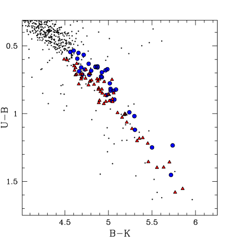
Figure 12: $\rm{(U-B)}$ vs. $\rm{(B-K)}$ diagram: $\rm{U}$ and $\rm{B}$ come from WFI photometry, $\rm{K}$ from 2MASS catalogue. The UVES stars belonging to the two different Na groups are represented as in Fig. 11.

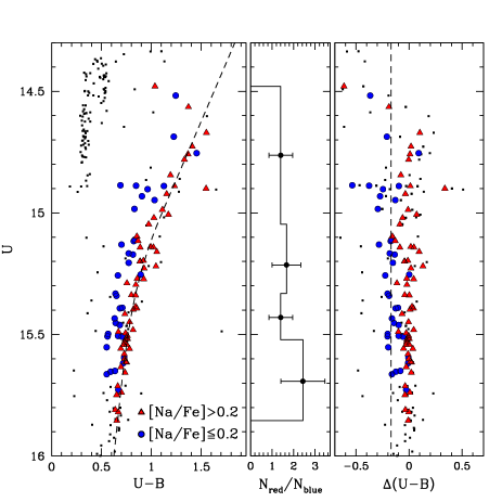
Figure 13: (Left panel) Distribution along the RGB of the stars with measured abundances. The Na-rich (red) and the Na-poor (blue) stars are represented as in Fig. 11 and Fig. 12. In the middle panel the $\rm N_{red}/N_{blue}$ ratios for the 4 selected magnitude bins are shown with their relative Poisson errors. The rightmost panel shows the color difference between each analyzed star and a reference fiducial line (dotted line).

The differences in magnitude between the CN-S and the CN-W(+I) simulated spectra in the two bands are: $\rm{\Delta(U)_{Strong-Weak}=+0.06}$ and $\rm{{\Delta(B)_{Strong-Weak}=+0.02}}$. Consequently, the expected color difference between the two groups of stars is $\rm{{\Delta(U-B)_{Strong-Weak}=+0.04}}$. This value goes in the same direction, but it is smaller than the observed one ($\rm{\Delta(U-B)_{Strong-Weak}=+0.17\pm 0.02}$). However, we note that our procedure uses simulated spectra with average abundances, and therefore should be considered a rough simulation. We cannot exclude the possibility that other effects (perhaps related to the structure and evolution of the stars with different chemical content, or effects on the stellar atmosphere associated with the complex distribution of the chemical abundances in addition to the CN band), might further contribute to the photometric dichotomy in the RGB. Surely, our simulations show that the CN-bimodality affects the $\rm{(U-B)}$ color and can be at least partly responsible for the observed spread in the $\rm U$ vs. $\rm{(U-B)}$ CMD.

Finally, we investigated whether the chemical and photometric dichotomy is related to the evolutionary status along the RGB. To this end, we have calculated the fractions of stars in the 2 Na-groups at different magnitudes along the RGB. As shown in the middle panel of Fig. 13, we divided the RGB in 4 magnitude bins containing the same number of stars with measured metal content, and calculated the ratio between the number of Na-rich ($\rm{N_{red}}$) and the number of Na-poor ($\rm{N_{blue}}$) stars in each bin. The $\rm{N_{red}/N_{blue}}$ ratios with their associated Poisson errors as a function of the magnitude are plotted the middle panel of Fig. 13. The $\rm{N_{red}/N_{blue}}$ values in the different magnitude bins are the same within the errors. A similar result is obtained if we divide the RGB in two bins only, but containing a number of stars twice as large as in the previous experiment. In this case, we have $\rm{N_{red}/N_{blue}}=1.52\pm 0.44$ for $\rm{14.0<U<14.9}$, $\rm{N_{red}/N_{blue}}=1.82\pm 0.54$ for $\rm{14.9<U<15.8}$.

Figure 15 shows the dependence of Na, Al, and S(3839) index as a function of the magnitude $\rm{U}$ (upper panel) and $\rm{B}$ (lower panel). Again, we do not see any trend of the abundances with the position of the stars along the RGB.

Figure 14: The differences (expressed in $\rm{10^{4}\ erg/cm^{2}/sec/Angstrom}$) between the CN-S and the CN-W(+I) simulated spectra in the $\rm{U}$ and $\rm{B}$ band are represented in the upper panels. The normalized response of the two filters is also shown in the lower panels.

Figure 15: Dependence of Na, Al, and S(3839) index as a function of the magnitude $\rm{U}$ (upper panels) and $\rm{B}$ (lower panels).

In conclusion, there is no evidence for a dependence of the Na content and (because of the discussed correlations) of the O, Al abundances or of the CN strength with the evolutionary status of the stars.

7.2 The RGB progeny on the HB

In the previous sections, we have identified two groups of stars with distinct Na, O, CN content, and which populate two distinct regions in the $\rm{U}$ vs. $\rm{U-B}$ CMD.

We note that Yong & Grundhal (2008), by studying 8 bright red giants in the GC NGC 1851 found a large star to star abundance variation in the Na, O, and Al content, and suggested that these abundance anomalies could be associated with the presence of the two stellar populations identified by Milone et al. (2008), a situation apparently very similar to what we have found in M4. Cassisi et al. (2008) suggest that extreme CNO variations could be the basis of the SGB split found in NGC 1851. As discussed in Milone et al. (2008) there is some evidence of a split of the RGB in NGC 1851 similar to what we have found in this paper for M4. We have investigated all available HST data of M4, including CMDs from very high precision photometry based on ACS/HST images; we could find no evidence for a SGB split (as in NGC 1851) or evidence for a MS split (as in NGC 2808 or $\omega$ Cen).

It is also useful to investigate where the progeny of the two RGB populations is along the HB. Milone et al. (2008) suggest that the bimodal HB of NGC 1851 can be interpreted in terms of the presence of two distinct stellar populations in this cluster, and tentatively link the bright SGB to the red HB (RHB) and the fainter SGB to the blue HB (BHB). M4 also has a bimodal HB, well populated on both the red and blue side of the RR Lyrae gap. Could the HB morphology of M4 be related to the CN bimodality? N81, studying the CN band strengths on a sample of 45 giant stars in M4, suggested the possibility of a relation between the HB morphology and the CN-bimodality.

To test the possible relation between the chemical and consequent RGB bimodality of M4 and the morphology of its HB, we used the WFI@2.2m instrumental photometry by Anderson et al. 2006 (Fig. 16) corrected for differential reddening, and selected the cluster members using the measured proper motions. We remark here the fact that this photometry is not the one we use in the whole paper. The homogenization between the two photometries is a difficult and long process (mainly because the fact that the $\rm{B}$ filters for the two datasets are different) beyond the scope of this work.

In our test, we used the $\rm{V}$ vs. $\rm{(B-V)}$ CMD, as in this photometric plane the two components of the HB are more clearly distinguishable.

In Fig. 16, different symbols show the red and blue HB stars that we selected. The ratio between the number ($\rm N_{BHB}$) of the HB stars bluer than the RR-Lyrae instability strip (BHB), and the total HB stars ($\rm N_{TOT}$) is:

${\rm N_{BHB}/N_{TOT}=0.56\pm 0.10}$

while the ratio between the Na rich stars (${\rm N_{NaR}}$) and the total number of stars in our spectroscopic sample (${\rm N_{S}}$) is:

${\rm N_{NaR}/N_{S}=0.64\pm 0.10}$

where the associated uncertainties are the Poisson errors. Within the statistical uncertainties, accounting for the different evolutionary times along the HB, we can tentatively associate the Na-rich stars with the BHB, and the Na-poor stars with the RHB. A direct measurement of the metal content of the HB stars is needed in order to support this suggestion..

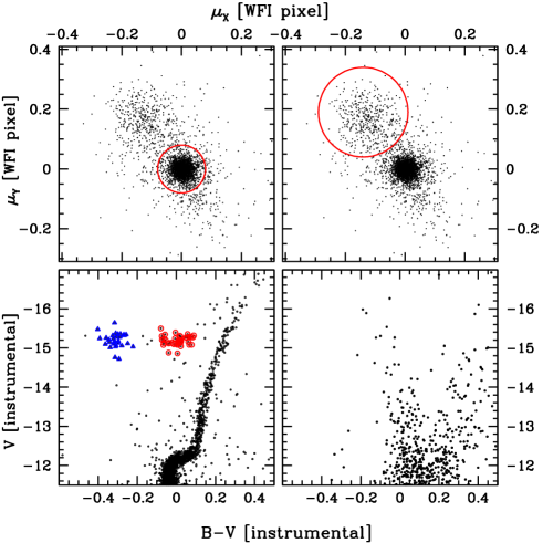
Figure 16: In the top panels, the proper motions diagrams show the separation of the probable cluster stars (left panel) from the field (right panel). In the bottom panels, the cluster and field CMD ($\rm{V}$ vs. $\rm{B-V}$) are shown for the stars within the red circle in their respective upper panels. In the M4 CMD, the stars on the red and on the blue side of the RR Lyrae instability strip are represented with red and blue symbols respectively. For this figure, the photometry, which is not photometrically calibrated, is taken from Anderson et al. (2006).

Table 7: Mean abundance ratios and relative rms ($\sigma$) for the Na-rich and Na-poor groups. In the last column, the difference between Na-rich and Na-poor stars are listed.

[el/Fe]	Na-rich	$\sigma$		Na-poor	$\sigma$		$\Delta({\rm Na_{rich-poor}})$
${\rm[OI/Fe]}$	$+0.34\pm 0.01$	0.08		$+0.47\pm 0.01$	0.04		$-0.13\pm 0.01$
${\rm[NaI/Fe]}$	$+0.38\pm 0.01$	0.08		$+0.07\pm 0.01$	0.06		$+0.31\pm 0.01$
${\rm[MgI/Fe]}$	$+0.48\pm 0.01$	0.06		$+0.52\pm 0.01$	0.05		$-0.04\pm 0.01$
${\rm[AlI/Fe]}$	$+0.57\pm 0.01$	0.08		$+0.49\pm 0.02$	0.13		$+0.08\pm 0.02$
${\rm[SiI/Fe]}$	$+0.49\pm 0.01$	0.04		$+0.46\pm 0.01$	0.06		$+0.03\pm 0.01$
${\rm[CaI/Fe]}$	$+0.28\pm 0.01$	0.04		$+0.28\pm 0.01$	0.04		$+0.00\pm 0.01$
${\rm[TiI/Fe]}$	$+0.29\pm 0.01$	0.03		$+0.29\pm 0.01$	0.05		$+0.00\pm 0.01$
${\rm[TiII/Fe]}$	$+0.35\pm 0.01$	0.07		$+0.34\pm 0.01$	0.05		$+0.01\pm 0.01$
${\rm[CrI/Fe]}$	$-0.04\pm 0.01$	0.05		$-0.03\pm 0.01$	0.05		$-0.01\pm 0.01$
${\rm[FeI/H]}$	$-1.07\pm 0.01$	0.05		$-1.07\pm 0.01$	0.05		$+0.00\pm 0.01$
${\rm[NiI/Fe]}$	$+0.02\pm 0.01$	0.03		$+0.01\pm 0.01$	0.03		$+0.01\pm 0.01$
${\rm[BaII/Fe]}$	$+0.42\pm 0.01$	0.07		$+0.40\pm 0.02$	0.13		$+0.02\pm 0.02$

8 Conclusions

We have presented high resolution spectroscopic analysis of 105 RGB stars in the GC M4 from UVES data.

We have found that M4 has an iron content $\rm{[Fe/H]=-1.07\pm 0.01}$ (the associated error here is the internal error only), and an $\alpha$ element overabundance $\rm{[\alpha/Fe]=+0.39\pm 0.05}$. Si and Mg are more overabundant than the other $\alpha$ elements, suggesting a primordial overabundance for these elements. Moreover, we also find a slight overabundance of Al. The ${\rm[Na/Fe]}$ versus [O/Fe] ratios follow the well-known Na-O anticorrelation, signature of proton capture reactions at high temperature. No Mg-Al anticorrelation was found.

We find a strong dichotomy in Na abundance, and show that it must be associated to a CN bimodality. Tab. 7 synthesizes the spectroscopic and photometric differences we found for the two groups of stars. Comparing our results to those in the literature on the CN band strength, the CN-strong stars appear to have higher content in Na and Al, and lower O than the CN-weak ones. Apparently, M4 hosts two different stellar populations. This fact is evident from a chemical abundance distribution, and is also confirmed by photometry. In fact, an inspection of the $\rm{U}$ vs. $\rm{(U-B)}$ CMD reveals a broadened RGB, and, as shown in our investigation, the two Na groups of stars occupy different positions (have different colors) along the RGB. Our sample of stars is composed of objects with $\rm{U}$ brighter than $\sim$16, but, as shown in Fig. 11, the RGB appears to be similarly spread from the level of the SGB to the RGB tip. Since our photometry has been corrected for differential reddening, we conclude that the observed RGB spread at fainter magnitudes must also be due to the metal content dichotomy.

We did not find any evident dependence of the chemical abundance distribution on the evolutionary status (along the RGB) of the target stars, from below the RGB bump to the RGB tip. This is an additional indication that the abundance spread must be primordial.

The two groups of stars we have identified both spectroscopically and photometrically seem to be due to the presence of two distinct populations of stars. The abundance anomalies are very likely due to primordial variations in the chemical content of the material from which M4 stars formed, and not to different evolutionary paths of the present stellar population of M4. This is somehow surprising, because of the relatively small mass of M4 – it is an order of magnitude smaller than the mass of $\omega$ Cen, NGC 2808, NGC 1851, NGC 6388, the other clusters in which a multiple stellar generation has been confirmed. Where did the gas which polluted the material for the CN-Na rich stars come from? Has it been ejected from a first generation of stars? How could it stay within the shallow gravitational potential of M4?

The idea that M4 hosts two generations of stars makes the multipopulation phenomenon in GCs even more puzzling than originally thought. It becomes harder and harder to accept the idea that the phenomenon can be totally internal to the cluster, unless this object is what remains of a much larger system (a larger GC or the nucleus of a dwarf galaxy?). Surely, Because its orbit involves frequent passages at high inclination through the Galactic disk, always at distances from the Galactic center smaller than 5 kpc (see Dinescu et al. 1999), M4 must have been strongly affected by tidal shocks, and therefore it might have been much more massive in the past.

Table 8: Coordinates, atmospheric parameters, U,B,V,I_C, and 2MASS J,H,K magnitudes for the analised stars. All magnitudes are not corrected for differential reddening.

ID	RA(0)	DEC(0)	Teff (K)	log(g)	vt (km/s)	U	B	V	IC	J	H	K
19925	245.81007350	-26.60153694	4050	1.20	1.67	14.83	12.76	11.04	8.97	7.59	6.63	6.38
20766	245.80811060	-26.55680649	4400	1.80	1.45	14.89	13.53	12.10	10.33	9.07	8.24	8.07
21191	245.81900040	-26.53602484	4270	1.60	1.60	14.79	13.21	11.70	9.85	8.50	7.67	7.45
21728	245.81082240	-26.51303931	4525	2.00	1.42	15.05	13.86	12.51	10.78	9.50	8.75	8.51
22089	245.82041320	-26.49663964	4700	2.28	1.36	15.28	14.36	13.14	11.54	10.34	9.61	9.47
24590	245.91667710	-26.65088182	4850	2.66	1.35	16.89	14.67	13.44	11.88	10.79	10.11	9.94
25709	245.92048770	-26.62319472	4680	2.20	1.38	15.11	14.24	12.96	11.31	10.16	9.45	9.28
26471	245.88130650	-26.60513670	4800	2.40	1.28	15.38	14.70	13.49	11.87	10.73	10.05	9.90
26794	245.90940720	-26.59866016	4800	2.45	1.44	15.69	14.94	13.71	12.08	10.92	10.25	10.07
27448	245.95330690	-26.58586889	4310	1.57	1.58	-	13.24	11.73	9.86	8.57	7.71	7.53
28103	245.84921830	-26.57493123	3860	0.50	1.62	14.75	12.52	10.71	8.51	7.01	6.03	5.75
28356	245.97324550	-26.57086633	4600	2.22	1.53	14.93	13.92	12.57	10.87	9.67	8.92	8.72
28707	245.93837450	-26.56579907	4880	2.74	1.31	15.59	14.84	13.61	11.99	10.80	10.14	9.95
28797	245.97434580	-26.56458317	4640	2.35	1.36	15.13	14.22	12.93	11.30	10.12	9.43	9.21
28847	245.90471930	-26.56390736	4780	2.40	1.27	15.43	14.76	13.54	11.88	10.67	9.98	9.77
28977	245.94551720	-26.56218478	4680	2.33	1.40	15.22	14.31	13.02	11.36	10.14	9.44	9.26
29027	245.84810750	-26.56146317	4720	2.40	1.41	15.18	14.40	13.16	11.48	10.29	9.58	9.39
29065	245.94135950	-26.56081120	4650	2.10	1.41	15.08	14.27	12.98	11.31	10.10	9.42	9.24
29171	245.89969150	-26.55958664	4880	2.64	1.26	15.72	14.95	13.73	12.09	10.88	10.16	10.00
29222	245.84606690	-26.55896241	4720	2.50	1.36	15.28	14.42	13.17	11.52	10.32	9.59	9.41
29272	245.86286750	-26.55825152	4780	2.50	1.26	15.32	14.64	13.42	11.76	10.54	9.86	9.67
29282	245.85544600	-26.55811142	4650	2.30	1.42	15.17	14.17	12.88	11.18	9.91	9.20	8.98
29397	245.87588880	-26.55671383	4600	1.50	1.78	14.60	13.53	12.20	10.47	9.25	8.54	8.32
29545	245.92749790	-26.55485385	4880	2.61	1.18	15.53	14.96	13.79	12.23	11.08	10.43	10.24
29598	245.88908940	-26.55414514	4840	2.50	1.40	15.65	14.89	13.68	12.05	10.86	10.19	10.01
29693	245.88094110	-26.55307864	4360	1.10	1.88	14.67	13.27	11.80	9.96	8.63	7.79	7.64
29848	245.89219050	-26.55108648	4780	2.52	1.24	15.48	14.75	13.52	11.87	10.69	10.00	9.83
30209	245.89243520	-26.54681482	4880	2.62	1.32	15.52	14.87	13.66	12.05	10.84	10.15	9.99
30345	245.94994400	-26.54524113	4850	2.73	1.31	15.64	15.00	13.84	12.31	11.19	10.55	10.39
30450	245.86144840	-26.54411333	4760	2.53	1.35	15.44	14.59	13.34	11.69	10.47	9.78	9.59
30452	245.88768830	-26.54411091	4830	2.56	1.25	15.72	15.07	13.88	12.26	11.07	10.38	10.22
30549	245.88815200	-26.54294543	4830	2.52	1.28	15.52	14.86	13.66	12.05	10.76	10.13	9.99
30598	245.89661740	-26.54235225	4360	1.75	1.47	14.72	13.49	12.05	10.23	8.83	8.03	7.75
30653	245.88793300	-26.54184062	4660	2.30	1.25	15.23	14.40	13.14	11.50	10.29	9.56	9.38
30675	245.90236690	-26.54157800	4830	2.58	1.35	15.52	14.77	13.58	12.00	-	-	-
30711	245.85156170	-26.54123206	4560	2.25	1.46	15.04	13.86	12.49	10.73	9.44	8.66	8.46
30719	245.90310860	-26.54116153	4810	2.65	1.24	15.79	15.13	13.97	12.43	-	-	-
30751	245.94302430	-26.54089574	4430	1.78	1.47	14.83	13.61	12.20	10.45	9.19	8.36	8.16
30924	245.89624320	-26.53883396	4810	2.60	1.28	15.48	14.79	13.61	12.03	9.55	8.81	8.40
30933	245.95895830	-26.53873652	4800	2.63	1.30	15.46	14.70	13.49	11.92	10.77	10.12	9.91
31015	245.89710880	-26.53795346	4800	2.47	1.37	14.91	14.21	13.00	11.38	10.17	9.48	9.29
31306	245.92607560	-26.53505913	4900	2.87	1.33	15.79	15.12	13.97	12.44	11.32	10.64	10.50
31376	245.91219110	-26.53432365	4800	2.59	1.36	15.37	14.52	13.29	11.68	10.46	9.79	9.59
31532	245.89561610	-26.53290071	4770	2.60	1.21	15.28	14.53	13.33	11.76	10.54	9.85	9.72
31665	245.93007130	-26.53164468	4650	2.17	1.34	14.94	14.12	12.85	11.18	9.96	9.25	9.04
31803	245.90925770	-26.53023616	4850	2.60	1.34	15.77	15.14	13.99	12.46	11.31	10.64	10.51
31845	245.85370350	-26.52982260	4700	2.42	1.31	15.23	14.34	13.09	11.44	10.16	9.49	9.29
32055	245.91709840	-26.52773869	4300	1.57	1.52	14.71	13.36	11.88	10.06	8.71	7.90	7.66
32121	245.83812920	-26.52713080	4840	2.58	1.33	15.49	14.67	13.45	11.84	10.64	9.93	9.75
32151	245.83708630	-26.52688433	4770	2.43	1.38	15.41	14.59	13.38	11.75	10.54	9.84	9.70
32317	245.86225000	-26.52536111	4510	1.88	1.43	15.06	13.93	12.56	-	9.51	8.76	8.57
32347	245.92079170	-26.52505556	4640	2.22	1.38	-	-	-	-	9.92	9.20	9.00
32583	245.89985980	-26.52267062	4850	2.54	1.34	15.46	14.80	13.61	12.03	10.80	10.16	9.95
32627	245.97840770	-26.52219757	4750	2.42	1.30	15.01	14.34	13.14	11.59	10.48	9.79	9.61
32700	245.91714040	-26.52145861	4560	2.12	1.36	14.88	13.86	12.52	10.80	9.54	8.81	8.57
32724	245.92395710	-26.52127838	4850	2.73	1.30	15.53	14.82	13.62	12.04	10.88	10.20	10.04
32782	245.89106390	-26.52065353	4880	2.60	1.24	15.81	15.10	13.94	12.38	-	-	-
32871	245.85272450	-26.51984366	4770	2.48	1.24	15.65	14.92	13.72	12.09	10.88	10.22	10.01
32874	245.91452240	-26.51985129	4600	2.04	1.38	14.82	13.99	12.72	11.07	9.86	9.13	8.93
32933	245.83915100	-26.51926550	4430	1.42	1.78	14.54	13.29	11.87	10.08	8.81	8.02	7.79
32968	245.89176500	-26.51884367	4630	2.17	1.30	15.06	14.21	12.96	11.32	10.07	9.41	9.15
32988	245.90955560	-26.51865553	4850	2.63	1.22	15.43	14.88	13.75	12.22	11.08	10.40	10.22
33069	245.94851290	-26.51783666	4940	3.05	1.36	15.45	14.71	13.53	11.99	10.86	10.19	10.02
33195	245.86426280	-26.51654913	4620	2.38	1.26	15.30	14.39	13.12	11.45	10.23	9.50	9.36
33414	245.84207930	-26.51444711	4840	2.51	1.28	15.51	14.84	13.67	12.08	10.90	10.21	10.09
33617	245.86252960	-26.51233938	4720	2.35	1.26	15.38	14.57	13.36	11.76	10.59	9.86	9.68
33629	245.83816250	-26.51221901	4930	2.80	1.33	15.77	15.06	13.90	12.34	11.17	10.48	10.36
33683	245.89914420	-26.51176320	4800	2.57	1.18	15.29	14.66	13.48	11.91	10.78	10.09	9.89
33788	245.91070220	-26.51060047	4700	2.37	1.33	15.15	14.24	12.99	11.38	10.16	9.44	9.27
33900	245.84591550	-26.50933155	4770	2.48	1.27	15.48	14.69	13.51	11.93	10.67	10.03	9.92
33946	245.84147130	-26.50887807	4800	2.62	1.15	15.63	14.89	13.71	12.14	10.95	10.29	10.15
34006	245.87135820	-26.50826984	4320	1.67	1.61	14.92	13.37	11.87	9.97	8.59	7.81	7.51
34130	245.88104790	-26.50687941	4550	2.08	1.40	14.98	13.87	12.54	10.82	9.58	8.80	8.60
34167	245.90419020	-26.50638230	4950	2.60	1.40	15.63	15.08	13.95	12.44	11.31	10.67	10.52
34240	245.90241860	-26.50557893	4470	1.95	1.41	14.86	13.74	12.37	10.63	9.35	8.62	8.43
34502	245.92046770	-26.50260567	4860	2.70	1.33	15.49	14.78	13.62	12.09	10.96	10.26	10.15
34579	245.93359340	-26.50170174	4330	1.59	1.49	14.67	13.27	11.83	10.07	8.77	7.91	7.71
34726	245.85009660	-26.50013473	4600	2.24	1.35	15.17	14.14	12.86	11.16	9.89	9.13	8.99
35022	245.94949140	-26.49673818	4850	2.51	1.36	15.50	14.79	13.62	12.10	10.96	10.31	10.11
35061	245.92398380	-26.49632071	4860	2.67	1.23	15.68	15.02	13.85	12.31	11.15	10.48	10.34
35455	245.92832620	-26.49099726	4600	2.10	1.29	14.89	13.99	12.71	11.05	9.83	9.08	8.92
35487	245.95940170	-26.49051723	4850	2.67	1.24	15.33	14.61	13.45	11.95	10.82	10.18	9.99
35508	245.85414850	-26.49026951	4780	2.48	1.18	15.66	14.96	13.80	12.23	11.05	10.37	10.18
35571	245.88484770	-26.48951670	4880	2.79	1.10	15.66	15.07	13.93	12.39	11.25	10.61	10.42
35627	245.95411440	-26.48867681	4830	2.37	1.20	15.48	14.94	13.80	12.30	11.14	10.50	10.34
35688	245.91086870	-26.48777246	4720	2.25	1.33	15.32	14.48	13.27	11.68	10.46	9.75	9.57
35774	245.87296550	-26.48657771	4450	1.92	1.44	14.88	13.68	12.32	10.59	9.32	8.57	8.35
36215	245.91658540	-26.48028356	4300	1.59	1.53	14.74	13.29	11.80	9.96	8.61	7.82	7.57
36356	245.90812220	-26.47815339	4820	2.66	1.26	15.52	14.76	13.57	12.01	10.82	10.17	9.97
36929	245.92953710	-26.46873630	4820	2.55	1.28	15.50	14.75	13.59	12.07	10.93	10.25	10.07
36942	245.97083610	-26.46848900	4800	2.66	1.23	15.43	14.74	13.56	12.04	10.90	10.23	10.08
37215	245.89085360	-26.46381984	4790	2.50	1.21	15.61	14.90	13.72	12.15	10.94	10.26	10.11
38075	245.84038430	-26.44634617	4800	2.54	1.25	15.61	14.83	13.65	12.05	10.82	10.18	9.99
38383	245.84437580	-26.43947709	4590	1.87	1.45	15.02	14.03	12.74	11.02	9.74	8.99	8.79
38399	245.88487200	-26.43904923	4730	2.35	1.38	15.23	14.37	13.14	11.51	10.29	9.56	9.39
38896	245.91189860	-26.42854610	4760	2.53	1.31	15.26	14.36	13.14	11.55	10.33	9.64	9.46
42490	246.00378460	-26.59808973	4570	2.08	1.41	14.95	13.94	12.56	10.84	9.71	8.95	8.76
42620	245.99313500	-26.59417329	4600	2.05	1.37	14.84	13.91	12.59	10.94	9.85	9.11	8.97
43370	246.03196790	-26.57365632	4920	2.80	1.32	15.63	15.03	13.85	12.31	11.29	10.66	10.50
44243	246.02382800	-26.55029031	4860	2.80	1.17	15.51	14.91	13.75	12.24	11.23	10.59	10.42
44595	246.06621120	-26.54096589	4750	2.40	1.40	15.02	14.23	13.00	11.45	10.42	9.75	9.58
44616	245.98944100	-26.54022147	4620	2.20	1.44	14.99	13.99	12.65	10.99	9.82	9.11	8.89
45163	246.00502890	-26.52572879	4770	2.40	1.26	15.27	14.59	13.40	11.88	10.81	10.17	9.98
45895	246.01787760	-26.50775258	4720	2.25	1.34	14.93	14.22	12.99	11.43	10.38	9.71	9.52
5359	245.91226500	-26.36929347	4800	2.44	1.28	15.60	14.78	13.58	12.01	10.87	10.21	10.05

Table 8: continued.

Table 9: Chemical abundances of the analised stars.

ID	[FeI/H]	[OI/Fe]	[NaI/Fe]NLTE	[MgI/Fe]NLTE	[AlI/Fe]	[SiI/Fe]	[CaI/Fe]	[TiI/Fe]	[TiII/Fe]	[CrI/Fe]	[NiI/Fe]	[BaII/Fe]
19925	$-$1.02	0.28	0.51	0.43	0.68	0.50	0.19	0.48	0.29	$-$0.04	0.09	0.64
20766	$-$1.05	0.31	0.53	0.49	0.62	0.49	0.26	0.31	0.39	$-$0.01	0.04	0.45
21191	$-$1.06	0.34	0.51	0.55	0.59	0.54	0.24	0.31	0.32	$-$0.00	0.03	0.53
21728	$-$1.06	0.31	0.37	0.52	0.68	0.47	0.28	0.32	0.30	$-$0.04	0.03	0.48
22089	$-$1.06	0.35	0.50	0.30	–	0.53	0.31	0.25	0.32	$-$0.15	0.03	0.46
24590	$-$1.07	0.50	0.30	0.61	–	0.50	0.27	0.29	0.31	$-$0.09	0.04	0.33
25709	$-$1.13	0.44	0.34	0.54	0.59	0.53	0.35	0.26	0.33	$-$0.02	$-$0.01	0.35
26471	$-$1.10	0.41	0.09	0.59	0.58	0.45	0.30	0.23	0.31	0.00	$-$0.01	0.28
26794	$-$1.17	–	0.36	0.53	–	0.50	0.34	0.34	0.39	$-$0.01	0.03	0.33
27448	$-$1.12	0.51	0.11	0.50	0.42	0.45	0.29	0.39	0.36	$-$0.02	0.03	0.35
28103	$-$1.08	0.50	0.17	0.41	0.33	0.55	0.16	0.48	0.26	$-$0.11	0.01	0.26
28356	$-$1.14	0.44	0.37	0.55	0.57	0.53	0.28	0.29	0.37	0.04	0.05	0.39
28707	$-$1.03	–	0.22	0.40	–	0.43	0.20	0.27	0.26	$-$0.06	0.02	0.45
28797	$-$1.12	0.35	0.44	0.55	0.57	0.57	0.26	0.28	0.44	$-$0.12	0.01	0.53
28847	$-$1.16	0.52	0.08	0.52	–	0.51	0.32	0.31	0.30	$-$0.09	$-$0.04	0.46
28977	$-$1.14	0.39	0.40	0.51	0.65	0.57	0.30	0.31	0.35	$-$0.02	0.05	0.42
29027	$-$1.10	0.51	0.02	0.48	–	0.44	0.27	0.27	0.35	$-$0.01	$-$0.03	0.34
29065	$-$1.12	0.45	0.17	0.61	–	0.48	0.27	0.21	0.35	$-$0.06	$-$0.01	0.35
29171	$-$0.99	0.22	0.41	0.43	–	0.49	0.32	0.32	0.31	$-$0.04	$-$0.04	0.36
29222	$-$1.04	0.36	0.24	0.44	0.44	0.47	0.25	0.27	0.58	$-$0.06	0.05	0.39
29272	$-$1.11	0.53	0.05	0.47	–	0.43	0.25	0.30	0.33	0.01	0.02	0.35
29282	$-$1.06	0.28	0.42	0.50	0.61	0.49	0.25	0.23	0.34	$-$0.07	0.02	0.27
29397	$-$1.12	0.24	0.46	0.55	0.51	0.53	0.20	0.20	0.15	$-$0.11	$-$0.03	0.43
29545	$-$1.06	0.47	$-$0.02	0.44	0.15	0.36	0.29	0.29	0.33	$-$0.07	0.00	0.20
29598	$-$1.06	0.39	0.40	0.48	–	0.50	0.34	0.26	0.42	$-$0.04	0.02	0.28
29693	$-$1.19	0.26	0.50	0.60	0.64	0.55	0.14	0.23	0.28	$-$0.17	0.00	0.36
29848	$-$1.05	0.54	0.09	0.54	0.64	0.48	0.29	0.32	0.34	$-$0.01	$-$0.01	0.55
30209	$-$0.99	0.42	$-$0.05	0.46	–	0.42	0.30	0.31	0.46	0.03	0.05	0.31
30345	$-$1.06	0.32	0.43	0.44	–	0.53	0.28	0.28	0.52	$-$0.05	0.07	0.36
30450	$-$1.00	0.40	0.40	0.52	0.51	0.49	0.26	0.29	0.32	0.11	0.05	0.45
30452	$-$1.00	0.40	0.06	0.50	0.53	0.46	0.27	0.29	0.36	0.02	0.00	0.53
30549	$-$1.09	0.45	0.13	0.52	–	0.48	0.34	0.31	0.35	0.00	0.06	0.40
30598	$-$1.07	0.43	0.05	0.54	0.37	0.54	0.25	0.33	0.41	0.01	0.05	0.52
30653	$-$1.06	0.47	0.15	0.47	0.46	0.51	0.27	0.21	0.32	$-$0.06	$-$0.01	0.45
30675	$-$1.07	0.36	0.41	0.55	0.65	0.50	0.36	0.32	0.42	$-$0.02	0.07	0.35
30711	$-$1.01	0.37	0.32	0.47	0.53	0.45	0.22	0.31	0.41	$-$0.07	0.02	0.46
30719	$-$1.19	0.44	0.42	0.50	0.68	0.46	0.33	0.27	0.48	$-$0.09	0.02	0.45
30751	$-$1.09	0.40	0.32	0.58	0.54	0.48	0.28	0.38	0.33	0.10	0.03	0.42
30924	$-$1.09	0.48	0.20	0.47	0.48	0.50	0.28	0.30	0.41	$-$0.05	0.02	0.40
30933	$-$1.07	0.44	0.44	0.44	–	0.58	0.30	0.28	0.34	$-$0.08	0.02	0.46
31015	$-$1.07	0.50	0.00	0.51	0.36	0.42	0.33	0.32	0.40	0.06	$-$0.01	0.32
31306	$-$1.11	–	0.40	0.41	0.53	0.45	0.29	0.33	0.38	0.03	0.04	0.36
31376	$-$1.00	0.33	0.43	0.46	0.59	0.43	0.29	0.29	0.34	$-$0.01	0.03	0.40
31532	$-$1.03	0.47	0.38	0.44	0.55	0.47	0.26	0.30	0.39	$-$0.08	0.00	0.49
31665	$-$1.07	0.48	0.02	0.49	0.29	0.46	0.31	0.26	0.35	$-$0.06	0.01	0.29
31803	$-$1.13	0.38	0.25	0.44	0.49	0.51	0.32	0.31	0.28	$-$0.10	$-$0.01	0.29
31845	$-$1.06	0.27	0.38	0.41	0.67	0.48	0.27	0.27	0.35	$-$0.09	0.02	0.47
32055	$-$1.12	0.31	0.40	0.55	0.59	0.52	0.27	0.39	0.28	0.03	0.00	0.45
32121	$-$0.93	–	0.35	0.44	0.47	0.56	0.29	0.32	0.37	$-$0.08	0.02	0.38
32151	$-$1.07	–	0.39	0.42	–	0.49	0.29	0.26	0.34	$-$0.04	$-$0.01	0.33
32317	$-$1.07	0.37	0.37	0.54	–	0.43	0.31	0.33	0.34	0.08	0.03	0.36
32347	$-$1.09	0.40	0.23	0.51	0.57	0.49	0.27	0.29	0.32	$-$0.06	0.03	0.43
32583	$-$1.08	0.46	0.07	0.46	0.50	0.39	0.31	0.32	0.34	$-$0.07	0.00	0.29
32627	$-$1.10	0.50	$-$0.03	0.51	0.36	0.34	0.29	0.26	0.38	$-$0.01	$-$0.00	0.36
32700	$-$1.02	0.49	0.06	0.61	0.56	0.47	0.22	0.37	0.39	0.06	0.00	0.52
32724	$-$1.03	0.51	0.11	0.48	0.53	0.39	0.30	0.34	0.39	$-$0.04	0.00	0.49
32782	$-$1.05	0.29	0.46	0.45	0.58	0.41	0.34	0.26	0.27	$-$0.07	$-$0.03	0.48
32871	$-$1.01	0.40	0.06	0.62	0.81	0.54	0.29	0.31	0.34	$-$0.05	0.01	0.65
32874	$-$1.14	0.41	0.11	0.55	0.52	0.42	0.26	0.27	0.32	0.02	$-$0.02	0.39
32933	$-$1.13	0.48	0.02	0.56	–	0.54	0.20	0.29	0.22	$-$0.14	0.04	0.53
32968	$-$1.13	0.41	0.24	0.54	0.50	0.49	0.30	0.25	0.42	$-$0.03	0.01	0.48
32988	$-$1.09	0.51	0.02	0.44	–	0.50	0.29	0.29	0.33	$-$0.03	$-$0.01	–
33069	$-$0.92	0.39	0.23	0.37	0.59	0.43	0.20	0.34	0.42	$-$0.06	0.03	0.42
33195	$-$1.03	0.48	0.09	0.60	0.66	0.56	0.27	0.32	0.34	$-$0.02	0.04	–
33414	$-$1.05	0.52	0.21	0.49	0.30	0.48	0.32	0.25	0.26	$-$0.05	0.00	0.36
33617	$-$1.09	0.29	0.37	0.54	0.58	0.51	0.32	0.26	0.31	$-$0.05	0.02	0.51
33629	$-$0.98	–	0.31	0.39	0.68	0.55	0.28	0.33	0.37	$-$0.02	0.05	0.34
33683	$-$1.05	0.42	0.00	0.51	0.51	0.42	0.27	0.27	0.39	0.03	$-$0.03	0.56
33788	$-$1.02	0.30	0.37	0.47	0.50	0.43	0.28	0.28	0.33	$-$0.02	0.00	0.48
33900	$-$1.06	0.30	0.47	0.49	0.55	0.46	0.32	0.30	0.39	$-$0.05	0.01	0.42
33946	$-$1.03	0.23	0.32	0.42	0.60	0.45	0.30	0.29	0.33	$-$0.03	0.03	0.50
34006	$-$1.06	0.25	0.44	0.52	0.67	0.48	0.26	0.37	0.27	$-$0.08	0.04	0.42
34130	$-$1.09	0.33	0.43	0.53	0.59	0.51	0.29	0.26	0.34	$-$0.04	$-$0.01	0.47
34167	$-$1.10	–	0.13	0.56	0.48	0.35	0.31	0.25	0.23	0.01	$-$0.02	0.04
34240	$-$1.10	0.47	0.08	0.55	0.55	0.49	0.25	0.35	0.30	0.04	0.03	0.47
34502	$-$1.08	0.35	0.34	0.47	0.49	0.47	0.28	0.33	0.38	$-$0.06	0.02	0.34
34579	$-$1.08	0.25	0.46	0.52	0.61	0.50	0.28	0.38	0.32	$-$0.06	0.02	0.46
34726	$-$1.01	0.37	0.42	0.49	0.60	0.46	0.28	0.31	0.34	$-$0.06	0.03	0.40
35022	$-$1.08	0.30	0.41	0.52	0.58	0.50	0.33	0.32	0.22	$-$0.05	0.02	0.34
35061	$-$0.99	0.50	0.06	0.50	0.52	0.40	0.24	0.24	0.33	$-$0.06	$-$0.01	0.39
35455	$-$1.06	0.45	0.01	0.49	0.49	0.44	0.24	0.23	0.37	$-$0.01	$-$0.02	0.53
35487	$-$1.00	0.36	0.30	0.42	0.55	0.44	0.27	0.32	0.43	$-$0.05	$-$0.01	0.51
35508	$-$1.05	0.25	0.38	0.41	0.45	0.45	0.27	0.22	0.27	$-$0.11	$-$0.05	0.46
35571	$-$0.99	0.45	$-$0.02	0.46	0.52	0.45	0.27	0.24	0.34	$-$0.09	$-$0.04	0.55
35627	$-$1.08	–	0.04	0.56	0.51	0.38	0.33	0.26	0.38	$-$0.09	0.00	0.29
35688	$-$1.11	0.21	0.40	0.53	0.59	0.47	0.33	0.23	0.34	$-$0.04	0.02	0.40
35774	$-$1.10	0.43	0.24	0.54	0.51	0.53	0.26	0.36	0.31	$-$0.03	0.03	0.43
36215	$-$1.11	0.48	0.18	0.52	0.53	0.53	0.26	0.38	0.34	$-$0.04	0.02	0.46
36356	$-$1.05	0.30	0.26	0.44	0.45	0.50	0.28	0.27	0.43	$-$0.02	0.03	0.51
36929	$-$1.03	0.34	0.45	0.41	0.73	0.50	0.30	0.28	0.38	$-$0.04	0.01	0.46
36942	$-$0.98	0.55	0.04	0.52	0.37	0.45	0.24	0.27	0.37	$-$0.16	0.07	0.45
37215	$-$1.11	0.45	0.25	0.50	0.62	0.48	0.29	0.27	0.47	$-$0.07	$-$0.02	0.38
38075	$-$1.07	–	0.42	0.53	0.71	0.54	0.33	0.27	0.31	$-$0.05	0.08	0.52
38383	$-$1.10	0.39	0.11	0.54	0.39	0.44	0.25	0.27	0.26	$-$0.06	$-$0.01	0.18
38399	$-$1.08	0.52	0.19	0.55	0.64	0.50	0.29	0.30	0.32	$-$0.03	0.04	0.42
38896	$-$1.02	0.31	0.43	0.48	0.49	0.47	0.28	0.33	0.39	$-$0.04	0.01	0.49
42490	$-$1.07	0.29	0.38	0.48	0.58	0.50	0.24	0.29	0.33	$-$0.09	0.03	0.43
42620	$-$1.09	0.22	0.48	0.49	0.64	0.52	0.29	0.26	0.33	$-$0.05	0.03	0.45
43370	$-$1.05	–	0.34	0.40	0.51	0.51	0.29	0.28	0.44	$-$0.02	0.02	0.31
44243	$-$1.04	–	0.41	0.39	0.47	0.53	0.22	0.25	0.49	$-$0.04	0.01	0.43
44595	$-$1.07	0.20	0.44	0.52	0.61	0.46	0.29	0.31	0.38	$-$0.00	0.03	0.34
44616	$-$1.04	0.28	0.44	0.53	0.65	0.46	0.29	0.25	0.33	0.01	0.02	0.37
45163	$-$1.10	–	0.46	0.49	0.57	0.54	0.28	0.21	0.35	$-$0.03	$-$0.00	0.43
45895	$-$1.04	0.43	0.10	0.57	0.54	0.46	0.26	0.23	0.32	$-$0.07	0.00	0.48
5359	$-$1.03	0.42	0.13	0.55	0.53	0.50	0.31	0.30	0.39	$-$0.03	0.03	0.24

Table 9: continued.

References

- Alonso et al. (1999) Alonso, A., Arribas, S., & Martinez-Roger, C. 1999, A&A, 140, 261
- Anderson et al. (2006) Anderson, J., Bedin, L. R., Piotto, G., Yadav, R. S., & Bellini, A. 2006, A&A, 454, 1029
- Ballester et al. (2000) Ballester, P., Modigliani, A., Boitquin, O., et al. 2000, ESO Messenger, 101, 31
- Bassino & Muzzio (1995) Bassino, L. P., & Muzzio, J. C. 1995, The Observatory, 115, 256
- Bedin et al. (2000) Bedin, L. R., Piotto, G., Zoccali, M., Stetson, P. B., Saviane, I., Cassisi, S., & Bono, G. 2000, A&A, 363, 159
- Bedin et al. (2004) Bedin, L. R., Piotto, G., Anderson, J., Cassisi, S., King, I. R., Momany, Y., & Carraro, G. 2004, ApJ, 605, 125
- Brown & Wallerstein (1992) Brown, J. A., & Wallerstein, G. 1992, AJ, 104, 1818
- Busso et al. (2007) Busso, G., et al. 2007, A&A, 474, 105
- Caloi & D’Antona (2007) Caloi, V., & D’Antona, F. 2007, A&A, 463, 949
- Cannon et al. (1998) Cannon, R. D., Croke, B. F. W., Bell, R. A., Hesser, J. E., & Stathakis, R. A. 1998, MNRAS, 298, 601
- Carretta et al. (2004) Carretta, E., Gratton, R. G., Bragaglia, A., Bonifacio, P., & Pasquini, L. 2004, A&A,
- Carretta et al. (2005) Carretta, E., Gratton, R. G., Lucatello, S., Bragaglia, A., & Bonifacio, P. 2005, A&A, 433, 597
- Carretta et al. (2006) Carretta, E., Bragaglia, A., Gratton, R. G., Leone, F., Recio-Blanco, A., & Lucatello, S. 2006, A&A, 450, 523
- Cassisi et al. (2008) Cassisi, S., Salaris, M., Pietrinferni, A., Piotto, G., Milone, A. P., Bedin, L. R., & Anderson, J. 2008, ApJ, 672, L115
- Cohen (1978) Cohen, J. G. 1978, ApJ, 223, 487
- Cohen & Meléndez (2005) Cohen, J. G., & Meléndez, J. 2005, AJ, 129, 303
- Cudworth & Rees (1990) Cudworth, K. M., & Rees, R. 1990, AJ, 99, 1491
- Da Costa & Armandroff (1995) Da Costa, G. S., & Armandroff, T. E. 1995, AJ, 109, 2533
- D’Antona et al. (2005) D’Antona, F., Bellazzini, M., Caloi, V., Pecci, F. F., Galleti, S., & Rood, R. T. 2005, ApJ, 631, 868
- Dinescu et al. (1999) Dinescu, D. I., Girard, T. M., & van Altena, W.F. 1999, AJ, 117, 1792
- Drake et al. (1992) Drake, J. J., Smith, V. V., & Suntzeff, N. B. 1992, ApJ, 395, L95
- Drake et al. (1994) Drake, J. J., Smith, V. V., & Suntzeff, N. B. 1994, ApJ, 430, 610
- Freeman & Rodgers (1975) Freeman, K. C., & Rodgers, A. W. 1975, ApJ, 201, L71
- Freeman (1993) Freeman, K. C. 1993, The Globular Cluster-Galaxy Connection, 48, 608
- Gratton, Quarta, & Ortolani (1986) Gratton, R. G., Quarta, M. L., & Ortolani, S. 1986, A&A, 169, 208
- Gratton et al. (1996) Gratton, R. G., Carretta, E., & Castelli, F. 1996, A&A, 314, 191
- Gratton et al. (1999) Gratton, R. G., Carretta, E., Eriksson, K., & Gustafsson, B. 1999, A&A, 350, 955
- Gratton et al. (2001) Gratton, R. G., et al. 2001, A&A, 369, 87
- Gratton et al. (2004) Gratton, R., Sneden, C., & Carretta, E. 2004, ARA&A, 42, 385
- Grundahl et al. (2002) Grundahl, F., Briley, M., Nissen, P. E., & Feltzing, S. 2002, A&A, 385, L14
- Harris (1996) Harris, W. E. 1996, VizieR Online Data Catalog, 7195, 0
- Hughes & Wallerstein (2000) Hughes, J., & Wallerstein, G. 2000, AJ, 119, 1225
- Ivans et al. (1999) Ivans, I. I., Sneden, C., Kraft, R. P., Suntzeff, N. B., Smith, V. V., Langer, G. E., & Fulbright, J. P. 1999, AJ, 118, 1273
- Ivans et al. (2000) Ivans, I. I., Kraft, R. P., Sneden, C., & Smith, G. H. 2000, Bulletin of the American Astronomical Society, 32, 738
- Johnson et al. (2005) Johnson, C. I., Kraft, R. P., Pilachowski, C. A., Sneden, C., Ivans, I. I., & Benman, G. 2005, PASP, 117, 1308
- Kemp et al. (1993) Kemp, S. N., Bates, B., & Lyons, M. A. 1993, A&A, 278, 542
- Kurucz et al. (1984) Kurucz, R. L., Furenlid, I., Brault, J., & Testerman, L. Solar Flux Atlas from 296 to 1300 nm, National Solar Observatory Atlas No. 1, June 1984
- Kurucz (1992) Kurucz, R. L. 1992, in IAU Symp. 149, The Stellar Populations of Galaxies, ed. B. Barbuy & A. Renzini (Dordrecht: Reidel), 225
- Kupka et al. (1999) Kupka, F., Piskunov, N., Ryabchikova, T. A., Stempels, H. C., & Weiss, W. W. 1999, A&AS, 138, 119
- Layden & Sarajedini (2000) Layden, A. C., & Sarajedini, A. 2000, AJ, 119, 1760
- Lee (1977) Lee, S.-W. 1977, A&AS, 27, 367
- Lee et al. (1999) Lee, Y.-W., Joo, J.-M., Sohn, Y.-J., Rey, S.-C., Lee, H.-C., & Walker, A. R. 1999, Nature, 402, 55
- Lyons et al. (1995) Lyons, M. A., Bates, B., Kemp, S. N., & Davies, R. D. 1995, MNRAS, 277, 113
- Mandushev et al. (1991) Mandushev, G., Staneva, A., & Spasova, N. 1991, A&A, 252, 94
- Milone et al. (2008) Milone, A. P., et al. 2008, ApJ, 673, 241
- Momany et al. (2003) Momany, Y., Cassisi, S., Piotto, G., Bedin, L. R., Ortolani, S., Castelli, F., & Recio-Blanco, A. 2003, A&A, 407, 303
- Norris & Freeman (1979) Norris, J., & Freeman, K. C. 1979, ApJ, 230, L179
- Norris (1981) Norris, J. 1981, ApJ, 248, 177
- Norris et al. (1996) Norris, J. E., Freeman, K. C., & Mighell, K. J. 1996, ApJ, 462, 241
- Pancino et al. (2000) Pancino, E., Ferraro, F. R., Bellazzini, M., Piotto, G., & Zoccali, M. 2000, ApJ, 534, L83
- Pasquini et al. (2002) Pasquini, L., et al. 2002, The Messenger, 110, 1
- Peterson et al. (1995) Peterson, R. C., Rees, R. F., & Cudworth, K. M. 1995, ApJ, 443, 124
- Piotto et al. (2005) Piotto, G., Villanova, S., Bedin, L. R., Gratton, R., Cassisi, S., Momany, Y., Recio-Blanco, A., Lucatello, S., Anderson, J., King, I. R., Pietrinferni, A., & Carraro, G. 2005, ApJ, 621, 777 (P05)
- Piotto et al. (2007) Piotto, G., et al. 2007, ApJ, 661, L53
- Piotto (2008) Piotto, G. 2008, in XXI Century Challenges for Stellar Evolution, Memorie della Societa Astronomica Italiana, vol. 79/2, eds: S. Cassisi, M. Salaris (arXiv:0801.3175)
- Piotto et al. (2008) Piotto, G., et al. 2008, in preparation
- Preston et al. (2006) Preston, G. W., Sneden, C., Thompson, I. B., Shectman, S. A., & Burley, G. S. 2006, AJ, 132, 85
- Ramírez & Cohen (2002) Ramírez, S. V., & Cohen, J. G. 2002, AJ, 123, 3277
- Rich et al. (1997) Rich, R. M., Sosin, C., Djorgovski, S. G., Piotto, G., King, I. R., Renzini, A., Phinney, E. S., Dorman, B., Liebert, J., Meylan, G. 1997, ApJ, 484, 25
- Sarajedini et al. (2007) Sarajedini, A., et al. 2007, AJ, 133, 1658
- Shetrone (2003) Shetrone, M. D. 2003, ApJ, 585, L45
- Siegel et al. (2007) Siegel, M. H., et al. 2007, ApJ, 667, L57
- Skrutskie et al. (2006) Skrutskie, M. F., Cutri, R. M., Stiening, R., Weinberg, M. D., Schneider, S. et al. 2006, AJ, 131, 1163
- Smith et al. (2005) Smith, V. V., Cunha, K., Ivans, I. I., Lattanzio, J. C., Campbell, S., & Hinkle, K. H. 2005, ApJ, 633, 392
- Smith & Briley (2005) Smith, G. H., & Briley, M. M. 2005, PASP, 117, 895
- Smith & Briley (2006) Smith, G. H., & Briley, M. M. 2006, PASP, 118, 740
- Sollima et al. (2007) Sollima, A., Ferraro, F. R., Bellazzini, M., Origlia, L., Straniero, O., & Pancino, E. 2007, ApJ, 654, 915
- Sosin et al. (1997) Sosin, C., et al. 1997, ApJ, 480, L35
- Straizys & Kuriliene (1981) Straizys, V., & Kuriliene, G. 1981, Ap&SS, 80, 353
- Suntzeff & Smith (1991) Suntzeff, N. B., & Smith, V. V. 1991, ApJ, 381, 160
- Suntzeff & Kraft (1996) Suntzeff, N. B., & Kraft, R. P. 1996, AJ, 111, 1913
- Sweigart & Catelan (1998) Sweigart, A. V., & Catelan, M. 1998, ApJ, 501, L63
- Ventura et al. (2001) Ventura, P., D’Antona, F., Mazzitelli, I., & Gratton, R. 2001, ApJ, 550, L65
- Villanova et al. (2007) Villanova, S., Piotto, G., King, I. R.; Anderson, J., Bedin, L. R., Gratton, R. G., Cassisi, S., Momany, Y., Bellini, A., Cool, A. M., et al. 2007, ApJ, 663, 296
- Yong & Grundahl (2008) Yong, D., & Grundahl, F. 2008, ApJ, 672, L29