VERY LARGE TELESCOPE
ASTRONOMICAL MULTI-BEAM RECOMBINER
AMBER
February 2008 ATF run report1
Doc. No VLT-TRE-AMB-15830-7120
Issue 1.2
Date : 16/04/2008
| Prepared | Approved | Released | |
|---|---|---|---|
| Function | AMBER Task Force111With the support of F. Rantakyrö | Principal Investigator | Project Manager |
| Name | A. Chelli, G. Duvert, P. Kern, F. Malbet (chair) | Romain Petrov | Pierre Antonelli |
| Signature |
1 With the support of F. Rantakyrö (ESO)
Change record
Acronyms and abbreviations
| AD | Applicable document |
| ADC | Atmospheric dispersion compensation |
| AGN | Active galactic Nucleus |
| AIT | Assembly, Integration and Tests |
| AMBER | Astronomical Multi-BEam Recombiner |
| AO | Adaptive optics |
| AT | Auxiliary telescope (1.8m) |
| ATF | AMBER task force |
| BCD | Beam commuting device |
| COM | Commissioning run |
| DDL | Differential delay line |
| DIT | Detector integration time |
| DL | Delay line |
| EGP | Extrasolar Giant Planet |
| ETC | Exposure Time Calculator |
| FT | Fringe tracking |
| ITF | Interferometry Task Force |
| HR | High resolution (12000) |
| LR | Low resolution (35) |
| MR | Medium resolution (1000) |
| OB | Observation block |
| OPD | Optical path difference |
| P2VM | Pixel to visibility matrix |
| PDR | Preliminary Design Review |
| PPRS | Paranal Problem Report System |
| PRIMA | Phase reference imaging and micro-arcsecond astrometry |
| REF | Reference documents |
| SNR | Signal-to-noise ratio |
| SOB | Sequence of Observation Blocks |
| SOW | Statement of Work |
| SS | Star separator |
| TBC | To be confirmed |
| TBD | To be defined |
| TEC | Technical run |
| UT | Unit telescope (8m) |
| VIMA | VLTI Main Array (array of 4 UTs) |
| VISA | VLTI Sub Array (array of ATs) |
| VLT | Very Large Telescope |
| VLTI | Very Large Telescope Interferometer |
| YSO | Young Stellar Object |
| ZOPD | Zero optical path difference |
1 Introduction
1.1 Scope of the report
The AMBER Task Force described in document [RD 1.3.2] the objectives, its methodology and its plan to investigate the various AMBER issues which prevent the instrument to fulfill its initial specifications and therefore its original science program.
The objectives of the February run was mainly to bring AMBER (see AMB-ATF-001 memo) into contractual specifications the accuracy of the absolute visibility, of the differential and of the closure phase through a fundamental analysis of the instrument status and limitations.
1.2 Outline of the report
Before the run, a new implementation of the AMBER software by A. Chelli and G.Duvert has been designed. This new and more accurate software using the same philosophy as the amdlib v2.1222amdlib v2.1 is the last public release of the AMBER data reduction software. is described in Sect. 2. The first days of the run were dedicated to the alignment of AMBER and characterization of its behavior. Many issues were tackled and the results are reported in Sect. 3. Then we focused our attention on the main objective of our run: the performances limitations due to phase beating and to the lack of absolute calibration reported in Sect. 4. We end our report with the AMBER Task Force recommendations given in Sect. 5.
Note: we tried to keep the main part of the report as concise as possible and we moved the details in annexes.
1.3 Documents
1.3.1 Applicable documents
| Code | Title | Number |
|---|---|---|
| AD 1 | AMBER Technical Specifications | VLT-SPE-ESO-15830-2074 issue 1.0 |
| dated 20.04.2000 |
1.3.2 Reference documents
| Code | Title | Number |
|---|---|---|
| RD 1 | AMBER Task Force: Objectives, Methodology, Plan | VLT-PLA-AMB-15830-7003 issue 1.0 |
| dated 13/12/2008 | ||
| RD 2 | ATF detailed plan for Feb’08 run | AMB-ATF-001 issue 1.5 dated 28/01/2008 |
| RD 3 | AMBER data processing in the Image space | AMB-IGR-018 issue 1.0 dated 26/10/2000 |
| RD 4 | Report of the AMBER detector intervention from September 10 to 19, 2007 | AMB-DET-007 issue 1.0 dated 28/09/2007 |
| RD 5 | OPM Warm Optics Design Report | VLT-TRE-AMB-15830-1001 issue 2.2 |
| dated 28/05/2001 | ||
| RD 6 | OPM Warm Optics Test Report | VLT-TRE-AMB-15830-1010 issue 1.0 |
| dated 10/10/2003 |
2 Data processing analysis
In order to contribute to a better understanding of the AMBER/VLTI system, we have developed a software to model the experimental P2VM, and our own data reduction software to have a full control of each step of the data reduction process which was not possible using the actual amdlib package written in C language. The detailed implementation is described in appendix A.
Although we have not been able to test all modes of AMBER with the ATF software, we think that it brings significant improvements with a visible impact on the final sensitivity limit. The P2VM modeling allows to characterize fully the instrument performance and should be used as a health check test. To achieve the best possible performance with the P2VM scheme, we propose that the P2VM should be characterized over all the camera, not on the 32 pixels wide strips of the observation (see app. A.3).
3 Hardware system analysis
The first days of the run were dedicated to the alignment of AMBER and characterization of its behavior. We summarizes below the various issues which we have been facing.
3.1 Detector quality
The result of the work on the detector quality in September is found excellent. No more detector fringes, very low number of bad pixels. The reader is referred to the report on the AMBER detector intervention in September 2007, by U.Beckmann (see [RD1.3.2] for details).
3.2 Optical alignment
3.2.1 Focus and tip-tilt alignment of the detector and the spectrograph
After the intervention on SPG, and the complete cooling of the whole SPG/DET dewar, a proper alignment was performed between the detector (DET) and the spectrograph (SPG) to provide a well focused image of the input slit on the detector and to align it along a the pixel line. The full alignment procedure is provided in appendix B and will be inserted in the suitable AMBER documentation.
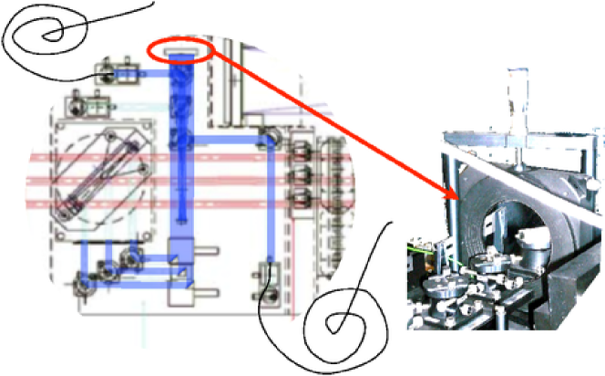
3.2.2 Alignment of the pupil and adjustment of the focalizer
All pupils were properly adjusted in order to match the cold pupil mask and the beam position launched by all the H and K dichroics and the J mirrors. It corresponds to optimized values of the flux while inserting the cold masks (3T_K and 3T_JHK). After the operation, all the translation stages of the mirror or dichroic support were no longer at the limits of their possible strokes. During the same operation we properly aligned the last parabolic mirror (focalizer). The warm optics adjustment improved significantly the image quality. All 0th order images in J, H, and K are smaller than pixels and the image angle is (see appendix B for details).
We recommend that this focalizing mirror must not be used for beam adjustment on the spectrograph slit, but the periscope mirrors instead.
3.2.3 Optical ghosts
Appendix C shows that in the data processing a major problem came from a mismatch of the photometric calibration. We analyzed the historical data acquired prior to the Feb 2008 ATF run as well as new data taken during the run.
We found that there is a residual ghost at a 6% level in the interferometric channel. The remaining ghost is most probably due to internal reflexion inside the spectrograph dewar and it cannot be removed by any alignment of the warm optics. The effect of the ghost can be fully corrected by the software described in Sect. 2 and Appendix A.
We recommend to implement the compensation of the interferometric ghost effects in the amdlib library and to identify some quality checks for the P2VM calibration.
3.3 Optical stability
The stability of the instrument has been an issue for a long time. Therefore we tried to characterize this stability during the ATF run.
3.3.1 Stability of output beams
We have taken daily the position of the beams on the detector with no spectral resolution in order to detect possible drifts. During this survey, no significant drifts were observed within a time scale of a few days. During all this period, we did not perform any adjustment of the optics located after the fiber outputs in the laboratory. Day by day survey of the beam positions and beam fluxes are reported in appendix D. Less than 10% contrast losses requires overlaping at the level of 5 pixels in X and of 0.6 pixels in Y. Figure 14 in appendix D shows that during the ATF run the beams were always within specifications. Our understanding is that the effort done by Paranal to achieve a better stability of AMBER by cutting and strengthening the optomechanical elements were fruitful.
I the same appendix D, we have reported an experiment to see if the output beams were subject to vibrations and the definitive answer is negative.
3.3.2 Optical path stability
The OPD is not stable especially after a major adjustment (several tens of microns). Relaxation time is about 1 day also possibly due to the large CAU mirror (see below). In Sect. D.2 of appendix D, we show that 2 P2VMs taken respectively at the beginning of the night and this end displays same basic features except for the phase on one baseline.
3.3.3 CAU stability
It has been observed that the large parabolic mirror of the CAU present significant instabilities. After tuning operations on the AMBER table, fluctuations of the OPD are observed for hours, and stable situation is attained again after one day. These instabilities may reach up to 100 nm on 1-3 baseline. These fluctuations are directly observed under slight knocking of the mirror support (see Fig. 18), and are present each time a noise source happens on the AMBER table (BCD movements, CAU motor movements certainly, large piezo movements…). We suspect that photometric noise (due to changes in injection in the fibers) is associated with each vibration of this mirror.
3.3.4 Recommendations
We recommend to avoid any too frequent realignment of the output optics which appears not necessary at all. For the OPD, normally if the translation stages of the input dichroics are not used, they should reach their relaxation position. However, one could implement the P2VM calibration which allow to not depend on the actual OPD. Finally, in order to improve the calibration process, solutions to fix the large CAU parabolic mirror must be found.
3.4 Spectral dispersion
3.4.1 Grating position
The grating motor seems to behave in pre-summer 2007 conditions. It losses steps, shifting globally the images of the camera by a few pixels (less than 20) . This does not preclude operation since the camera sub-windows can in general be positioned according to this shift.
However the software developed in Summer 2007 years to measure the shift and recenter the images on predefined positions on the camera, results in too many calls to the rotation of the grating.
We recommend to update the OS and templates in order to avoid moving the grating more than once per configuration.
NOTE: a recent PPRS, No. 026605 reports that the MACCON board was defective and the change of the board improved a lot the reproducibility.
3.4.2 Spectral shifts
The spectrograph is well-aligned. The spectral shifts between photometric channels and the interferometric ones is characterized and should not be recomputed each time (see appendix E) for details.).
The spectral shift is primarily due the combination of the position of the slit (large, narrow, etc) and of a small angle between the optical components that fold the 3 photometric beams on the camera (3 glued total-reflexion prisms). At the worst, this combination changes only by a small amount every time the spectrograph is opened.
We recommend to stop using the spectral calibration procedure and use the fixed shifts.
3.4.3 Spectral calibration of the low resolution JHK mode
We performed a Fourier Transform Spectrograph analysis of AMBER Low Resolution JHK spectra by moving incrementally by steps of 0.01 microns the piezos on beams 1 and 3 for each band (see appendix E). Each pixel of the Interferometric region on the camera of AMBER (32 by 60 pixels in this LR mode) is thus modulated with a period equal to the wavelength it sees. The Dispersion law is found compatible with a linear dispersion of coefficients, , with i as the pixel number.
3.5 Internal calibration source
For tests, the RAS (Remote Alignment Source) was replaced by a laboratory source directly connected to the K band fiber of the CAU. In this condition, while the K band dichroic of the RAS is bypassed, the modulation of the flux in all photometric channels is significantly reduced and is not detectable any more in the raw data in MR (see appendix F). LR image in JHK in this condition allows a detection for all bands
The two CAU fibers suffer from incorrect superposition, since the JH fiber seems to be moving and requires some readjustments. This misalignment lead to non-zero phase closure measurement on the CAU, with an unstable value (see below Sect. 4.1).
We recommend to remove the CAU dichroic and to use only one fiber as the one for the CAU bypassing the 2 dichroics of the calibrations sources (RAS and CAU).
4 Performance limitations
Our main goal for the AMBER Task Force run was to find the origin of the performance limitations of AMBER. We have performed various experiences until we found the principal origin of these limitations: the polarizers.
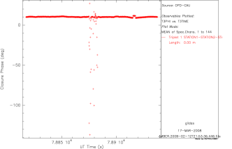
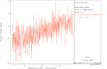
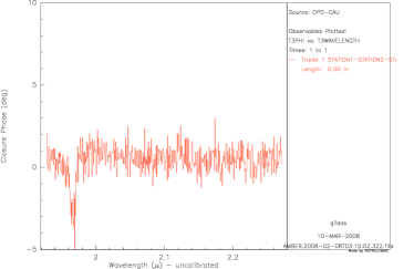
4.1 Closure phase corruption
Previous data set showed that the closure phase signal was corrupted. We realize that by shutting down the remote alignment source (RAS) JH fiber, the K spectrum becomes very different. Residual K band light the RAS JH fiber polluted the K source. Therefore the instrument was seeing a binary made by the strong K fiber and the residual K light going through the JH fiber. By shutting down the RAS light leads to a closure of 0° all over the K band (see Fig. 24 in appendix F).
4.2 Phase beating in differential phase
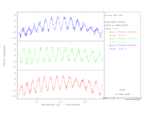
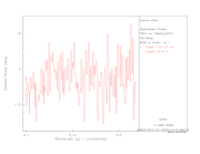
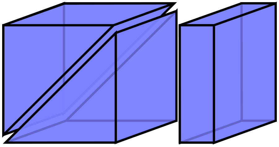
Is called phase beating a periodic oscillation of the phase as illustrated in the left part of Fig. 1. We did intensive tests to find the origin of the phase beating:
-
•
Crossing the fibers. No improvement was found. Crossing does not change injection significantly, but adds a 7.5 mm piston. Although fringes are still visible in HR, there is no significant improvement on phase beating.
- •
-
•
One of the polarizer inserted after the fiber outputs. The polarizer (POL3) placed at the output of the fibers close to the periscope in collimated beams, led to a much higher contrast: 0.9 0.9 0.85 for the different baselines.
-
•
POL3 inserted just before the spectrograph entrance. We put POL3 just before the spectrograph in a convergent beam. It was not successful because although there was a certain gain in contrast, it also generated a lot of unstable flux modulation.
The most probable explanation is a Fabry-Pérot effect (described in appendix H). AMBER documentation provides a description of the polarizers which is recalled in appendix G. The polarizers are made of two prisms separated by an air blade whose thickness is about 120 microns. These air blades can induce a fringe beating in a more complex way than a single Fabry-Pérot effect, because it is not the same in the different arms and leads to additional beating fluctuations both in phase and in amplitude (see for example Fig. 26).
This FP effect cannot be calibrated by the BCD because the fringe shape change too rapidly probably due to the change of the Fabry-Pérot thickness.
We recommend therefore to use other types of polarizers with no parallel optical faces and to use them in a common collimated beams after the fibers.
4.3 Fluctuation of the contrast
The second effect that we investigated is the origin of the fluctuation of the visibilities on sky. These fluctuations seems to be larger than the ones expected because of the atmospheric turbulence. Therefore we tried to identify the hardware on the instrument that could be at the origin of these fluctuations (see log book in appendix L).
We did several experiments:
-
•
Piezos shut down. To check that the piezos were not generating any vibrations, we shut them down. This was not easy, since when plugged off the fiber head are shifted by half stroke (about 40 microns). The input dichroics had to be used to compensate for the differential OPDs. Figs. 30 and 31 illustrate that the visibility fluctuations are still present and even reinforced due to the OPD instability (cf. Sect. 3.5): it could reach 10 to 15%…
-
•
Checking the beam overlap on the detector. One possible explanation could be that due to vibrations the beam overlap is changing with time on the detector. A data set taken with no spectral resolution (see Fig. 16) showed that the beam positions in X and Y but also in flux do not change significantly with time or at a level much less than 1%.
-
•
Data recording with different DIT. Using different Detector Integration Time (DIT), the fluctuations kept the same strength therefore rejecting the possibility to have fluctuations due to vibrations.
-
•
Using the beam commuting device (BCD). No special effect found and also the fluctuations are not reproductive.
- •
-
•
Injection into fibers. The new piezo-controlled ’Iris Fast Guiding’ (hereafter IFG) positioning of the AMBER entrance beams and the availability of the AT beacons were used to test whether the injection of the beam creates or increases the “phase beating” effect. No effects are detectable when the polarizer was removed. In the presence of the polarisers, however, amplitude effects are present and vary in shape with the injection. The small changes in the positioning of the beams demonstrates how sensitive the experiment is to the differential Fabry-Pérot effect induced by the polarizers.
-
•
CAU optical path stability. One possibility for the fluctuations present even without the polarizers is an instability in the CAU subsystem. Monitoring the AMBER observables when touching various mechanical supports of the CAU showed that the large parabolic mirror of the CAU (see Fig. 19 in Appendix D) might be at the origin of some fluctuations. We stopped the investigation in lab and to check what would be the results on sky without using the CAU (see next section).
In conclusion, we believe that the origin of the visibility fluctuations are the results of 2 effects: the Fabry-Perot differential effect changing with time coupled to an instability of a large parabolic mirror in the alignment unit.
4.4 AMBER performance on sky
It is too preliminary to conclude on the overall performances of the instrument, but it seems that even with a reduced instrumental contrast, AMBER limiting magnitude is similar and even better than previously known and can measure small visibilities. The closure phase and differential phases seems to be limited by fundamental (to be checked with SNR calculations) noise and no longer with systematics from the instruments.
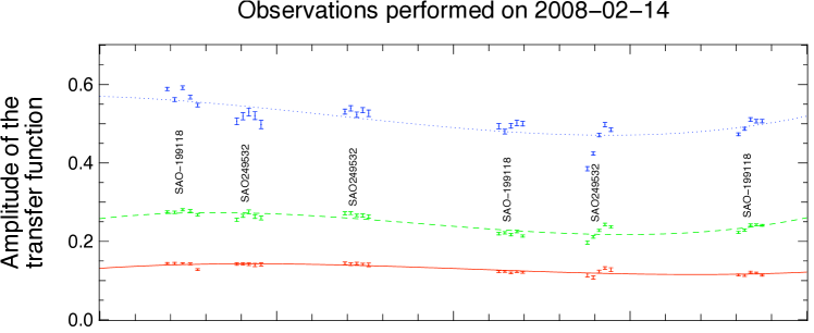
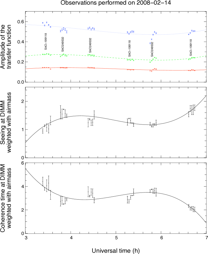
The last night of the ATF run, we have observed repeatedly two calibrator stars in medium resolution without the polarizers together with another star of larger expected diameter. The resulting transfer function is not fully stable, but can be fitted with a polynomial of order 3. The evolution is of the order of less than 5% and can be accounted for seeing (see appendix K).
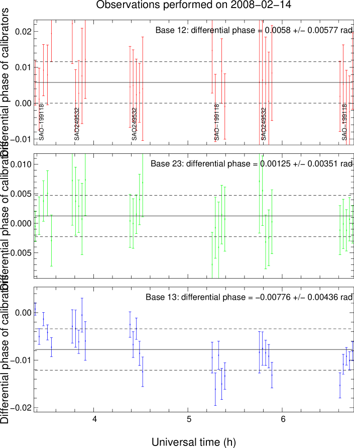
In addition differential phases on all baselines and closure phase are stable all along the night with an accuracy of rad and 5 deg respectively.
Also AMBER has not been tested in all modes, we believe that the polarizers and the CAU mirror were the main sources of visibility fluctuations. We still have low resolution data with and with FINITO to investigate in order to assess the actual performance. However the only assessment which will be valid would be the one made with a new polarizer to get higher contrast.
5 Recommendations
We recommend the AMBER consortium and the ESO responsibles:
-
(1) to take actions as soon as possible to replace the current POL unit with a single polarizer put in the common beam before the spectrograph without Fabry-Perot effect,
-
(2) to investigate the origin of the sensitivity to vibrations of the CAU parabolic mirror and fix it
-
(3) to simplify the calibration light sources (RAS)
-
(4) to fully characterize the instrument in its final state with a final commissioning run
-
(5) to correct the AMBER observing software to minimize spectral grating movements
-
(6) to update the observing software and data reduction pipeline with optimum visibility computation and quality controls.
-
(7) to take the P2VM with a much larger width than the observations ( pixels channel width).
Annexes
Appendix A Data processing analysis
In order to contribute to a better understanding of the AMBER/VLTI system, we have developed an IDL software to model the experimental P2VM, and our own data reduction software, also written in IDL language, to have a full control of each step of the data reduction process which was not possible using the actual amdlib package written in C language.
A.1 Characterization of the AMBER P2VM
The P2VM is fully described by the parameters and by the carrying waves and (see memo AMB-IGR-018 for the definitions [RD 1.3.2], and also Tatulli et al. 2007, A&A 464, 29). The parameters allow to compute the continuum in the interferometric channel from the measurements of the photometric channels. However, the presence of optical ghost (see Sect. 3.2.3) affects the calculation, and the computed continuum does not strictly match anymore the true interferometric channel continuum. To solve this problem to the first order, we introduce a new way to compute the parameters, which takes into account the flux in the 3 photometric channels.
The experimental P2VM is then fitted by a synthetic P2VM. The latter being perfect by construction, the output of the P2VM modelling represents the signature of the AMBER system from the calibration lamp to the scientific detector. This signature can be expressed in terms of 4 observables for each spectral channel:
-
•
the system visibility
-
•
the spatial frequency
-
•
the phases of the carrying waves and
-
•
a continuum regularization parameter
The continuum regularization parameter is introduced to take into account an eventual residual continuum mismatch. If the parameters are correctly computed, then this parameter should be close to 1, which is generally the case with the new procedure.


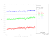
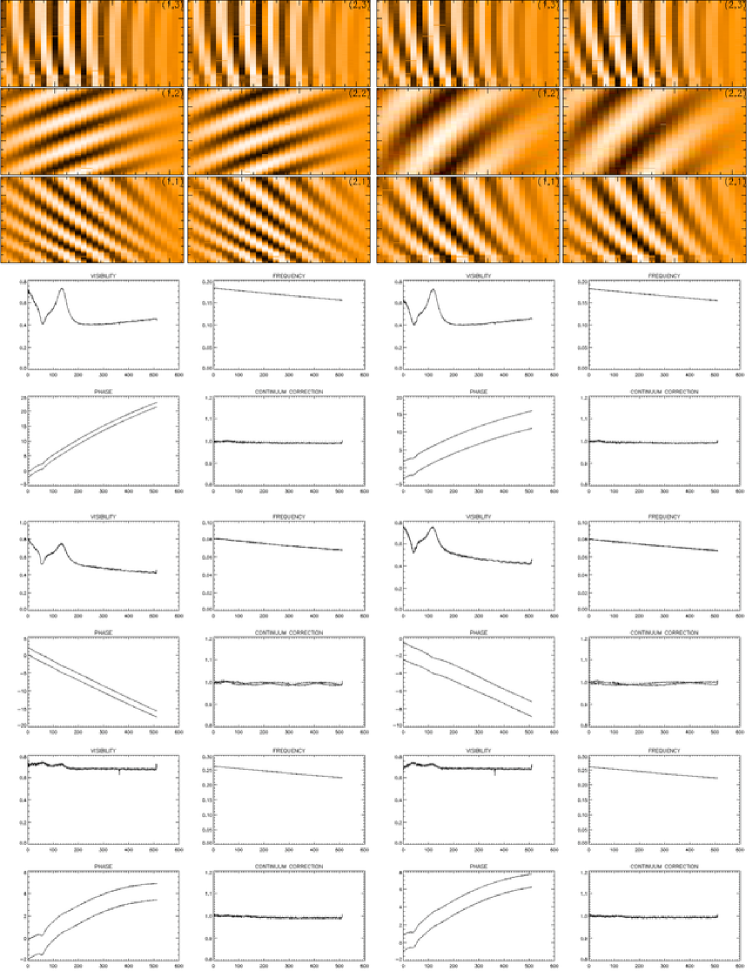
We present the results of the P2VM modelling for 2 sets of data. The first set of data is the P2VM of the Alpha Ara data test set obtained in Feb 2005 during SDT at medium resolution in the K band. The results are plotted in Fig. 3, for each baseline, as a function of the wavelength. At the top we see the system visibilities, with a mean value of about 0.8 beyond 2. Below, we find the spatial frequencies (expressed in pixel-1) whose careful examination (at higher magnification) shows that the spectral dispersion is not constant, but is a linear function of the wavelength. Then, we see the phases of the two carrying waves whose curvatures indicate that interferometric pattern is also curved along the spectral axis. At the bottom, the phase differences between the and are reasonably well within the specifications.
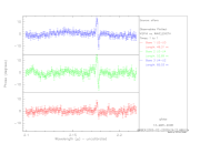
The second set of data is a P2VM acquired on December 29th, 2007, in low resolution mode. The results are plotted in Fig. 4. The low resolution P2VM visibility is in the range 0.5 to 0.8, with large variations from one spectral band to the other. The decrease around 1.5 and 2 is simply due to the superposition of two fringe systems at different spatial frequencies. Also, we may observe some structures within each band. Below, we find the 3 frequency systems and the phases of the two carrying waves. The phase discontinuities between the bands correspond to the observed shifts between the 3 fringe systems. The phase differences are plotted at the botom.
A.2 An improved data reduction software
The characteristics of the new data reduction software are as follows:
-
•
the P2VM is computed as described in the previous section
-
•
a regularization continuum parameter is applied to each interferogram. This parameter is estimated fitting the mean interferogram with 7 parameters (3 complex coherent fluxes and 1 continnum parameter)
-
•
A special attention has been given to the calculation of the covariance matrix of the measurements. The noise resulting from the detector readout noise and the background is estimated from the dark data. The covariance matrix takes into account the correlation between the measurements, and as a consequence is not diagonal. This matrix is inverted spectral line by spectral line.
This new data reduction software has been used to reduce all the data of the ATF run. The detail of the algorithm will be published elsewhere.
Figure 5 shows the relative improvement in S/N for an observation in the test dataset available with amdlib v2.1. It consists of high S/N data taken in good observing conditions in 2005, with the UTs.
The results need a few comments. This is one case where the new algorithm should not produce markedly different results, since the S/N in each frame is strong and statistics are dominated by the vibrations of UT+VLT presents at this date. We forced the spectral displacement values obtained in sect. 3.4.2 for both data reductions, since this is the good value to use, whereas the standard (pipeline) reduction would have used quite different values. The prescribed standard data reduction, in particular in this UT case where vibrations were present, calls for frame selection, however results with the new software are obtained without frame selection (hence the lower visibilities). The gain in S/N is partially due to this, and is more striking in the phase closure.
A.3 On the P2VM spatial extension
The P2VM, as its name suggests, is the mean to convert pixels intensities to correlated fluxes. Its spatial extension on the camera needs not, and should not, be restricted to the 32 pixels wide strips used for the observation.
We have checked that restricting the P2VM extension to the 32 pixels is not harmful in terms of loss of information, since the 6 independent parameters of the 3 simultaneous complex correlated fluxes are more than sufficently fitted on 32 independent pixel values (24 would suffice in theory).
However, we found that in the current AMBER setup where the characterization of s and s depends on the phase induced by an air blade of variable properties (temperature, humidity, repeatability of piezo), one needs the best possible determination of this phase. Errors on this phase measurement will convert into power wrongly transferred between the real and imaginary parts of the instantaneous complex coherent flux proportionally to the piston and the piston jitter.
To minimize the errors in this phase measurement, one needs to measure by an integral method the phase between the s and s with the maximum possible spatial extension, at least 64 pixels instead of the current 32 (TBC).
Appendix B Optical alignment
B.1 Adjustment of the DET/SPG focus
While the dewar was open for maintenances on DET and SPG, we had to adjust properly the focus and tilt of the camera with respect to the spectrograph. A first alignment done during the cooling of the spectrograph was not sufficient.
This alignment is done using the Cold Stop slit at the entrance of the spectrograph, imaged on the camera in normal cold conditions (see Fig. 6). Before starting the alignment, the two brakes of the tuning device must be released (4 screws each beneath the support). The brakes are located on the bottom of the cryostat support on each side. It is better to completely release also the two guiding spheres (3 set of large guiding screws) that allows the three rotation around a point close to the detector. The upper sphere guides the rotations around the optical axis (horizontal axis driven by the 2 vertical screws) and the tilt of the detector (around the vertical axis using the 2 horizontal screws). The lower sphere allows the tip around the horizontal axis within the plane of the detector.
The focus is performed using the long screw located beneath the support (using a key #7 (tbc)) . The focusing is monitored while the slit is imaged in the middle of the detector (0 order / cold stop / Pupil Technics) with a flat illumination (a flash light). The orientation of the slit on the detector is adjusted to be parallel to the columns of the detector.
The tip-tilt is monitored while moving the slit image from one side of the focal plane array to the other one using the movement of the grating. The slit image must be lower than 2 pixels at the center, and must be enlarged by the same amount on the two sides.
In the present case, the previous alignment, due to the lack of time after the maintenance of the grating turret, was probably done before the whole assembly was properly cooled down.
We adjusted the setting to achieved the required tuning, and achieve a 2 pixels large focusing of the cold stop.
Note: doing this measurement one can observe a duplication of the interferometric beam slit, corresponding to a parasitic image (see Fig. 6). Latter measurements showed that this ghost induce fringes in the beam 2. The translation of the ghost with respect to the interferometric beam is 2 pixels down and around 2 pixels to the left side.
B.2 Pupil alignment and focaliser adjustment
The focaliser mirror was completely re-aligned, considering the wrong position of all of its tuning knobs and its obvious misalignment. The alignment start by putting all setting in medium position, which consist in removing all apparent angle of the parabolic mirror with respect to the optical beam. The tilt of the beam image on the camera (spectro set at zero order) can be due to the tilt of this parabolic mirror. It must be noticed that this mirror must NOT be used to adjust the position of overall beams on the SPG entrance slit. This setting must be done using the 2 translation stages of the periscope, one on each mirror that correspond to the 2 directions.
During this alignment we corrected pupil vigneting on the previous 45° mirror where beam 2 and 3 were obscured by its mechanical mount. To correct this vigneting it was necessary to adjust the dichroic angles (output K dichroic in this case). The correction was performed using the dichroic tip-tilt of the beam K2, and then all dichroics where adjusted with respect to the new position of the output K2 dichroic. It was performed an adjustment of the beam print on the 3TK cold pupil inside the cryostat in order to reach the higher signal. In the mean time we determine the correct position of the 3TK pupil mask (-44804 position). It was determine by a maximization of the flux in the image. At the end of the procedure:
-
•
Image position is tuned using the angular tuning of the dichroic, and maximizing the image flux
-
•
Pupil position is tuned using the dichroic translation and maximizing also the image flux
-
•
Check of the image position (and adjustment with angular adjustment)
-
•
Check of the pupil position using the Pupil imaging lens of the detector (manual knob on the detector). The pupil image through the mask is not overlapping the pupil print as seen with a wide field illumination of the spectrograph (flash light)
Doing the alignment of the focaliser we improved a lot the image quality of all the beams. For all J H and K beams the images on the camera are lower than 25x2 pixel with a mean spot angle of 179° (between 178 and 180).
All H and K pupils were then adjusted to fit the 3TK and 3TJHK pupil mask using the adjustments of the H dichroic beam splitters for H band, and the adjustments of the J mirrors for J band (tilts for image positions and translations for pupil adjustments while checking the flux level). In all cases the flux reduction while introducing the pupil mask do never exceed 5% with respect to the images without any pupil mask (see tabled values).
The optimized value for the two masks are now entered in the ICS.
-
•
3TK mask position: -44804,
-
•
3T JHK mask position: -27330
Doing the pupil adjustments, most of the translation stages acting on the OPD were released toward their medium position and no translation stages are not any more in extremal position.
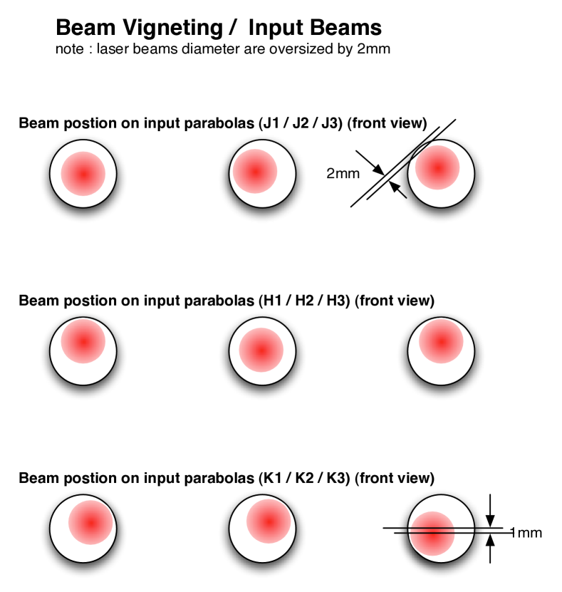
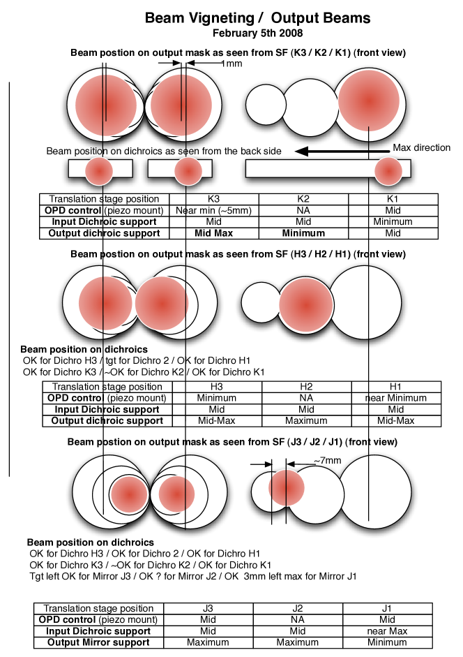
The figures report the positions of the beams on the the input parabola (see Fig. 7) and on the pupil alignment mask located at the output of the Spatial Filters (see Fig. 8).
It must be mentioned that this alignment requires to proceed accurately taking into account all related parameters, using the input and output dichroic translations and the piezo actuator support.
-
•
Piezo support is an independent support, but its translation may strongly affect the beam injection, due to its poor guiding capability. Be aware that if the flux is lost in the fiber, the process is heavy to ge it back.
-
•
Input dichroic translation affect the beam position on input parabolas
-
•
output dichroic translation affects the pupil position on pupil mask in the cryostat. It may also introduce vigneting for related beams (the beam itself, the adjacent ones, and the transmitted beams (for instance H and J on the K dichroics).
For SFJ, it was noticed that the J1 mirror does not allow to put the beam in the theoretical position of the design. If one need to put it in a correct position in order to achieve the correct arrangement of the J pupil, the mirror mount must be translated horizontally along the mirror surface plane. This adjustment requires to drill a new hole for the fixation of this mirror.
Appendix C Characterization of ghosts
C.1 Mismatch of photometric calibration
The acquisition of the P2VM (pixel-to-visibility matrix) is pivotal in the observing and data reduction scheme of AMBER. Immediately after P2VM calibration, every possible calibration parameters have been obtained. The quality of the raw data observations needed to acquire a P2VM do not obey the prerequisites implied by the concept of a P2VM, described by its mathematical formulas.
In brief, the photometric calibration allows to substract the continuum from the detected fringes so that the continuum-corrected interferogram is on average equal to zero. The first problem was found when we compared in the continuum obtained actually measured in the interferometric channel from the one which is being substracted. Fig. 9 shows an intereforgram which has been averaged over 1000 frames. Since the fringe phase fluctuations are larger than a fringe period, the fringe modulation disappears and we got a good estimation of the fringe continuum (black line). On another hand, using the P2VM calibration files which allow the ratio between each photometric beam and its counterpart in the interferometric channel to be measured, one see that the computed continuum (red line) does not correspond to the actual continuum.
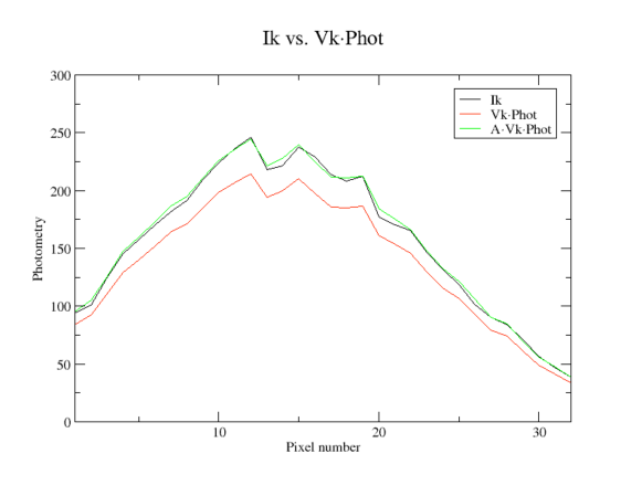
The reason for this mismatch is that the assumption that there is no leaks or ghost in other channels is no correct. One way to compensate this is to introduce a multiplicative factor , or even better to take into account the cross-talk between the channels in the interferometric/photometric ratios (see Sect. 2 and appendix A).
C.2 Investigating P2VM calibration files prior to Feb 2008
 |
 |
 |
 |
 |
 |
 |
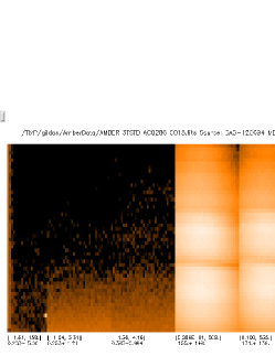 |
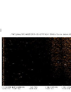
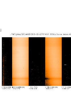
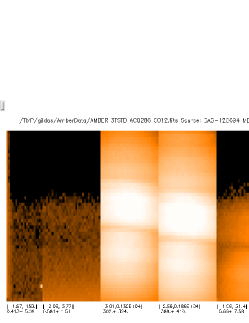
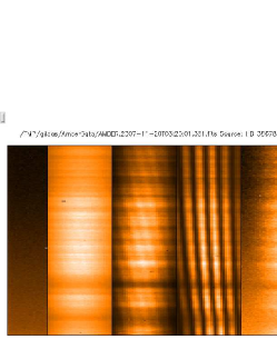
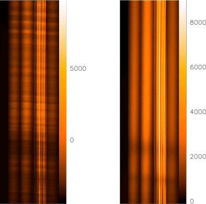
We have analyzed historic data set to investigate if it possible to detect this cross-talk or ghost in the calibration files produced by the P2VM procedure. Figures 10 and 11 shows two data sets taken respectively in Feb 2005 and Sep 2007 just after the SPG intervention.
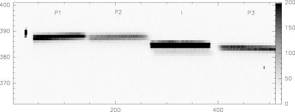
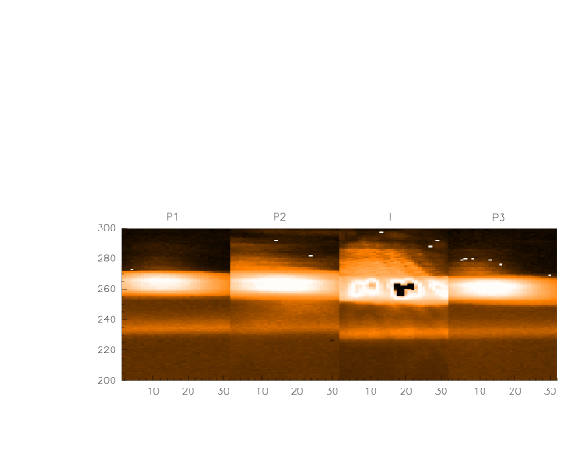
In the following, all images were taken on a mean of all frames in the files. All plots are done with a logarithmic transfer curve to flatten the dynamics. Black is 0.1 ADU, white is 1000 ADU. On all presented images, from left to right we have :
-
1.
masked channel (20 pixels wide, never illuminated)
-
2.
Photometric Channel 1 (32 pixels wide)
-
3.
Photometric Channel 2 (idem)
-
4.
Interferometric Channel (idem)
-
5.
Photometric Channel 3 (idem)
The vertical axis shows the spectral signal from shorter wavelength (bottom) to longer wavelengths (top) for LR mode, the reverse for MR mode. Due to a bug in the gildas interface to the amdlib software used here for displays, the wavelength information on the right of the boxes is incorrect for LR mode.
In Feb 2005 data (Fig. 10), one detect a pollution of beams 1 and 2 by beam 3 at the level of 1%. The example given is done with the “Old” Camera, in mode 3T Medium K. Relevant comments are made in the label of each figure. We note that since this dataset was used for the P2VM of the successfull Alfa Arae data, the effects depicted here were not seen at the time and thus acceptable.
In Sep 2007 data (Fig. 10), beam 2 pollutes beam 3 clearly at the level of 2%. Theses calibrations were done with the “new” Hawaii camera (no remanence) in mode 3T Low_JHK. Note also the position of the dark limit between H and K, and its displacement in beams 1 and 3 wrt the position in beam 2 (enormous with today’s tilted slit). This displacement is not the same in all beams, so the crosstalk between beams is also a crosstalk between wavelengths. It will be difficult to get accurate visibilities with such a crosstalk.
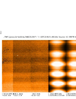
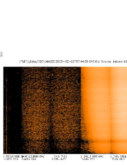
A different type of problem is seen in a second set of observations taken in Medium_K mode (see Fig. 12). In the dark exposure taken before the three files used for computing the spectral displacement (left panel), we note fringes in the interferometric channel. These are due to a remnant feature of the previous observation. It would seem that the camera still has some remanence. Since this kind of frames is used to compensate for pixel biases, any degree of pollution by artifacts will have a severe effect on all the observations. It is advisable to introduce in the AMBER OS a test on each such frames invalidating the data in this case.
In the middle panel of Fig. 12, which shows the beam #3 enlighted with a spectral modulation for teh spectral calibration, the flux variations in the lighted channels (I and P3) change the background in all the other channels, even the masked channel. This is not due to beam pollution but is a know effect of the camera readout, seemingly unavoidable and possibly not entirely taken in account properly in the cosmetics performed in the first steps of the data reduction.
In the right panel of Fig. 12, fringes are visible in the photometric beam 2, and possibly beam 1. Light in beam 3 is due to pollution by beam 2 as in middle panel. The fringe pattern shifts with the piston, proving that this effect is either a global interference pattern in front the camera, or a ghost of interferometric beam seen in beam 2.
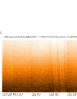
C.3 Ghosts measured during ATF
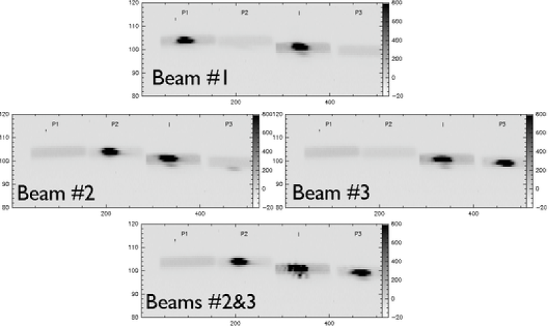
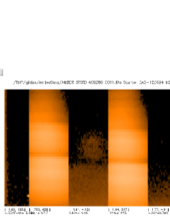
All images have been taken with the narrow slit, in the order of the grating and a neutral density 10 on the CAU lamp to enable a longer integration time. This long integration time enables the visualisation of the slits itself, even in beams where the shutter is closed, thanks to the background thermal emission of the lab going through the slit.
The images of Fig. 13 show that the slit is very well imaged on the camera, and that the dispersion position enable to measure very accurately the beam displacement between the photometric and interferometric beam.
Beam #2 has a clear ghost (6% of flux) in beam #3 (displacement: 2 pixels below). Beam #1 may have a hint of a ghost in #2.
All beams induce a ’second image’ in the interferometric beam (2 pixels below). This double image being common to all beams must arise in internal reflections in the beamsplitter. When 2 beams are lit, as in the #2-#3 image we have a second set of (less bright) clear fringes 2 pixels below the first one. This ghost represents 6% of the incoming flux (but its relative importance may change with the wavelength when the flux is dispersed, as it is in normal AMBER operation). The differential path of these reflections in the beamsplitter being small, the fringes are just displaced by lambda/4.
When we add dispersion, the interferometric channel will thus see superimposed 2 sets of fringes, the normal one plus a second, much fainter, with a different phase, one spectral resoultion element (2 pixels) below. Normally this displacement should not change with the spectral dispersion.
We have been able to take into account quite sucessfully the presence of the ghosts in the data reduction tools we developed specifically for this ATF run (see Section 2), and these algorithms should be ported to the standard data reduction tools for optimal use of AMBER. However this software compensation cannot reach the same level of precision that would be attained by replacing the optical element which creates the ghost if the first place333which remains to be identified.. In particular the ghost fringes seen above cannot be compensated by software and will induce at minimum a contrast loss.
C.4 Conclusions and recommendations
The most probable explanation of the observed ghosts is the effect of the device inside the spectrograph dewar that arranges the beams on the camera. A set of three small adjacent mirrors redirects the 3 photometric beams on the detectors. The widths of these mirrors is very close to the width of the incoming beams and a small misalignment of one of the pupils on these mirrors lead to a leak to the adjacent mirror. According to the pupil alignment, a different amount of leak may occur, and it seems that the last pupil alignment in October 2006 introduced a larger leak on the beam 3. In any case it is not sure that the beam is not a little bit larger that the element-mirrors leading to a slight ghost on both adjacent mirrors.
This ghost effect should be measured and compensated by the amdlib software for the P2VM calculation. However, the large displacements in data taken between Sep 07 and Jan08 are not retrievable easily, at least not automatically (perhaps can be entered by hand), and will reduce the number of useable data channels. Removal of these ghosts and removal of the spectral displacement is badly needed. Besides, we need to have a value returned by the amdlibComputeP2VM routine used in the amber observation software to tag invalid P2VM observations which exhibits ghosts effects above a sensible value (0.5% for example).
The new alignement performed after the Jan 2008 SPG intervention allowed to decrease the cross-talk between photometric beams, but a ghost remains in the interferometric channel which comes from the interferometric channel itself (probably a reflection on the common beamspliter used to extract photometric beams).
The camera change is believed to have solved the remanence problem, although we seem to see the contrary in fig. 12 (upper panel). At the moment, no remanence is taken into account in the data reduction program, for lack of removal method (before or after which cosmetics, with what value, etc…).
Appendix D Optical stability
D.1 Output beams
D.1.1 Medium term stability survey during the ATF operation
A survey of the beam positions and of the beam fluxes was performed during the last week of the ATF operation. No significant drifts were observed within a time scale of a few days. In any case during the second part of the ATF operation, when the main alignments were completed, we did not need any more intervention in the laboratory to re-adjust the beams. Mainly it must be noticed that for the output beams the requirement used by the Paranal team for the adjustment is overestimated. Using the related software alignment tool, the green dot means that the beam is properly aligned, the orange one means acceptable, a re-alignment can be required latter, and only the red dot imposes an immediate re-alignment. It is highly preferable to perform the verification from a control room and to avoid any disturbances on the bench.
Left and middle panels of Fig. 14 show respectively the variation of the beam positions in K, H and J in the X and Y direction, and the right panels display the variation of output fluxes for the diffrent bands. This survey was performed from February 6th to February 13th. On February 12th, the polarizers were removed explaining the significant improvement of the flux level.
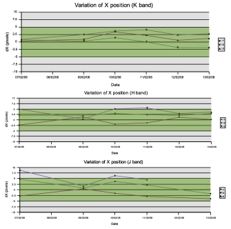
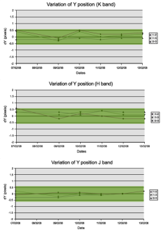
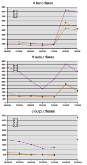
On Fig. 15, we plotted on the left the beam shapes for a typical value of FWHM of 23 pixels in X-direction (solid line) and of 1.6 pixels in Y-direction (dashed line). On the right part of the figure is represented the contrast loss due to overlapping mismatch in pixels. One see that less than 10% losses requires overlaping at the level of 5 pixels in X and of 0.6 pixels in Y. The fact that the positions are within the green zones in Fig. 14 shows that during the ATF run the beams were always within specifications.

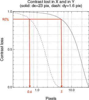
Our understanding is that the effort done by Paranal to achieve a better stability of AMBER by cutting and strengthening the optomechanical elements were fruitful.
D.1.2 Sensitivity to vibrations
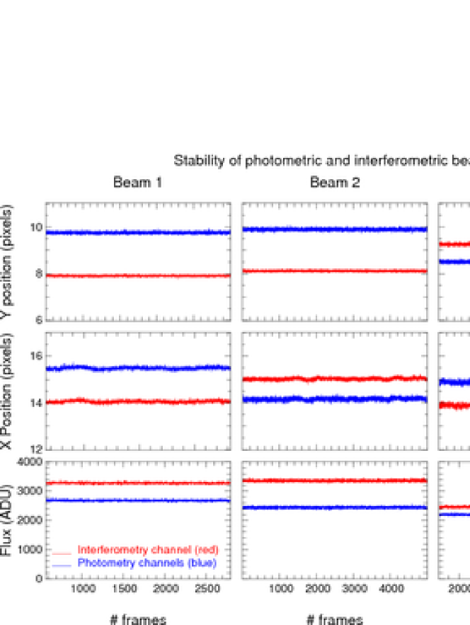
When we were looking for the origin of the fluctuations of the visibility (see Sect. 3.3.1), we have recorded a set of 1000 frames with the grating in the 0th order in order to monitor at relatively high frequencies (more than 10Hz) the motion of the output beams.
The result of this test is reported in Fig. 16. The variations are at maximum within a fraction of pixels, unable to explain visibility variations of a few percent. We concluded that the output beams are not responsible of the visibility variations seen.
D.2 P2VM stability
The stability of calibrations beams have characterized during the last ATF night (see Fig. 17). Left subfigures correspond to the P2VM acquired at the begining of the night, whereas the right ones to the end of the same night. The images at the top of the figures shows the carrying waves. Fringes of baselines 1-2 and 1-3 have not moved significantly whereas the fringe of baseline 2-3 show different pistons. However the analysis of the P2VM using P2VM modeling reported in graphs below show that the envelope and frequencies have not changed. Only the phase has changed.
This is due probably to translation stages of the input dichroics which have been found very unstable. This is a well known problem reported in some PPRS. When used too many times, then the OPD is unstable. However we think it would be possible to make the P2VM calibration process unsensitive to the piston so that this problem should not be a problem. This needs further investigation.
D.3 CAU stability
We did a series of experiment on the CAU to test its stability. During the search for the origin of visibility fluctuations, we noticed that the visibility measurements were very sensitive to some elements of the CAU, especially the large CAU parabolic mirror.
In Fig. 18, we have recorded an exposure (1000 frames) on the CAU source while touching different mechanical supports of the CAU. We found that the mount of the large CAU parabolic mirror (identified on Fig. 19) was very sensitive to mechanical impacts. We think that it may be the source of the instabilities seen when we were looking to the effect of polarizers (see appendix G).
D.4 Conclusion: on alignment requirements and health checking
We recommend to relax the alignment requirements to 8 pixels (see fig. 15), in order to avoid too frequent interventions in the laboratory. However, this requirement holds for each pair of beams, at each wavelength. We recommend that in the p2vm computation a fit of the position of each beam, as seen in the interferometry channel, as a function of lambda, be performed, that these values be used as health check, and that a warning be issued each time a significant percentage () of wavelengths are above these specs.
We also recommend to check the fixation of the large CAU parabolic mirror.
Appendix E Analysis of the spectral resolution
E.1 Spectral shifts between photometric and interferometric channels
The spectrograph is well-aligned. The spectral shift between photometric channels and the interferometric ones is characterized and should not be recomputed each time (gain of observing time).
The spectral shift is primarily due the combination of the position of the slit (large, narrow, etc) and of a small angle between the optical components that fold the 3 photometric beams on the camera (3 glued total-reflexion prisms). The figure 13 show such images of the slit. At the worst, this combination changes by a small amount every time the spectrograph is opened. To our knowledge, this defines only 3 periods: 2004–Sep, 2007; Sep, 2007-Jan, 2008 and Feb, 2008–present.
The repositioning of the slit by the slit wheel motor seems (TBC) to be sufficiently accurate to insure that the slit+folding device setup did not change during these periods.
The displacement of the image of the slit on the camera measures the main displacement. This can be done only once each time the spectrograph is opened, and could be done in the following manner:
-
1.
take 3 exposures full frame images of the narrow slit, one beam lit at a time, grating at 0 order.
-
2.
sum each image on the X axis (taking care of bad pixels. Flat is not needed)
-
3.
on these 3 vectors, fit two gaussians of FWHM. Their position will serve as a marker of the position of each beam;
-
4.
average a few long (1 min) exposures full frame images of the narrow slit, all shutters closed;
-
5.
extract 4 strips in the Y (lambda) direction, of 64 pixels wide, centered on the positions of the beams found before (taking care of bad pixels. Flat is not needed);
-
6.
sum each strip on the Y axis, fit a gaussian (of a few pixels wide) in each. The displacement of the gaussian positions of strips 1,2 and 4 wrt. strip 3 is the displacement sought. The width of the gaussian is an indication of the quality of imaging of the slit onto the camera (hence the spectral resolution).
-
7.
to evaluate the quality of the focussing of each beam the same procedure can be reproduced with one beam lit at a time.
We have done measurements during our ATF stay, and have found old images of the slit taken in 2004, permitting also this kind of measurement. Table 1 summarizes these values.
| Period | P1 | P2 | P3 | Notes |
| 2004-Aug2007 | +0.873 | +2.064 | +0.472 | 1 |
| Sep2007-Jan2008 | +2.000 | +2.576 | +0.263 | 2 |
| Feb2008-Present | +3.008 | +2.850 | -1.319 | 3 |
| Notes of the table: 1. These 2004 values seem to hold at least until 2005 Feb. It is necessary and easy to check that it holds until Sep07. 2. Based on Nov07 measurements (SPECPOS frames). Slit was very tilted and slit badly focussed (See fig 20 and appendix C comments). 3. Values should be measured again on background-illuminated image of the slit. We believe these are however good values for data reduction purposes. | ||||
The 2004 values seem to hold at least until 2005 Feb, 25 since they work well with Arae measurements (see Fig. 21). It is necessary and easy to check that is holds until Sep 2007.
During the replacement of the infrared Hawaii detector in Sep, 2007, a slight defocus and tilt of the slit image was introduced, which was not corrected until Feb, 2008. During this period, the image of the slit on the camera worsened severely, as seen in fig 20. Such defocussing of the slit induces a loss of spectral resolution, and the extenuation of the visibility with the piston (sect. E.3 worsens: in LR mode, the maximum tolerable piston drops to microns.
Please note, that subpixel shifting, as it is done in amdlib (and the author does not see how it could be done otherwise) introduces biases in spectrum and P2VM in presence of bad pixels. We recommend to use integer pixel shift for the moment. (, , for the old data,, , for the sep07-Jan08 data ).
In operation, three anamorphed beams pass through the slit. These beams are, if amber is correctly aligned, highly elongated ellipsoidal flux distributions tilted with a very small angle () wrt the slit, whose shape can be measured at 0th order with a good precision. Thus, one could in principle apply psf deconvolution on the P1, P2 and P3 spectra, possibly to gain in spectral resolution in the spectrum. It remains to be proved that the same could be done in the I channel, taken into account in the P2VM fitting process, and provide a sensible improvement in the results.
E.2 Spectral calibration in low resolution JHK mode
We performed a Fourier Transform Spectrograph analysis of AMBER’s Low JHK spectra by moving incrementally by steps of 0.01 microns the piezos on beams 1 and 3 for each band. Each pixel of the Interferometric region on the camera of amber (32 by 60 pixels in this LR mode) is thus modulated with a period equal to the wavelength it sees. Furthermore the visibility of the 1-2 and 2-3 fringes will vary as a function of piston and will change as the fourier transform of each spectral channel shape.
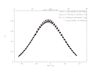
We acquired four observations of images, covering piezo displacements of with resolution, with the polarizer present, so the data is perturbated by the phase beating effect depicted in Sect 4.2, and the dispersion law was thus obtained for the H and K regions of the spectrum only. A typical result is depicted in fig. 22, where the phase beating perturbation is clearly visible.
The Dispersion law is found compatible with a linear dispersion of coefficients:
with i as the pixel number.
E.3 Calibration of visibility losses due to temporal coherence
Table 2 presents the ’equivalent coherence length’ of the extenuation of as a function of piston ’opd’. It has been computed through the K band by fitting the extenuation law in sinc expected from a square spectral channel of bandwith and
Table 3 is a subproduct of the data reduction used in the measurement. It shows the maximum piston measurable with the Low_JHK spectral resolution in case of good S/N.
| LR Spectral | ||
|---|---|---|
| Channel number | (microns) | (microns) |
| 1 | 2.6596 | 46 |
| 2 | 2.6275 | 51 |
| 3 | 2.5954 | 53 |
| 4 | 2.5633 | 52 |
| 5 | 2.5312 | 51 |
| 6 | 2.4992 | 52 |
| 7 | 2.4671 | 55 |
| 8 | 2.4350 | 58 |
| 9 | 2.4029 | 59 |
| 10 | 2.3708 | 58 |
| 11 | 2.3387 | 57 |
| 12 | 2.3066 | 55 |
| 13 | 2.2745 | 57 |
| 14 | 2.2425 | 59 |
| 15 | 2.2104 | 59 |
| 16 | 2.1783 | 56 |
| 17 | 2.1462 | 58 |
| 18 | 2.1141 | 57 |
| 19 | 2.0820 | 59 |
| 20 | 2.0499 | 50 |
| 21 | 2.0179 | 54 |
| 22 | 1.9858 | 58 |
| 23 | 1.9537 | 33 |
| Band | Maximum Measurable Piston |
|---|---|
| Channel number | (microns) |
| J | |
| H | |
| K |
Appendix F Internal light sources and effect on closure phases
F.1 Analysis of internal sources
We investigated how the CAU sources, also called RAS, could be simplified and understood. We explain below some tests which were performed.
-
•
RAS dichroics effects: For tests the RAS has been replaced by a laboratory source directly connected to the K band fiber of the CAU. In this condition, while the K band dichroic of the RAS is shunted, the modulation of the flux in all photometric channels is significantly reduced and is not detectable any more in the raw data in MR (see Fig. 23). LR image in JHK in this condition allows a detection for all bands. The signal in J and H bands is then highly affected by the fact that the CAU dichroic acts in this test setup, in reflection while it is supposed to be operated in transmission for this spectral range. One can retrieve the reflection curve of the dichroic presented in VLT-TRE-AMB-15830-1010 section 9 (AMBER OPM test report).
-
•
CAU fibers: It has been observed for a long time by AMBER operators than the 2 CAU fibers suffer from incorrect superposition, as the H fiber seems to be moving and requires some readjustments. This misalignment lead to non-zero phase closure measurement on the CAU, with an unstable value. The measurements done with a laboratory source, shows that a single K band fiber is able to provide the illumination for all wavelengths. Even if the core of the K band fiber can be resolved by the AMBER setup, this effect is properly taken into account by the calibration procedure of the P2VM. If the CAU remaining dichroic is replaced by a mirror, then the flux in all bands are sufficiently balanced with a suitable transmission. We recommend to replace the CAU dichroic and its support by the equivalent mirror and support which deflects the light coming from the H band fiber. Then we keep only one fiber (K band Verre Fluore fiber) for the CAU and to bypass the 2 dichroics of the calibrations sources (RAS and CAU).
F.2 Effect on closure phase calibration
Measurements showed that the closure phase signal was corrupted. We realize that by shutting down the remote alignement source (RAS) JH fiber, the K spectrum becomes very different. Residual K band light the RAS JH fiber polluted the K source. Therefore the instrument was seeing a binary made by the strong K fiber and the residual K light going through the JH fiber. By shutting down the RAS light leads to a closure of 0° all over the K band (see Fig. 24).
Appendix G AMBER polarizers
The polarizers were found to be at the origin of the phase beating and partly at the origin of visibility fluctuations of the AMBER instrument. In this appendix, we describe the polarizers and present some measurements made when looking for visibility fluctuations.
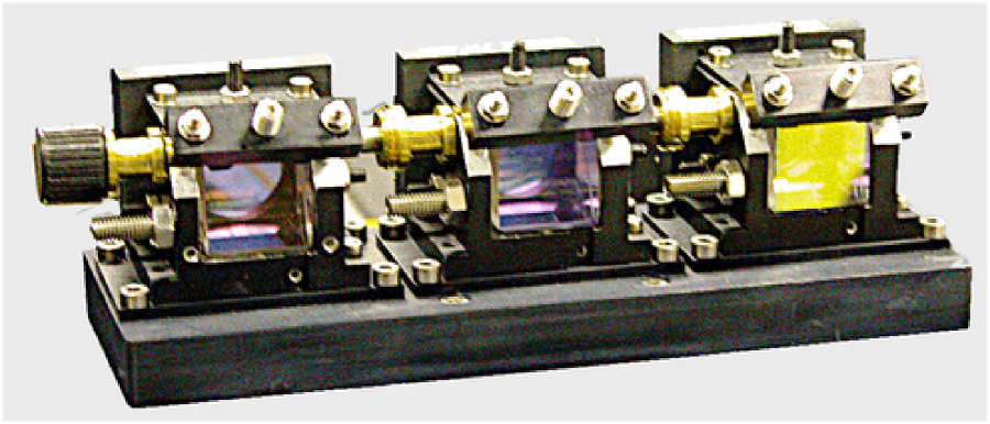
G.1 Polarizers current design
In the OPM Warm Optics Design Report (doc. VLT-TRE-AMB-15830-1001, see [RD 1.3.2]444Available at http://amber.obs.ujf-grenoble.fr/PLAIN/pae/Documents_PAE/Documents/7_TRE_OPMODR.pdf)
3.6 POLarization module
Product tree list : AMB-OPM-POL-(PL1,PL2,PL3)-(POL,CBL)

.../...

The maximum defect with respect to the mean thickness of the 3 blades POL-(PL1,PL2,PL3)- CBL
must be lower than +/-100 microns.

The beam deviation of the delivered polarizer (> 1’) is not compatible with the +/-5"
specification imposed by the differential observations (see OPM LLS [3]). This deviation is
then minimized by the adjustment of the two prisms constituting the polarizer, the two
latter being dissociated. This allows to control the prismatic air layer at the
interface. In addition, to be compatible with the differential chromatic OPD specifications,
a prismatic blade needs to be added for each polarizer.  The complete definition of the
blades is given in the OPM Test Report.

In order to ensure a good parallelism between the two opposite internal faces after the
dissociation of the prisms which constitute each polarizer, a plastic wedge of 0.12 mm is
introduced between these two prisms. The angle formed by this separation needs to be stable
within 3.5" during the observations.
In the OPM Warm Optics Test Report (doc. VLT-TRE-AMB-15830-1010, see [RD 1.3.2]555http://amber.obs.ujf-grenoble.fr/PLAIN/pae/Documents_PAE/Documents/9_TRE_OPMTR.pdf).
13 Manufacturer delivery of the polarizers POL
.../...

13.2.2 After reception of the polarizers

Measurements and simulations were performed by Yves Bresson, OCA. They show that the air
blade located between the two prisms constituents of each polarizer must be parallel in
order for the assembly polarizer and associate compensating blade to respect the chromatic
dynamic OPD specifications. A peeling off of the two prisms constituents of the polarizer
from the initial mounting delivered by the manufacturer was required in order to insert a
plastic shim (with an opening for the optical beam) between them.

.../...
14.3 AMB-OPM-POL optical pre-adjustment
.../...
14.3.2 Principle of the assembly and of the compensation

The polarizer is composed of two prisms in calcite. In order to ensure a good parallelism
between the two opposite internal faces after the dissociation of the prisms which
constitute each polarizer, a plastic shim of 0.12 mm is introduced between these two
prisms. A first prism leans inside the mount on six iso-static points constituted by 3 tips
on the lower plate, 2 others for the orientation and a reference position [4].

The internal face of the second prism leans on the plastic shim via 3 points constituted by
a tip on the lower plate and 2 lateral tips whose one allows the rotation of the prisms
along the optical axis (range : +/- 0.5 mm). This prism is clamped by a corner plate guided
between two sticks with a spring toe.

Considering the characteristics of the prisms in terms of parallelism and thickness
differences, we have inserted compensating blades in order to correct these defaults and to
be compatible with the OPD specifications. These compensating blades are mounted in
cylinders which can be rotated along the optical axis.

Zemax simulations give the associated chromatic dynamic OPD as a function of the optics
characteristics and positions and of the measured beam deviations.
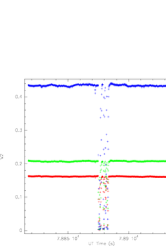
G.2 Influence of polarizers on the AMBER observables
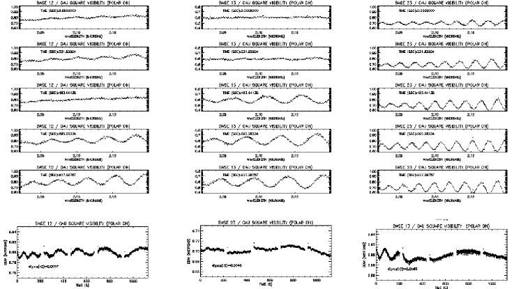
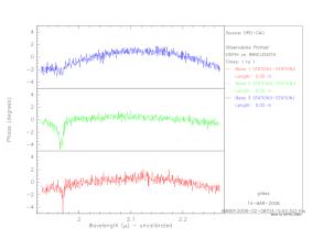
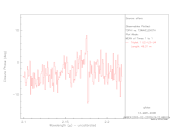
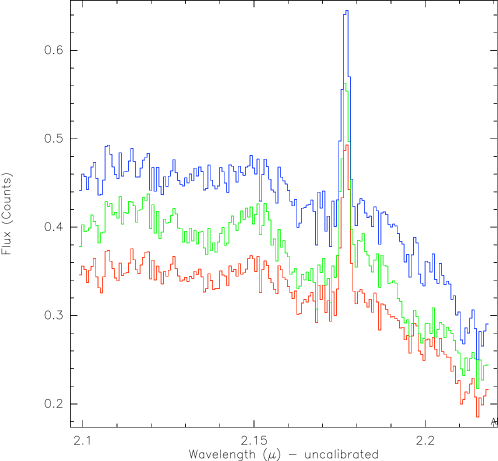
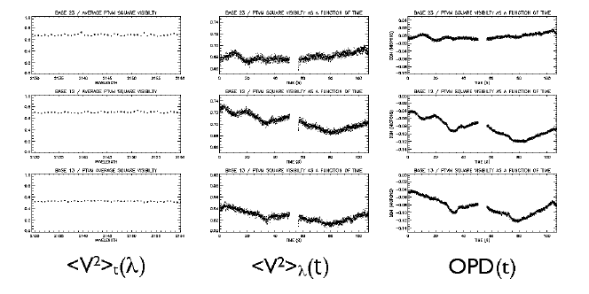
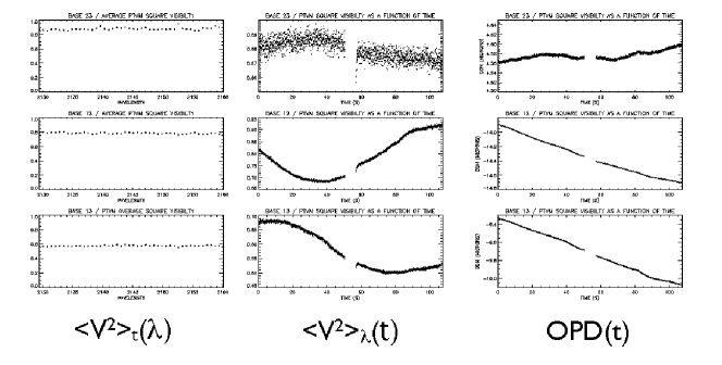
Figures 26 and 27 shows the square visibilities measured respectively with and without the AMBER polarizers. It is interestin to note that the fluctuations of the visibilities seem to come from varying periodic oscillations with wavelength appearing and disappearing in the visibilities. These oscillations disappeared totally when the polarizers are taken out of the instrument. However the averaged visibility decreases to a level of 0.2 or two baselines and 0.4 for the third one.
Our understanding of this phenomenon is that the air blade between the two prisms of each polarizer is acting as a Fabry-Perot interferometer. Applying Eq. (1) to the number of oscillations seen in a Fig. 26 gives the following Fabry-Pérot thickness:
-
•
Baseline 1-2: in gives a thickness of .
-
•
Baseline 1-3: in gives a thickness of .
-
•
Baseline 1-2: in gives a thickness of .
We have performed several measurements and the number of oscillations per spectral bandwidth is changing with time and veries between and , which the order of size of the shim introduced between the two prisms. As a matter of fact, each baseline sees two polarizers and the interferences can create beating effects with a large range of frequency and amplitude.
The fact that the oscillations disappear when the polarizers are taken out is the final proof that these feects comes from the air blade present in the polarizers.
G.3 Where to put the new polarizers?
Polarizers are however necessary to control the polarization. We have dismount POL3 to try to place it in other part of the instrument. When putting it near the periscope in a place where the beam propagation was collimated, we obtained contrast of 0.9, 0.9 and 0.85 instead of 0.4, 0.6, 0.4. Therefore one should modify the instrument to introduce polarizers without air blades. Unless we succeed in understanding why the visibility drops to such low value without polarizers.
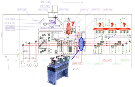
The present location of the polarizers is represented on Fig. 28. The location of the new polarizer should be chosen with great care. On the same figure, we propose two different locations. However, the position of one unique and common polarizer in the periscope tower should be privileged rather than 9 independant polarizers located at the output of the fibers.
Appendix H Fabry-Pérot interferometer principle
[From Wikipedia, the free encyclopedia (http://en.wikipedia.org/wiki/Fabry-Perot)]
In optics, a Fabry-Pérot interferometer is typically made of a transparent plate with two reflecting surfaces, or two parallel highly reflecting mirrors. Its transmission spectrum as a function of wavelength exhibits peaks of large transmission corresponding to resonances of the etalon.
The resonance effect of the Fabry-Pérot interferometer is identical to that used in a dichroic filter. That is, dichroic filters are very thin sequential arrays of Fabry-Pérot interferometers, and are therefore characterised and designed using the same mathematics.
The varying transmission function of the FP is caused by interference between the multiple reflections of light between the two reflecting surfaces. Constructive interference occurs if the transmitted beams are in phase, and this corresponds to a high-transmission peak of the etalon. If the transmitted beams are out-of-phase, destructive interference occurs and this corresponds to a transmission minimum. Whether the multiply-reflected beams are in-phase or not depends on the wavelength () of the light (in vacuum), the angle the light travels through the FP (), the thickness of the etalon () and the refractive index of the material between the reflecting surfaces ().
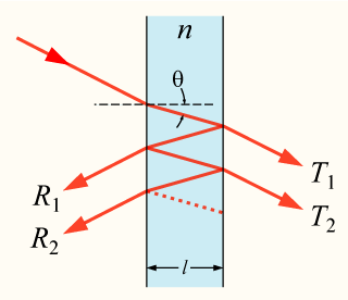
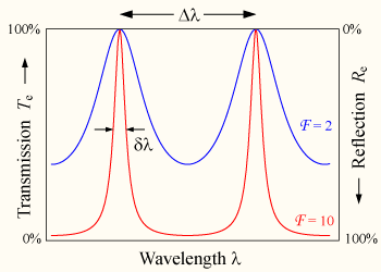
The wavelength separation between adjacent transmission peaks is called the free spectral range of the FP, , and is given by:
| (1) |
where is the central wavelength of the nearest transmission peak.
Therefore the thickness of the étalon is given by:
| (2) |
Appendix I Piezos controling differential OPDs
During the ATF investigation, we were interested to know if the piezos which drives the fiber injection to control the differential OPDs cold be at the origin of vibrations that could lead to visibility fluctuations. We have therefore taken exposures with the piezos on and off (see Figs. 30 and 31). This experoence was made with the polarizers still on the table.
We have not detected any changes in the behavior of the visibility. When the piezos are off then all piezos move by 40 microns at the beginning of the stroke. We had to compensate these OPDs manually with the translation stage of the input dichroics which are known to unstable. Therefore the increase of the OPD changes seen on the right part of Fig. 31 are probably relaxation of these translation stages.
Appendix J Influence of injection into the fibers
We took the opportunity of the new piezo-controlled ’IRIS Fast Guiding’ (IFG) positioning of the AMBER entrance beams and the availability of the AT beacons to test whether the injection of the beam creates or augments the “phase beating” effect (see sect. 4.2).
We found (see Fig. 32) that there is no effect detectable of the changes of injection (up to five core diameters) when the polarizer (Appendix G) is removed. The dispersed spectra of the beacons are devoid of amplitude structures (phase was not mesurable since beacons are not one coherent source), and the flux injected simply diminishes as the injection worsens. In the presence of the polarisers, however, amplitude effects are present and vary in shape with the injection. That the small changes in the positioning of the beams induced by the IFG would produce this effect demonstrates how sensitive the experiment was to the differential Fabry-Pérot effect induced by the polarizer.


Appendix K Observing calibrators without polarizers
The last night of ATF run was focused on the observations of 2 calibrators without FINITO in order to characterize AMBER without the polarizers:
-
•
SAO 199118: diameter of (Bordé), spectral type K2.5 II-III and
-
•
SAO 249932: diameter of (Bordé), spectral type K5 III,
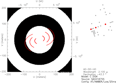
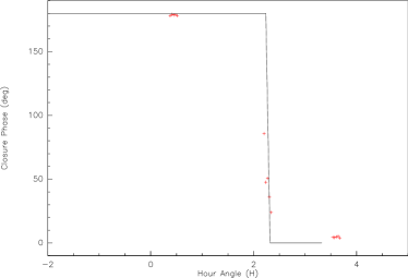
and a larger star SAO 218755. We have reduced these data in order to display the curve of the transfer function (see Fig. 34). We have also computed the differential phase and the closure phase.
The result of this night is:
-
•
transfer function (see Fig. 34): accuracy of the order of the percent. However it changes with seeing conditions and coherence time and therefore calibrations should be done at close as possible from the target science.
-
•
Differential phase (see Fig. 35) are zero at veru good accuracy (less than rad, i.e. within specifications).
- •
During this night, we have interlaced the observation of the star SAO 218755 which has an epxected diameter of 6.4 mas. Interestingly, the longest baseline crosses the first lobe and therefore we were able to see a shift in the closure phase validating the closure phase measurement (see Fig. 33)

| SAO | Time | ||||||||||
|---|---|---|---|---|---|---|---|---|---|---|---|
| Number | (hours) | (degrees) | (degrees) | ||||||||
| 199118 | 0.00 | 0.156 | 0.003 | 0.067 | 0.005 | 0.012 | 0.004 | 0.00 | -0.002 | -0.01 | 55.74 |
| 199118 | 0.04 | 0.141 | 0.004 | 0.065 | 0.005 | 0.011 | 0.005 | 0.01 | -0.004 | -0.02 | 59.51 |
| 199118 | 0.09 | 0.158 | 0.003 | 0.069 | 0.005 | 0.012 | 0.004 | 0.00 | -0.018 | 0.00 | 57.16 |
| 199118 | 0.13 | 0.146 | 0.004 | 0.066 | 0.006 | 0.011 | 0.004 | 0.01 | -0.007 | -0.02 | 56.83 |
| 199118 | 0.17 | 0.135 | 0.004 | 0.060 | 0.007 | 0.008 | 0.006 | 0.02 | -0.002 | -0.07 | 55.90 |
| 249532 | 0.39 | 0.160 | 0.012 | 0.062 | 0.009 | 0.017 | 0.007 | 0.01 | -0.040 | -0.01 | 55.64 |
| 249532 | 0.43 | 0.168 | 0.012 | 0.067 | 0.009 | 0.017 | 0.007 | 0.01 | -0.008 | -0.11 | 58.07 |
| 249532 | 0.46 | 0.176 | 0.012 | 0.072 | 0.009 | 0.016 | 0.006 | 0.02 | -0.007 | 0.04 | 57.67 |
| 249532 | 0.50 | 0.170 | 0.013 | 0.066 | 0.011 | 0.016 | 0.008 | 0.01 | -0.022 | -0.06 | 54.96 |
| 249532 | 0.53 | 0.155 | 0.013 | 0.064 | 0.011 | 0.016 | 0.009 | 0.02 | -0.019 | -0.09 | 56.95 |
| 249532 | 1.01 | 0.180 | 0.009 | 0.070 | 0.007 | 0.017 | 0.008 | 0.01 | 0.010 | 0.10 | 57.18 |
| 249532 | 1.04 | 0.186 | 0.008 | 0.070 | 0.006 | 0.017 | 0.007 | 0.02 | 0.004 | 0.10 | 59.50 |
| 249532 | 1.07 | 0.175 | 0.008 | 0.068 | 0.006 | 0.017 | 0.006 | 0.01 | 0.007 | 0.07 | 58.33 |
| 249532 | 1.11 | 0.183 | 0.008 | 0.068 | 0.006 | 0.016 | 0.006 | 0.03 | -0.009 | 0.04 | 60.60 |
| 199118 | 1.88 | 0.127 | 0.008 | 0.045 | 0.006 | 0.012 | 0.005 | 0.05 | 0.021 | -0.04 | 61.20 |
| 199118 | 1.91 | 0.122 | 0.008 | 0.045 | 0.006 | 0.012 | 0.004 | 0.08 | -0.002 | 0.01 | 60.82 |
| 199118 | 1.94 | 0.157 | 0.008 | 0.082 | 0.006 | 0.038 | 0.004 | 0.05 | -0.140 | -5.08 | 57.71 |
| 199118 | 1.98 | 0.134 | 0.008 | 0.047 | 0.006 | 0.012 | 0.004 | 0.06 | -0.007 | 0.01 | 61.99 |
| 199118 | 2.01 | 0.133 | 0.007 | 0.042 | 0.005 | 0.012 | 0.004 | 0.06 | 0.006 | -0.02 | 62.30 |
| 249532 | 1.14 | 0.178 | 0.011 | 0.066 | 0.009 | 0.016 | 0.010 | 0.04 | 0.027 | 0.09 | 55.29 |
| 249532 | 2.38 | 0.100 | 0.008 | 0.037 | 0.009 | 0.011 | 0.012 | 0.04 | 0.009 | -0.07 | 26.20 |
| 249532 | 2.41 | 0.121 | 0.007 | 0.043 | 0.007 | 0.010 | 0.010 | 0.05 | -0.059 | 0.19 | 46.11 |
| 249532 | 2.44 | 0.149 | 0.006 | 0.050 | 0.006 | 0.013 | 0.008 | 0.04 | -0.004 | 0.09 | 52.37 |
| 249532 | 2.48 | 0.167 | 0.007 | 0.057 | 0.006 | 0.015 | 0.008 | 0.03 | -0.001 | -0.05 | 54.33 |
| 249532 | 2.51 | 0.158 | 0.007 | 0.054 | 0.006 | 0.014 | 0.010 | 0.06 | -0.015 | 0.01 | 51.49 |
| 199118 | 3.23 | 0.146 | 0.005 | 0.047 | 0.005 | 0.011 | 0.005 | 0.05 | 0.010 | -0.06 | 54.59 |
| 199118 | 3.27 | 0.156 | 0.005 | 0.050 | 0.005 | 0.011 | 0.005 | 0.05 | -0.012 | 0.02 | 55.35 |
| 199118 | 3.30 | 0.173 | 0.005 | 0.055 | 0.004 | 0.013 | 0.005 | 0.04 | 0.020 | 0.09 | 57.73 |
| 199118 | 3.33 | 0.170 | 0.005 | 0.055 | 0.004 | 0.012 | 0.005 | 0.04 | -0.007 | -0.02 | 56.69 |
| 199118 | 3.37 | 0.171 | 0.004 | 0.055 | 0.004 | 0.011 | 0.005 | 0.03 | -0.014 | -0.01 | 57.66 |
Appendix L Log book of the ATF run
*  31-Jan to 5-Feb:
    o pupil alignment
    o OPD de-saturation

* 6 Feb:
    o H-band pupil alignment + OPD de-saturation
    o ghost characterization
    o overall stability control

* 7-Feb:
    o find the fringe beating, characterize it at LR, MR and HR
    o Tests: crossing fibers. No improvement. Crossing does not change
      injection significantly, but adds a 7.5mm piston. Fringes still visible i
      HR. No significant improvement on phase beating.
    o remove the polarizers and test at LR, MR and HR: no more fringe beating
      (but lower --by half-- fringe contrast).
          + flux in K much higher and spectrum very different
          + still a phase closure on the CAU of 6
          + We realize that by shutting down the RAS JH fiber, the K spectrum
            becomes very different --> strong K pollution through the JH fiber.
          + Additionnally, now, the RAS light gives a closure of 0 !
    o tests on sky on Sirius in MR and HR with 2 telescopes

* 8-Feb:
    o discussion with RPe on status
    o discussion with Pedro on alignment procedures
    o test of a single fibered source in RAS: strongly reduced flux beating
    o put POL3 after output f fibers close to the periscope in // beams: higher
      contrast: 0.9 0.9 0.85
    o discussion with Andres on software procedures.
    o try some Sirius 3T obs with this setup

* 9-Feb
    o put back the POL3 at its ’nominal’ position
    o AMBER is fully realigned
    o test of an Ocean Optics source in entrance of the fiber K: flux in J and H
      is higher than with normal RAS lamp but there is absorption due to dichroics.
    o tests of piezos: 10mV noise corresponding to 0.1 microns ampltitude
    o Observations on CAU show OPD drifts and visibility fluctuations.
    o laser for spectral calibration: PKe explains to FMa how it works.
    o test on switched-off piezo: it seems that visibilities are higher with
      piezo off than on, but we still see changes of several % in minutes.

* 10-Feb
    o test of the stability of the output beams in 0th-order and also in MR-K:
      conclusion, this is not the reason for the visibility fluctuations.
    o fibers to be inverted: not possible in LR and MR because the OPD
      difference is about 7mm.
    o test with the BCD to identify if the source of fluctuations is before or
      after the BCD: BCD in & out with piezos off in MR.
    o OPD on or off to see differences
    o bang tests in H and K.
    o foreseen: test switching off all motors. Piezos have been shut down.

* 11-Feb
    o different DIT in MR to see the origin of vibrations if any...: no dependance
    o different DIT in H & K LR to see the origin of vibrations if any: no
      dependance -> is there really vibrations?
    o check the CAU source: PKe’s source enlight K, H & J but presence of
      absorption line due to dichroics
    o display the K-LR fringes on RTD and locate sensitive optical parts: the
      large parabola of CAU is very sensitive
    o P2VM? + obs. in LR with no piezo to check that the variation of V^2 come
      or not from piezzos: impossible to do because of OS software
      limitations. P2VM? requires piezo on for l/4 dephasing and the software
      forces them to be at 40um. No piezos means an OPD of 40um.... We stopped.
    o P2VM? + obs. in MR: OK but we have still fluctuations: does it mean that
      piezos are out of questions?
    o Observation with the beacons for bias estimation
    o Scan of the fiber inputs with the beacon to see influence of incidence
      (polarizer on)
    o Polarizer is taken out: no more photometry socks
    o Data reduction of previous data: the fluctuations are large, changing in
      wavelength, in amplitude,...: This is probably teh origin of V^2 fluctuations.
    o Record of data without polarizers for comparison: V12 and V23 are about
      0.4 when V23 is about 0.8 without polarizers. Still fluctuations.

* 12-Feb
    o New measurements in MR-K: the data is much more stable
    o meeting and visit of the lab with P. Haguenauer
    o discussion with JBLB
    o experiment with perturbation of the large parabola in the CAU
    o telecon with R. Petrov
    o On sky measurements in MR-K: bright, medium and faint stars. Measurements
      with and w/o FINITO with DIT from 25ms to 200ms
    o level of fluxes in K (H and J not realigned after the POL removed): gain
      between 500% and 700% without the POL.
    o adjustment of LR-H for observations in LR-JHK (J needs to be adjusted)
    o observations in LR-JHK with FINITO.

* 13-Feb
    o Discussion on the objective of the night: focused on MR-K
    o readjustment of H and J + OPD
    o beampos (careful with RAS)
    o LR- spectral calibration: script edition
    o start preset the telescopes at 22:30
    o observe all night in MR-K without polarizers on calibrator stars

* 14-Feb
    o put back the polarizers
    o check the optical alignment in all bands
    o perform the spectral calibration with piezo scan (give also loss of
      coherence in LR)