Pion in the Holographic Model with 5D Yang-Mills Fields
Abstract
We study pion in the holographic model of Hirn and Sanz which contains two Yang-Mills fields defined in the background of the sliced AdS space. The infrared boundary conditions imposed on these fields generate the spontaneous breaking of the chiral symmetry down to its vector subgroup. Within the framework of this model, we get an analytic expression for the pion form factor and a compact result for its radius. We also extend the holographic model to include Chern-Simons term which is required to reproduce the appropriate axial anomaly of QCD. As a result, we calculate the anomalous form factor of the pion and predict its -slope for the kinematics when one of the photons is almost on-shell. We also observe that the anomalous form factor with one real and one virtual photon is given by the same analytic expression as the electromagnetic form factor of a charged pion. One of the advantages of the present model is that it does not require an infrared boundary counterterm to correctly reproduce the anomaly of QCD.
pacs:
11.25.Tq, 11.10.Kk, 11.15.Tk 12.38.LgI Introduction
During the last few years applications of gauge/gravity duality Maldacena:1997re to hadronic physics attracted a lot of attention, and various holographic dual models of QCD were proposed in the literature (see, e.g., Polchinski:2002jw -Dhar:2007bz ). These models were able to incorporate such essential properties of QCD as confinement and dynamical chiral symmetry breaking, and also to reproduce many of the static hadronic observables (decay constants, masses), with values rather close to the experimental ones.
In our recent papers Grigoryan:2007vg ; Grigoryan:2007iy ; Grigoryan:2007wn we developed a formalism that allows to systematically study the meson form factors within the holographic “hard-wall” approach of Refs. Erlich:2005qh ; DaRold:2005zs . We applied it first to form factors and wave functions of vector mesons Grigoryan:2007vg ; Grigoryan:2007iy and then Grigoryan:2007wn to the pion electromagnetic form factor. In Ref. Grigoryan:2008up , we extended the holographic dual model of QCD to incorporate the anomalous form factor.
In the present paper, we consider a holographic model of QCD proposed by Hirn and Sanz Hirn:2005nr , with Yang-Mills (YM) gauge fields living in the background of sliced five-dimensional (5D) AdS space. Unlike the approach of Refs. Erlich:2005qh ; DaRold:2005zs , this model does not require the existence of an additional degree of freedom dual to the chiral condensate of four-dimensional (4D) QCD, which spontaneously breaks the chiral symmetry via the Higgs-like mechanism. Instead, the chiral symmetry breaking down to its vector subgroup occurs due to the boundary conditions (b.c.) imposed on the infrared (IR) brane.
At the same time, the global symmetry of QCD is generated from the requirement that the fields vanish on the ultraviolet (UV) boundary. The chiral field , the phase of which describes the Nambu-Goldstone bosons, appears in this model as a product of Wilson lines connecting IR and UV branes by the fifth components of left and right gauge fields.
Since the model of Ref. Hirn:2005nr incorporates YM fields only, it has a single parameter, the cutoff scale , that determines the size of masses , etc., of vector and axial-vector mesons, and also the pion decay constant . Still, many features of this construction are similar to those discussed in the papers Erlich:2005qh ; Son:2003et ; Sakai:2004cn .
The paper is organized in the following way. We start by outlining, in Section II, the basics of the hard-wall model of Hirn and Sanz. In particular, we write the form of the 5D action, show how to separate gauge fields into dynamical and source parts, define the chiral fields as Wilson lines, and demonstrate how the boundary conditions on the fields break the global symmetry of QCD down to the vector subgroup. We also elaborate on the meaning of the boundary conditions, and present vector and axial-vector fields in a way helpful for further studies.
In Section III, we calculate and analyze the pion form factor. We show that the form factor can be represented analytically in terms of the modified Bessel function, and obtain a compact analytic result for the pion charge radius. We further explore the large- behavior of the form factor and observe good agreement with experimental data.
In Section IV, we consider the generalization of the AdS/QCD model that includes isoscalar fields and Chern-Simons term. Using this extended model we describe the calculation of the form factor and express it in terms of the pion wave function and two bulk-to-boundary propagators for the vector currents describing EM sources. We observe that in case of one real photon, the anomalous form factor of the neutral pion is identical to the electromagnetic form factor of charged pion. We discuss kinematics with one real and one virtual photon and calculate the value of the -slope of the form factor. We also investigate the formal limit of large photon virtualities, and compare these results to those obtained in our earlier paper Grigoryan:2007wn . Finally, we summarize the paper.
II Outline of the model
II.1 The Setup
The model of Ref. Hirn:2005nr is based on the action
| (1) |
with the metric
| (2) |
where , , , ,
| (3) |
and , , (, with being Pauli matrices). The gauge fields transform as
| (4) |
where . On the UV brane, the boundary conditions and are assumed, where and are the sources for the left and right 4D currents. Vector and axial-vector gauge fields are dual to the vector and axial-vector currents of QCD respectively. Working in the axial-like gauge, in which , one can write the vector and the axial-vector fields as
| (5) | ||||
where the so called “dynamical” fields and satisfy the following b.c.
| (6) |
on the UV brane. However, on the IR brane, the vector field obeys Neumann b.c.
| (7) |
while both of the axial-vector fields and are required to satisfy Dirichlet b.c.
| (8) |
As pointed out in Ref. Hirn:2005nr (and will be discussed below), in order to avoid the mixing between the pion and the axial resonances, the function should satisfy the equation
| (9) |
The following b.c. on the function
| (10) |
are determined from the b.c. in (6) and (8). As a result,
| (11) |
The chiral field
| (12) |
is built from the path-ordered Wilson lines:
| (13) | ||||
With respect to the global chiral transformations, the field transforms in the same way as the chiral field in the non-linear sigma model. Therefore, the pion field is build from a product of Wilson lines extending from one boundary to the other.
II.2 Meaning of Boundary Conditions
The Dirichlet b.c. and , imposed on the UV brane, are equivalent to . The latter b.c. are important, since for these the residual gauge invariance is a global symmetry of 4D QCD. Another significance of these b.c. is that they secure a finite action at the UV boundary. Indeed, since the lagrangian is singular at , the field strengths have to vanish there to produce a finite action. We can partially fix the gauge by requiring that
| (14) |
This gauge choice remains unaltered if we perform additional gauge transformations satisfying the condition
| (15) |
which means that goes to a constant matrix at . In the holographic model, corresponds to the global chiral symmetry of QCD, at .
The other Dirichlet b.c. (imposed on the IR brane) breaks gauge invariance in the bulk, requiring , which is equivalent to the condition . The resulting breaking of gauge invariance in the bulk leads to the spontaneous breaking of the global chiral symmetry on the 4D UV brane down to the vector subgroup. As a consequence, the Wilson lines transform as
| (16) |
where is a local gauge symmetry on the 4D IR brane.
Finally, the remaining Neumann (gauge invariant) b.c. is required to have a unique solution for the equations of motion. This b.c. was chosen to preserve the vector gauge invariance, since otherwise the breaking of it may lead to spontaneous breaking of the global vector symmetry of QCD. However, according to the Vafa-Witten theorem Vafa:1983tf this does not occur in QCD.
II.3 Generalities
It is useful to define the following 4D fields:
| (17) | ||||
Notice that
| (18) | |||||
where
| (19) |
It is straightforward to see that . The field will be used later to define the covariant derivative.
Now, we are in a position to explain the particular choice of the field described earlier. Indeed, according to Eq. (18), the term in the 5D action (41), which describes the mixing of axial-vector and pion fields, is proportional to the integral
| (20) |
In order to avoid this mixing, one may impose the EOM (9) for the field , namely,
| (21) |
As a result, the integral in Eq. (20) vanishes automatically.
It is instructive to observe that the part of the YM action with 4D indices can be written as
where
| (22) |
The field strength tensors of the sources are defined by
| (23) |
One can rewrite the field as follows
| (24) | |||
where the covariant derivatives of the fields are given by . In the same way, the field can be rewritten as
| (25) |
Notice, that the fields and are dynamical fields (to be discussed in details in the sections below). These fields contain axial-vector and vector mesons only. Information about the pion field is contained in the fields and .
II.4 Vector fields
The dynamical vector fields have the following representation
| (26) |
in terms of the wave functions satisfying EOM
| (27) |
with b.c. . Here, e.g. the field describes the -meson. The solution for is
| (28) |
where is determined from and, therefore, (with ). The value of is fixed from the experimental mass of the -meson . Eigenfunctions are normalized as
| (29) |
The Fourier transform of the vector field is written as , where is the Fourier transform of the 4-dimensional field , and is the bulk-to-boundary propagator. The latter satisfies the EOM
| (30) |
with b.c. and . It can be also written as the sum
| (31) |
where is the decay constant of vector meson and
| (32) |
II.5 Axial-vector and pion fields
The dynamical axial-vector fields can be written as:
| (33) |
where the functions satisfy the same EOM as , but with different b.c. . Here, in particular, the field describes -meson.
The solution for the axial-vector sector is
where is determined from IR b.c. .
In the axial gauge, the axial-vector field with the dynamical fields turned off is given by
| (34) | |||||
Taking into account the definition of Wilson lines , one can check that
| (35) |
and, therefore,
| (36) |
Notice, that the same result could be obtained even simpler if one uses the additional gauge redundancy by fixing and , in which case
| (37) |
and since , then , therefore, .
If and , one has
| (38) |
| (39) | |||||
Notice, that
| (40) | ||||
The order kinetic term in the action for the chiral fields is coming from the following part of the 5D action:
| (41) |
Taking into account Eqs. (39) and (40), and integrating over , one obtains that the kinetic term in the action for the chiral fields becomes
| (42) |
where
| (43) |
Furthermore, integrating by parts and using Eq. (21) gives
| (44) |
Since is normalized to , the pion decay constant is determined by the value of the function at . This result is similar to that obtained within the holographic model of Refs. Erlich:2005qh ; DaRold:2005zs , where is given by the value of the function
| (45) |
with being the pion wave function of that model. As we argued in Ref. Grigoryan:2007wn , it is the function that is the most direct analog of quantum-mechanical wave functions of bound states. Thus, in the present model we can introduce an analogous function
| (46) |
which has normalization at the origin. In fact, given the explicit form of , one finds that for all .
Finally, the full axial-vector field in the axial gauge is:
| (47) |
The longitudinal part of the axial-vector field can be written as
| (48) |
where and are the Fourier transforms of and , respectively. Furthermore, since , then
| (49) |
This allows us to rewrite in the form
| (50) |
involving the longitudinal projector and the pion “wave function” .
II.6 Two-Point Function
The spectral representation for the two-point function of axial-vector currents can be written as
| (51) | |||
where and , correspond to the axial-vector meson decay constant. Finally, as was shown above, the pion decay constant in this model is given by
| (52) |
The hard-wall scale is usually fixed from fitting the physical mass of the -meson, which gives . The constant is fixed from correspondence between AdS/QCD results and the asymptotic behavior of (perturbative) QCD at large , in which case , and, therefore,
| (53) |
For , this gives instead of . Since , one may speculate that the difference between the two values is related to corrections to the prediction of the AdS/QCD model.
III Pion Electromagnetic Form Factor
Our next step is to apply the Hirn-Sanz holographic model Hirn:2005nr , which does not have additional bulk field dual to the chiral condensate, for calculation of the pion form factor. A brief discussion of this form factor was given in the original paper Hirn:2005nr by Hirn and Sanz. Our goal is to incorporate the formalism developed in Ref. Grigoryan:2007wn (see also Kwee:2007nq ), where it was applied to the pion form factor within the framework of the AdS/QCD model of Refs. Erlich:2005qh ; DaRold:2005zs .
III.1 Three-point function
To find the pion form factor, we need to consider three-point correlation function between EM current and two axial currents
| (54) | ||||
where , are the corresponding momenta, with the momentum transfer carried by the EM source being (). The spectral representation for the three-point function is
| (55) | |||
where the pion electromagnetic form factor is defined as
| (56) |
According to the prescription of Ref. Grigoryan:2007wn , the pion form factor can be obtained from the three-point function using
| (57) |
The part of the 5D lagrangian, which may contribute to the pion form factor, is given by
where . Taking into account that (ignoring the sources and ), one can derive that
The second term was left “as is”, since the sources in , in combination with Wilson lines, will also contribute to the pion form factor.
To calculate the 3-point function, we perform first the Fourier transformation, so that is an image of , and is an image of . Then, varying the action corresponding to the first term in with respect to the sources, , and , produces the following 3-point function:
where, anticipating the limit , we took in the numerator. We also took into account that
| (58) |
III.2 Form factor derivation
Now, representing
| (59) | |||
and applying the projection suggested by Eq. (57), we have
| (60) |
where is the bulk-to-boundary propagator taken for spacelike momenta and explicitly given by
| (61) |
Integrating by parts Eq. (60) and using equations of motion both for and produces
| (62) |
Integrating the second term in with respect to gives:
where . Expanding in powers of produces the local term
that compensates “” in Eq. (62). Namely, performing Fourier transform, taking into account that
and , with further varying the corresponding action, gives the following result for the total pion form factor:
| (63) |
Using explicit form of and incorporating the result (43) for we obtain
| (64) |
Notice that, since , we have correct normalization for the pion form factor .
III.3 Results
Using EOM for in the last equation and integrating further by parts gives
| (65) | ||||
From the analytic expression for the form factor, it is straightforward to obtain the pion electric charge radius:
| (66) |
Taking gives numerically , which may be compared with the experimental value Eidelman:2004wy .
In the large- limit, it follows from Eq. (65) that
| (67) |
It is interesting to note that the highest Jefferson Lab’s experimental points correspond to GeV2, which is very close to the holographic model result of Eq. (67) (see also Fig.1).
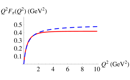
It is also instructive to use Eq. (43) to substitute in terms of . This gives
| (68) |
the expression analytically coinciding with our result obtained in Ref. Grigoryan:2007wn within the framework of the AdS/QCD model of Refs. Erlich:2005qh ; DaRold:2005zs .
This outcome has very basic reasons. Namely, the large- behavior of the form factor is determined, first, by the large- form of the bulk-to-boundary propagator (which coincides with its free-field version in any model) and, second, by the value of the pion wave function (or ) at the origin. The latter also determines in both holographic models, which results in the same analytic result for the large- limit of when it is expressed in terms of . However, as we already discussed in Ref. Grigoryan:2007wn , if we take the experimental value MeV, Eq. (68) gives the value that is well above Jefferson Lab’s experimental points. In this sense, the expression (67) for the limit of in terms of is numerically more successful than Eq. (68). One may speculate that since the pion form factor in our calculation is given by the ratio of the 3-point function term (which is proportional to ) to the 2-point function term (which is proportional to ), the overall error of the model in the value of is cancelled, and the remaining expression for in terms of correctly reflects information about the pion size.
From the form factor expression (III.2) and the decomposition of over the -channel bound states, one can extract the coupling:
| (69) | ||||
Here we took into account the correct normalization of currents, giving a factor of . From this result it follows that numerically . Taking we obtain . The experimental value is . The numbers obtained in Models A and B of Ref. Erlich:2005qh are and respectively.
IV Anomaly
IV.1 Chern-Simons action
Since the Chern-Simons/Wess-Zumino-Witten term for gauge/global group is vanishing, we need to extend the flavor symmetry to , so that the fields are written as
| (70) |
In order not to confuse the hats on the fields with the hats on the gauge fields in the axial gauge, we will assign hats only to the former and omit these for the latter.
Extending the holographic dictionary, the 4D isosinglet vector current will correspond to
| (71) |
where is the abelian part of the field. We also remind that the third component of the isovector current corresponds to
| (72) |
Note that the EM current of QCD is defined as
| (73) |
It has both isovector (“-type”) and isosinglet (“-type”) terms.
The part of the 5D CS action, in the axial gauge is
where . In the holographic model (cf. Domokos:2007kt ), the CS term is
| (74) |
where and .
After long, but straightforward calculations, we get
| (75) | ||||
Integrating the second term by parts with respect to and taking appropriate care on the IR boundary gives
| (76) |
Recall that and, in this model, it has the meaning of the pion “wave function”.
IV.2 Anomalous Form Factor
In QCD, the form factor is defined by
| (77) | ||||
where is the pion momentum, are the momenta of photons, and .
Varying gives the 3-point function:
| (78) |
with
| (79) |
where is the non-normalizable mode, see Eq. (61). It satisfies EOM given by Eq. (30), and is normalized by for . Note that deriving the result for we used the fact that both isoscalar and isosinglet vector mesons are described by the same EOM and b.c.
QCD axial anomaly requires: . Indeed, in the present extended holographic model, we get:
| (80) |
This result for the anomalous form factor is very similar to that obtained in our paper Grigoryan:2008up , where we worked out a CS extension of the hard-wall model of Refs. Erlich:2005qh ; DaRold:2005zs . However, in the present model, we do not have a bulk field dual to the chiral condensate operator of QCD, and, moreover, we do not need to add a counterterm on the IR boundary to reproduce the correct normalization of the anomalous form factor.
When only one of the photons is virtual, , while another is real, , we have
| (81) |
It is easy to notice that this expression for coincides with the expression (64) for , i.e., the anomalous form factor in this model coincides with the pion EM form factor!
The slope of the anomalous form factor defined as
| (82) |
in the present model is given by
| (83) |
Numerically, we have (compare with the recent result in Ref. Pomarol:2008aa ). This number is not very far from the central values of two last experiments, Farzanpay:1992pz , MeijerDrees:1992qb , but the experimental errors are rather large. An earlier experiment Fonvieille:1989kj produced , a result whose central value has opposite sign and much larger absolute magnitude. In the spacelike region, the data are available only for the values GeV2 (CELLO Behrend:1990sr ) and GeV2 (CLEO Gronberg:1997fj ) which cannot be treated as very small. The CELLO collaboration Behrend:1990sr gives the value that is very close to our result. To settle the uncertainty of the timelike data (and also on its own grounds), it would be interesting to have data on the slope from the spacelike region of very small , which may be obtained by modification of the PRIMEX experiment primex at JLab.
IV.3 coupling
Substituting and into Eq. (76), we obtain
Here, we introduced the dimensionful pion field . This lagrangian is similar to that obtained in the hidden local symmetries approach Fujiwara:1984mp (see also a review Meissner:1987ge ). Thus, we may write that
| (84) | ||||
The numerical value of this coupling is (for ). The value of this coupling and especially its sign have important phenomenological implementations, see e.g. Ref. Nakayama:2006ps . However, one cannot directly measure this coupling constant, since the decay is energetically forbidden.
IV.4 Large- behavior
Equation (81) formally gives prediction for the form factor at all , and it is interesting to compare it with the monopole fit (fitted value is MeV) of CLEO data Gronberg:1997fj which extend to GeV2. The comparison demonstrating a rather good agreement is shown in Fig. 2, where the value is taken for the AdS/QCD curve.
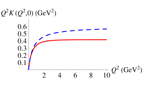
One may also consider the general case of large virtualities, when and , with being a fixed parameter, and large. In this limit, the bulk-to-boundary propagators in Eq. (79) may be substituted by their free-field version . Since exponentially decreases for large , the -integral is dominated by small , and Eq. (79) converts into
| (85) | ||||
Using Eq. (43) to substitute the overall factor by , we obtain exactly the result derived in our earlier paper Grigoryan:2007wn within the extension of the hard-wall model of Refs. Erlich:2005qh ; DaRold:2005zs . This coincidence in analytic form is analogous to that observed in the pion electromagnetic form factor case. Indeed, the large- asymptotics is determined by the large- behavior of the bulk-to-boundary propagators, which is the same (free-field-like) in all the models, and by the value of the pion wave function at the origin, which is fixed by the pion decay constant. Numerically, however, the results of the present model based on (85) would depend on whether one takes the experimental value for or substitutes by . Again, the situation is the same as in the pion EM form factor case.
V Summary and conclusions
Working within the framework of the holographic dual model of QCD proposed by Hirn and Sanz, we study form factors of the pion, namely, the electromagnetic form factor of charged pions and the anomalous form factor of the neutral pion. In order to calculate the latter, we extend the Hirn-Sanz model by incorporating the Chern-Simons term into the original 5D action.
Due to a simple form of the pion “wave function” , the pion form factor can be written in explicit analytic form involving the modified Bessel function. This analytic expression gives a simple formula for the pion charge radius in terms of the hard-wall scale , which is the only parameter of the model fixed by the value of the -meson mass. Written as a function of and , the prediction of the present model is in a good agreement with experiment both for low and high values. We also established that the low energy coupling constant in the present model is in better agreement with experiment than the result of the hard-wall AdS/QCD model of Ref. Erlich:2005qh .
We extended the model of Hirn and Sanz by adding the Chern-Simons term and demonstrated that such an extension correctly reproduces QCD anomaly. There was no need to introduce an IR counterterm which was required in our previous paper Grigoryan:2008up , where we worked in the framework of the hard-wall AdS/QCD model of Refs. Erlich:2005qh ; DaRold:2005zs . We also observed that the anomalous pion form factor with one real and one virtual photon with momentum transfer in the present model is given by exactly the same analytic expression as the form factor of the charged pion evaluated for the same . This outcome may be partially due to a very simple form of the pion wave function.
We calculated the -slope of the anomalous form factor predicted by the present model, which was considered earlier in our paper Grigoryan:2008up and was also recently discussed in the Ref. Pomarol:2008aa . In addition, we calculated the value of the coupling, which is important for phenomenological considerations. Finally, we showed that in the large -region we reproduce the same results as in case of the hard-wall model of Refs. Erlich:2005qh ; DaRold:2005zs .
It is encouraging to establish that such a simple model containing just one free parameter, the confinement scale , produces the results which are in good agreement with experimental findings. Moreover, most of the important expressions can be represented analytically without making any approximations. One can think that the role of the scalar field in the hard-wall AdS/QCD model is now played by the appropriate b.c. on the IR. However, with this simplicity, we loose information about the chiral condensate and the dependence of the observables on it. This dependence was studied in our earlier papers Grigoryan:2007wn ; Grigoryan:2008up .
VI Acknowledgments
H.R.G. would like to thank J. Erlich, C. Carone, T. S. Lee and C. D. Roberts for valuable comments, and A. W. Thomas for support at Jefferson Laboratory.
We thank the organizers of the program “From Strings to Things: String Theory Methods in QCD and Hadron Physics” at the Institute for Nuclear Theory at the University of Washington for support during this program, the participation in which stimulated the completion of this work.
This paper is authored by Jefferson Science Associates, LLC under U.S. DOE Contract No. DE-AC05-06OR23177. The U.S. Government retains a non-exclusive, paid-up, irrevocable, world-wide license to publish or reproduce this manuscript for U.S. Government purposes.
References
- (1) J. M. Maldacena, Adv. Theor. Math. Phys. 2, 231 (1998) [Int. J. Theor. Phys. 38, 1113 (1999)]; S. S. Gubser, I. R. Klebanov and A. M. Polyakov, Phys. Lett. B 428, 105 (1998); E. Witten, Adv. Theor. Math. Phys. 2, 253 (1998)
- (2) J. Polchinski and M. J. Strassler, Phys. Rev. Lett. 88, 031601 (2002); JHEP 0305, 012 (2003)
- (3) H. Boschi-Filho and N. R. F. Braga, JHEP 0305, 009 (2003); Eur. Phys. J. C 32, 529 (2004)
- (4) S. J. Brodsky and G. F. de Téramond, Phys. Lett. B 582, 211 (2004); G. F. de Teramond and S. J. Brodsky, Phys. Rev. Lett. 94, 201601 (2005)
- (5) T. Sakai and S. Sugimoto, Prog. Theor. Phys. 113, 843 (2005); 114, 1083 (2006)
- (6) J. Erlich, E. Katz, D. T. Son and M. A. Stephanov, Phys. Rev. Lett. 95, 261602 (2005)
- (7) J. Erlich, G. D. Kribs and I. Low, Phys. Rev. D 73, 096001 (2006)
- (8) L. Da Rold and A. Pomarol, Nucl. Phys. B 721, 79 (2005); JHEP 0601, 157 (2006)
- (9) A. Karch, E. Katz, D. T. Son and M. A. Stephanov, Phys. Rev. D 74, 015005 (2006)
- (10) C. Csaki and M. Reece, JHEP 0705, 062 (2007)
- (11) T. Hambye, B. Hassanain, J. March-Russell and M. Schvellinger, Phys. Rev. D 74, 026003 (2006); ibid. 76, 125017 (2007).
- (12) J. Hirn and V. Sanz, JHEP 0512, 030 (2005);
- (13) J. Hirn, N. Rius and V. Sanz, Phys. Rev. D 73, 085005 (2006)
- (14) K. Ghoroku, N. Maru, M. Tachibana and M. Yahiro, Phys. Lett. B 633, 602 (2006)
- (15) S. J. Brodsky and G. F. de Teramond, Phys. Rev. Lett. 96, 201601 (2006)
- (16) N. Evans, A. Tedder and T. Waterson, JHEP 0701, 058 (2007)
- (17) R. Casero, E. Kiritsis and A. Paredes, Nucl. Phys. B 787, 98 (2007).
- (18) U. Gursoy and E. Kiritsis, JHEP 0802, 032 (2008).
- (19) U. Gursoy, E. Kiritsis and F. Nitti, JHEP 0802, 019 (2008).
- (20) O. Bergman, S. Seki and J. Sonnenschein, JHEP 0712, 037 (2007).
- (21) J. Erdmenger, K. Ghoroku and I. Kirsch, JHEP 0709, 111 (2007).
- (22) J. Erdmenger, N. Evans, I. Kirsch and E. Threlfall, Eur. Phys. J. A 35, 81 (2008).
- (23) A. Dhar and P. Nag, JHEP 0801, 055 (2008).
- (24) H. R. Grigoryan and A. V. Radyushkin, Phys. Lett. B 650, 421 (2007).
- (25) H. R. Grigoryan, Phys. Lett. B 662, 158 (2008)
- (26) H. R. Grigoryan and A. V. Radyushkin, Phys. Rev. D 76, 115007 (2007).
- (27) H. R. Grigoryan and A. V. Radyushkin, Phys. Rev. D 77, 115024 (2008).
- (28) D. T. Son and M. A. Stephanov, Phys. Rev. D 69, 065020 (2004).
- (29) C. Vafa and E. Witten, Nucl. Phys. B 234, 173 (1984).
- (30) S. K. Domokos and J. A. Harvey, Phys. Rev. Lett. 99, 141602 (2007).
- (31) H. J. Kwee and R. F. Lebed, Phys. Rev. D 77, 115007 (2008); JHEP 0801, 027 (2008).
- (32) A. Pomarol and A. Wulzer, arXiv:0807.0316 [hep-ph].
- (33) S. Eidelman et al. [Particle Data Group], Phys. Lett. B 592, 1 (2004)
- (34) T. Fujiwara, T. Kugo, H. Terao, S. Uehara and K. Yamawaki, Prog. Theor. Phys. 73, 926 (1985).
- (35) U. G. Meissner, Phys. Rept. 161, 213 (1988).
- (36) K. Nakayama, Y. Oh, J. Haidenbauer and T. S. Lee, Phys. Lett. B 648, 351 (2007).
- (37) H. J. Behrend et al. [CELLO Collaboration], Z. Phys. C 49, 401 (1991).
- (38) J. Gronberg et al. [CLEO Collaboration], Phys. Rev. D 57, 33 (1998)
- (39) F. Farzanpay et al., Phys. Lett. B 278, 413 (1992).
- (40) R. Meijer Drees et al. [SINDRUM-I Collaboration], Phys. Rev. D 45, 1439 (1992).
- (41) H. Fonvieille et al., Phys. Lett. B 233, 65 (1989).
- (42) A. Gasparian, et al. “A Precision Measurement of the Neutral Pion Lifetime via the Primakoff Effect”, JLab proposal PR-02-103, http://www.jlab.org/primex/