Abstract:

We present the determination of a set of parton distributions of the nucleon, at next-to-leading order, from a global set of deep-inelastic scattering data: NNPDF1.0. The determination is based on a Monte Carlo approach, with neural networks used as unbiased interpolants. This method, previously discussed by us and applied to a determination of the nonsinglet quark distribution, is designed to provide a faithful and statistically sound representation of the uncertainty on parton distributions. We discuss our dataset, its statistical features, and its Monte Carlo representation. We summarize the technique used to solve the evolution equations and its benchmarking, and the method used to compute physical observables. We discuss the parametrization and fitting of neural networks, and the algorithm used to determine the optimal fit. We finally present our set of parton distributions. We discuss its statistical properties, test for its stability upon various modifications of the fitting procedure, and compare it to other recent parton sets. We use it to compute the benchmark W and Z cross sections at the LHC. We discuss issues of delivery and interfacing to commonly used packages such as LHAPDF.

1 Introduction

1.1 Determination of parton distributions

The determination of parton distributions has gone through various phases which mirror the evolution of theoretical and phenomenological understanding of the theory of strong interactions. At a very early stage [1, 2, 3, 4, 5, 6], parton distributions were determined through a combination of general physical principles (as embodied in sum rules), model assumptions and the first crude experimental information coming from Bjorken scaling and its violation. These determinations were semi-quantitative at best, and they were aimed at showing the compatibility of the data with the partonic interpretation of hard processes. The parton sets were used to compare the observed scaling violations with those predicted by perturbative QCD [2, 3, 4, 5, 6], thereby leading to first tests of the theory of strong interactions. These early investigations met with such success that the parton set of Buras and Gaemers [7] is sometimes still used today [8].

As the accuracy of the data and the confidence in perturbative QCD improved, the gluon distribution was extracted from scaling violations [9], and first parton sets based on consistent global fits were performed [10, 11]. Despite the availability of next-to-leading order evolution tools [12], these analyses were performed at leading order, which was accurate enough for these sets to be widely used for phenomenology in the ensuing decade.

However, thanks to a second generation of high–precision deep-inelastic scattering [13] and hadron collider [14] experiments, QCD gradually evolved towards being viewed as precision physics — an integral part of the standard model. This required an approach to parton determination based on next-to-leading order theory (in order to have perturbative uncertainties under control), and also based on fairly wide “global” sets of data of a varied nature, in order to minimize as much as possible the role of theoretical prejudice in the determination of the shape of the parton distributions at the initial scale [15, 16, 17, 18].

Next-to-leading order parton sets evolved into standard analysis tools and were constantly updated throughout the ensuing decade [19]. In particular, the wealth of data from the HERA collider [20] led to a considerable increase in the size of the kinematic region over which parton distributions could be determined, along with a substantial improvement in accuracy, especially in the determination of quantities which are sensitive to scaling violations. Accumulated knowledge eventually led to parton sets (such as as the CTEQ5 [21] and MRST2001 [22] sets) very likely to have an accuracy comparable to that of next-to-leading order QCD computation, adequate for the determination of most hard processes at collider energies. These parton sets differ in many technical details, but are rooted in a similar approach: a parton parametrization is assumed, based on the functional form $f(x)\sim x^{\alpha}(1-x)^{\beta}$ (used since the earliest investigations [1]), and its parameters are then tuned so that the various computed observables fit the experimental data.

With parton distributions now a tool for precision physics, it becomes important to be able to assess accurately the uncertainty on any given parton set. This need was recognized at a relatively early stage, and in fact the parton set of Ref. [16] included error parton sets along with average ones. However, providing error estimates which can be relied upon raises many subtle issues, the most obvious of which is the need for a full treatment of correlated uncertainties of the underlying data. In the absence of a full understanding of the problem, the only way of estimating the uncertainty related to the parton distribution was to compare results obtained with several parton sets, an especially unsatisfactory procedure given that many possible sources of systematic bias are likely to be common to several parton determinations.

Some first determinations of parton distributions with uncertainties were obtained by only fitting to restricted data sets (typically from a subset of deep-inelastic experiments), but retaining all the information on the correlated uncertainties in the underlying data, and propagating it through the fitting procedure [23, 24, 25]. The need for a systematic approach which could lead to parton distributions with reliable uncertainty estimation was stressed in the seminal papers Ref. [26, 27], where an entirely different approach to parton determination was suggested, based on Bayesian inference combined with a Monte Carlo approach. While the approach of Ref. [27] was never fully implemented, the need for parton sets with uncertainties is now generally recognized, and there are currently at least three sets of parton distributions with uncertainties available, maintained by the CTEQ [28, 29, 30, 31, 32], MRST-MSTW [33, 34, 35, 36] and Alekhin [37, 38, 39, 40] groups.

Parton distributions with uncertainties [28, 33, 40] have now become standard. Nevertheless, many of the problems raised in Refs. [26, 27] are still only partly solved. In particular, benchmark comparisons performed between some of these sets [41] have shown that the uncertainties that come with them are not easily interpreted in a statistical sense, in that they are to a significant amount determined or constrained by theoretical or phenomenological expectations. Indeed, whereas uncertainty bands for parton determinations based on restricted data sets [40] are obtained by using standard error propagation of one–sigma contours, those for global fits which include a large variety of data [33, 28] are obtained on the basis of a tolerance [28], determined by studying the compatibility of the data with each other and with the underlying theory. The effect of this tolerance is equivalent to multiplying experimental errors by a factor between four and six.

This state of affairs might be the inevitable consequences of incompatibilities between data and, possibly, of inadequacy of the theory used to describe them. Be that as it may, the standard parton determination method based on fitting a particular functional form does not seem to be sufficiently flexible to ascertain whether this is the case: in the absence of a term of comparison, it is hard to tell to which extent the current difficulties are due to an intrinsic limitation of the methodology.

An altogether new approach was proposed in Ref. [42]. The general aim of this approach is to determine objectively both the value and the uncertainty of a function (or set of functions) from a discrete set of many independent (and possibly incompatible) experimental measurements. Its viability was originally demonstrated by using it to provide a determination of the structure function $F_{2}(x,Q^{2})$ of the proton and neutron from its direct measurement at around 600 points, each by two independent experiments [42]. The method was then used in Ref. [43] to provide a state-of-the art determination of the same structure function for the proton, by combining almost 2000 different measurements in 13 different data sets, thereby addressing issues of data incompatibility. Finally, in Ref. [44] it was used to provide the determination of a single parton distribution (the nonsinglet quark distribution), thereby addressing the issue of determining a quantity which is not measured directly, but rather related through theory to an experimental observable. In the present paper, we use this method for the construction of a first parton set from deep-inelastic data: we determine five parton distributions from around 3000 measurements in 25 different data sets.

1.2 The NNPDF approach

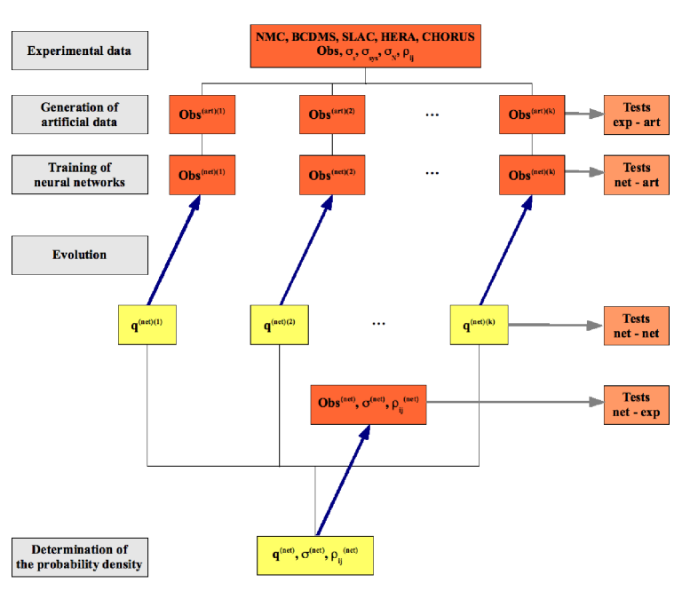
Figure 1: Schematic representation of the NNPDF approach.

The approach adopted here for the determination of parton distributions is based on a combination of a Monte Carlo method with the use of neural networks as basic interpolating functions. The general idea is twofold: first, problems related to the possibility of non-gaussian errors and nontrivial error propagation are best addressed through the use of a representation whereby central values are obtained from a Monte Carlo sample as averages, uncertainties as standard deviations, and so forth. Second, problems which require the reconstruction of a function through its discrete sampling, without making assumptions on its functional form, are best addressed using neural networks as unbiased interpolants. The combination of these two techniques works well in situations where data are partly inconsistent, in that neural networks are well suited to the separation of a smooth signal from background fluctuations, while the Monte Carlo handles the fluctuations themselves.

The strategy is summarized in Figure 1, and it involves two stages. In the first stage, one generates a Monte Carlo ensemble of replicas of the original data. This ensemble is generated with the probability distribution of the data, and it is large enough that the statistical properties of the data are reproduced to the desired accuracy. In practice, most data are given with multigaussian probability distributions of statistical and systematic errors, described by a covariance matrix and a normalization error, and in such cases this is the distribution that will be used to generate the pseudodata. However, any other probability distribution can be used if and when required by the experimental data. Each element in the Monte Carlo set is a replica of the experimental data: each replica contains as many data points as are originally available. The ensemble contains all the available experimental information, which can be reproduced by performing statistical operations on the replicas which form the ensemble. That indeed the given ensemble has the desired statistical features can be verified by means of standard tests, such as comparison of quantities calculated from it with the original properties of the data: this is denoted in Fig. 1 as “tests exp-art”, namely, the comparison of experimental and artificial data.

In the second stage, a set of parton distributions is constructed from each replica of the data. Each parton distribution function (PDF) at a given scale is parametrized by an individual neural network: the neural network is just an especially convenient functional form of parton parametrization, used in place of the usual functional forms. Physical observables are computed from parton distributions in the usual way. One first chooses a basis set of initial parton distributions, typically smaller than the maximal set of twelve quarks and antiquarks plus one gluon — here we use a set of five independent parton distributions. One then evolves from the initial scale to the scale at which data are available by using standard QCD evolution equations, and physical observables are computed by convoluting the evolved parton distributions with hard partonic cross sections. The best fit set of parton distribution is finally determined by comparing the theoretical computation of the observable for a given PDF set with their replica experimental values. The experimental values will of course be different in each replica — they will fluctuate according to their distribution in the Monte Carlo ensemble — and the best fit PDFs will be accordingly different for each replica. The ensemble of these best fit PDFs, which contains as many elements as the set of replicas of the data that were generated, is the final result of the parton determination.

The way in which the best fit set of PDFs is determined from each data replica is especially important. A first obvious requirement is that the best fit be independent of any assumptions made about the parton parametrization. This requirement is met by adopting a redundant parametrization: the size of the neural networks used, i.e. the number of parameters used to parametrize them, is much larger than the minimum required in order to reproduce the data. This redundancy may be checked a posteriori, by verifying that results are independent of the size and architecture of the neural network.

A more subtle issue is that of establishing how the best fit is to be determined. A first possible answer might be to determine the best fit as the absolute minimum of the $\chi^{2}$ (i.e. absolute maximum of the likelihood) of the comparison between theory and data for a given replica. As already pointed out in Ref. [42], however, this procedure does not produce the optimal fit for quantities with some built–in smoothness, such as physical cross sections. Indeed, even for fully compatible data, independent measurements of the same quantity at the same point will fluctuate within the uncertainty of the measurement. If fitted by maximum likelihood, such independent measurements will automatically be combined into their weighted average [45]. However, assume now that two independent measurements are performed of the same observable, but measured at very close values of the underlying kinematic variables: for example the structure function $F(x,Q^{2})$ at the same $Q^{2}$ and two different but close values $x$. Then a fit which goes through the central values of both measurements might be possible, but in the limit in which the two measurements are performed at infinitesimally close points this would correspond to a discontinuous behaviour of the observable, which is surely unphysical. This problem is exacerbated in the case of incompatible measurements.

It was thus suggested already in Ref. [42] that the best fit should be characterized by a value of the $\chi^{2}$ which is not as small as possible, but rather equal to the value expected on the basis of the fluctuations of the data. In order to determine this value, a strategy was developed in Ref. [44], based on the cross-validation method used quite generally in neural network studies [46]. Namely, for each replica, the data are divided randomly into a training set and a validation set. The fit is then performed on the data in the training set, and the $\chi^{2}$ computed from data in both sets is monitored. Minimization is stopped when the $\chi^{2}$ in the validation set (not used for fitting) stops decreasing. The method is made possible by the availability of a very large and mostly compatible set of data, and it guarantees that the best fit does not attempt to reproduce random fluctuations of the data. The method also handles incompatible data, by automatically tolerating fluctuations in the data even when they are larger than the nominal uncertainty, whenever fitting these fluctuations would not lead to an improvement of the global quality of the fit. This analysis is denoted as “tests net-art” in Fig. 1, namely, the comparison of neural net to the previously generated artificial data.

An important feature of this approach is that many issues of parton determination can be now addressed using standard statistical tools. For example, the stability of results upon a change of parametrization can be verified by computing the distance between results in units of their standard deviation. An advantage of the Monte Carlo approach is that it is no more difficult to do this for uncertainties, correlation coefficients or even more indirect quantities, than it is for values of physical observables. Likewise, it is possible to verify that fits performed by removing data from the set have wider error bands but remain compatible within these enlarged uncertainties, and so forth. The reliability of the results, in particular for the uncertainties on the PDFs, can thus be assessed directly. This assessment is denoted as “tests net-net” in Fig. 1.

Of course, it is also possible to perform the standard tests based on the comparison of the final fit prediction with the original input data set. The most fundamental of these is the comparison to the data (and the computation of the corresponding $\chi^{2}$) for the best fit obtained by averaging results over all neural nets in the final sample. These tests are denoted as “tests net-exp” in Fig. 1: the comparison of the final set of neural nest to the starting experimental data set.

The implementation of this approach for the parton fit presented here follows the principles and techniques presented in Ref. [44]. In this paper we present the adaptations which are needed in order to go from the determination of a single parton distribution to that of a full set. We also present in detail the features and results of this specific PDF determination, NNPDF1.0, and in particular the results of the tests discussed above.

The paper is organized as follows. In Section 2 we present the data which will be used in our determination, along with their main statistical features, and the kinematic cuts that we have applied to them, and the results of tests to verify that the Monte Carlo sample provides a faithful representation of these data. In Section 3 we summarize the method we use to solve evolution equations (already introduced in Ref. [44] in the nonsinglet case), provide results from its benchmarking, describe the specific basis of PDFs we use, and discuss the computation of physical observables with the inclusion target-mass corrections. Full details of the hard kernels used to construct the physical observables are given in Appendix A. In Section 4 we turn to the neural network parametrization and minimization: we summarize the structure of neural networks used, the weighted genetic algorithm which has been employed to train them, and the stopping algorithm used to determine the best fit along the lines discussed above (already introduced in Ref. [44]) and present the parameter settings and specific features used in the current fits. In Section 5 we discuss in detail our results: we discuss the general statistical features of our reference parton set, and present the individual PDFs and their correlations; we discuss the results of various stability tests related to the architecture of neural network (size and choice of the preprocessing function) and the dataset (kinematic cuts and reduced datasets); we study theoretical uncertainties, specifically higher order corrections and the choice of value of the strong coupling; finally we present results computed using our dataset both for some of the physical observables entering the fit (such as structure functions and reduced cross sections) and for benchmark LHC observables (the W and Z total cross sections). Useful formulae for the determination of uncertainties on physical observables using various different PDF sets are summarized in Appendix B. An outlook on future developments is provided in Section 6.

2 Experimental data and Monte Carlo generation

The determination of PDFs presented in this work is based on a comprehensive set of experimental data from deep-inelastic scattering (DIS) with various lepton beams and nucleon targets. We choose a purely DIS data set for this first fit because of the known general consistency of DIS data. We include both proton data and neutron data from nuclear targets in order to be able to disentangle isospin triplet and isospin singlet contribution. We also include charged current scattering data from charged lepton beams and neutrino scattering data in order to be able to disentangle the quark and antiquark distributions. Because of the limitations due to only fitting DIS data, we will take a basis of five independent parton distributions, namely the two light flavours and antiflavours and the gluon, as we discuss below in Sect. 3.6. Further constraints on PDFs could be obtained from various other experiments, in particular from hadron-hadron scattering. The inclusion of these data in our fit is conceptually straightforward, and is left to forthcoming publications. We shall first present the general features of the data we use, then discuss the construction of the covariance matrix, provide definitions of relevant observables and finally present the generation and testing of the Monte Carlo sample of pseudodata.

2.1 The data set

The data sets used in this study are listed in Table 1, and their kinematic coverage is shown in Fig. 2. They can be summarized as follows.

We use the data for proton and deuteron structure functions $F_{2}^{p,d}$ determined in fixed-target experiments by the BCDMS [47, 48] and NMC [49, 50] collaborations, which were already included in our previous analysis of the nonsinglet quark distribution in Ref. [44]. They provide the most accurate and up-to-date information on the valence region of parton distributions. They are supplemented with data on the structure functions from SLAC [51] which, though rather older and less precise, improve the kinematic coverage in the large $x$ region. Compared to previous studies by our collaboration, we now use the ratio $F_{2}^{d}/F_{2}^{p}$ whenever data for this observable are available, thereby benefitting from cancellations in the correlated systematic uncertainties. Altogether these data cover the middle- to large-$x$ and smaller $Q^{2}$ region of the kinematical range, corresponding to the lower-right corner in Fig. 2.

Collider experiments have explored a larger kinematical range in great detail. Neutral and charged current reduced cross sections from the H1 [52, 53, 54, 55] and ZEUS [56, 57, 58, 59, 60, 61] collaborations are used in the current fit. As shown in Fig. 2 these data sets yield informations in a much wider region of the $(x,Q^{2})$ plane, in both the small-$x$ and the large-$Q^{2}$ directions. We also include the data for $F_{L}$ that have recently appeared in Ref. [62]. This is a rather small data set, but it provides the only direct measurement of $F_{L}$. We refer to Refs. [42, 43, 44] for additional informations on all the data sets that were used in our earlier studies.

In order to be able to control the valence–sea (or quark–antiquark) separation, in this fit we also include neutrino DIS data. Specifically, we use the large, up-to-date, and consistent set of neutrino and antineutrino scattering data by the CHORUS collaboration [63]. These data have a similar kinematic coverage to the fixed target charged lepton DIS data.

The main features of our data sets are summarized in Table 1, where we show the beam, target and observable, the number of data points, the kinematic range, the size of uncertainties averaged over the data points. The observable chosen is generally that which is closest to the experimental measurement and minimizes the pre-analysis by the experimental collaboration: in particular we have used the reduced cross section for all collider and neutrino data sets. The various systematics and their correlations are treated according to the information provided by the experimental collaborations themselves (see Section 2 in Ref. [42] for a detailed description of NMC and BCDMS data, Table 1 in Ref. [64] for ZEUS data, Table 2 in Ref. [55] for H1 data,Ref. [65] for CHORUS data).

In Table 1 we distinguish between “Experiments”, defined as groups of data that are not correlated to each other, and “Sets” within an experiment, which are correlated with each other. They correspond to measurements of different observables in the same experiment, or measurements of the same observables in different years which retain some correlated systematics. This distinction will be important in the minimization strategy, discussed in Section 4.2 below.

Experiment	Set	$N_{\rm dat}$	$x_{\rm min}$	$x_{\rm max}$	$Q^{2}_{\rm min}$	$Q^{2}_{\rm max}$	$\sigma_{\rm tot}$ (%)	$F$	Ref.
SLAC
	SLACp	211 (47)	.07000	.85000	0.6	29.	3.6	$F_{2}^{p}$	[51]
	SLACd	211 (47)	.07000	.85000	0.6	29.	3.2	$F_{2}^{d}$	[51]
BCDMS
	BCDMSp	351 (333)	.07000	.75000	7.5	230.	5.5	$F_{2}^{p}$	[47]
	BCDMSd	254 (248)	.07000	.75000	8.8	230.	6.6	$F_{2}^{d}$	[48]
NMC		288 (245)	.00350	.47450	0.8	61.	5.0	$F_{2}^{p}$	[50]
NMC-pd		260 (153)	.00150	.67500	0.2	99.	2.1	$F_{2}^{d}/F_{2}^{p}$	[49]
ZEUS
	Z97lowQ2	80	.00006	.03200	2.7	27.	4.9	$\tilde{\sigma}^{NC,e^{+}}$	[56]
	Z97NC	160	.00080	.65000	35.0	20000.	7.7	$\tilde{\sigma}^{NC,e^{+}}$	[56]
	Z97CC	29	.01500	.42000	280.0	17000.	34.2	$\tilde{\sigma}^{CC,e^{+}}$	[57]
	Z02NC	92	.00500	.65000	200.0	30000.	13.2	$\tilde{\sigma}^{NC,e^{-}}$	[58]
	Z02CC	26	.01500	.42000	280.0	30000.	40.2	$\tilde{\sigma}^{CC,e^{-}}$	[59]
	Z03NC	90	.00500	.65000	200.0	30000.	9.1	$\tilde{\sigma}^{NC,e^{+}}$	[60]
	Z03CC	30	.00800	.42000	280.0	17000.	31.0	$\tilde{\sigma}^{CC,e^{+}}$	[61]
H1
	H197mb	67 (55)	.00003	.02000	1.5	12.	4.9	$\tilde{\sigma}^{NC,e^{+}}$	[52]
	H197lowQ2	80	.00016	.20000	12.0	150.	4.2	$\tilde{\sigma}^{NC,e^{+}}$	[52]
	H197NC	130	.00320	.65000	150.0	30000.	13.3	$\tilde{\sigma}^{NC,e^{+}}$	[53]
	H197CC	25	.01300	.40000	300.0	15000.	29.8	$\tilde{\sigma}^{CC,e^{+}}$	[53]
	H199NC	126	.00320	.65000	150.0	30000.	15.5	$\tilde{\sigma}^{NC,e^{-}}$	[54]
	H199CC	28	.01300	.40000	300.0	15000.	27.6	$\tilde{\sigma}^{CC,e^{-}}$	[54]
	H199NChy	13	.00130	.01050	100.0	800.	9.2	$\tilde{\sigma}^{NC,e^{-}}$	[55]
	H100NC	147	.00131	.65000	100.0	30000.	10.4	$\tilde{\sigma}^{NC,e^{+}}$	[55]
	H100CC	28	.01300	.40000	300.0	15000.	21.8	$\tilde{\sigma}^{CC,e^{+}}$	[55]
CHORUS
	CHORUS$\nu$	607 (471)	.02000	.65000	0.3	95.	11.2	$\tilde{\sigma}^{\nu}$	[63]
	CHORUS$\bar{\nu}$	607 (471)	.02000	.65000	0.3	95.	18.7	$\tilde{\sigma}^{\bar{\nu}}$	[63]
FLH108		8	.00028	.00360	12.0	90.	69.2	$F_{L}$	[62]
Total		3948 (3161)

Table 1: The experiments included in the present analysis divided in the respective data sets. We show the number of points before (after) applying kinematic cuts, the kinematic range, the average total uncertainty and the measured observable. Different sets within an experiment are correlated with each other, but data from different experiments are not.

2.2 Uncertainties and correlations

The covariance matrix for each experiment can be computed from knowledge of statistical, systematic and normalization uncertainties:

$${\rm cov}_{pq}=\left(\sum_{l=1}^{N_{c}}\sigma_{p,l}\sigma_{q,l}+\sum_{n=1}^{N_{a}}\sigma_{p,n}\sigma_{q,n}+\sum_{n=1}^{N_{r}}\sigma_{p,n}\sigma_{q,n}+\delta_{pq}\sigma_{p,s}^{2}\right)F_{p,I}F_{q,J}\ ,$$ (1)

where $p$ and $q$ run over the experimental points, $F_{I,p}=F_{I}(x_{p},Q_{p}^{2})$ and $F_{J,q}=F_{J}(x_{q},Q_{q}^{2})$ are the measured central values for the observables $I$ and $J$, and the various uncertainties, given as relative values, are: $\sigma_{p,l}$, the $N_{c}$ correlated systematic uncertainties; $\sigma_{p,n}$, the $N_{a}$ ($N_{r}$) absolute (relative) normalization uncertainties; $\sigma_{p,s}$ the statistical uncertainty.

The correlation matrix is defined as

$$\rho_{pq}={{{\rm cov}_{pq}}\over{\sigma_{p,\mathrm{tot}}\sigma_{q,\mathrm{tot}}F_{p,I}F_{q,J}}}\ ,$$ (2)

where the total uncertainty $\sigma_{p,{\rm tot}}$ for the $p$-th point is given by

$$\sigma_{p,\mathrm{tot}}=\sqrt{\sigma_{p,s}^{2}+\sigma_{p,c}^{2}+\sigma_{p,N}^{2}}\,,$$ (3)

the total correlated uncertainty $\sigma_{p,c}$ is the sum of all correlated systematics

$$\sigma_{p,c}^{2}=\sum_{l=1}^{N_{c}}\sigma_{p,l}^{2}\,,$$ (4)

and the total normalization uncertainty is

$$\sigma_{p,N}^{2}=\sum_{n=1}^{N_{a}}\sigma_{p,n}^{2}+\sum_{n=1}^{N_{r}}\left(\hbox{${{1}\over{2}}$}\sigma_{p,n}\right)^{2}.$$ (5)

The factor of one half in the relative normalization uncertainties comes from the first order expansion of Eq. (14) below.

The $N_{u}$ uncorrelated systematic uncertainties quoted for HERA data sets are combined with the statistical uncertainty according to

$$\sigma_{p,s}^{2}=\sigma_{p,stat}^{2}+\sum_{k=1}^{N_{u}}\sigma_{p,k}^{2}.$$ (6)

Asymmetric uncertainties quoted for some ZEUS data sets in Refs. [58, 59, 60, 61] are symmetrized as described in Section 2 of Ref. [43] and references therein. For the case of SLAC data the single systematic uncertainty is taken to be fully correlated for all the data points.

2.3 Observables and kinematic cuts

The deep-inelastic observables used in our fit are either structure functions or reduced cross sections. The neutral current deep-inelastic scattering cross section involving a generic charged lepton $\ell^{\pm}$ is defined as

$${{d^{2}\sigma^{\rm NC,\ell^{\pm}}}\over{dxdQ^{2}}}(x,y,Q^{2})={{2\pi\alpha^{2}}\over{xQ^{4}}}\left[Y_{+}F_{2}^{NC}(x,Q^{2})\mp Y_{-}xF_{3}^{NC}(x,Q^{2})-y^{2}F_{L}^{NC}(x,Q^{2})\right]\ ,$$ (7)

where

$$Y_{\pm}=1\pm(1-y)^{2}.$$ (8)

In the case of NMC, BCDMS, and SLAC data, we use the quoted value for the structure function $F_{2}(x,Q^{2})$. For ZEUS and H1 data, we use the quoted reduced cross section defined as

$$\widetilde{\sigma}^{\rm NC,e^{\pm}}(x,y,Q^{2})=\left[{{2\pi\alpha^{2}}\over{xQ^{4}}}Y_{+}\right]^{-1}{{d^{2}\sigma^{\rm NC,e^{\pm}}}\over{dxdQ^{2}}}(x,y,Q^{2})\,.$$ (9)

For charged current deep-inelastic scattering, the measured double differential cross section in the case of unpolarized beams is given by

$${{d^{2}\sigma^{\rm CC,e^{\pm}}}\over{dxdQ^{2}}}(x,y,Q^{2}) = {{G_{F}^{2}}\over{4\pi x}}\left({{M_{W}^{2}}\over{M_{W}^{2}+Q^{2}}}\right)^{2}$$

$$\times {{1}\over{2}}\left[Y_{+}F_{2}^{CC,e^{\pm}}(x,Q^{2})\mp Y_{-}xF_{3}^{CC,e^{\pm}}(x,Q^{2})-y^{2}F_{L}^{CC,e^{\pm}}(x,Q^{2})\right]\,.$$

As in the neutral current case we use the reduced cross section defined as

$$\widetilde{\sigma}^{\rm CC,e^{\pm}}(x,y,Q^{2})=\left[{{G_{F}^{2}}\over{4\pi x}}\left({{M_{W}^{2}}\over{M_{W}^{2}+Q^{2}}}\right)^{2}\right]^{-1}{{d^{2}\sigma^{\rm CC,e^{\pm}}}\over{dxdQ^{2}}}(x,y,Q^{2})\,.$$ (11)

In the case of CHORUS data, we use the neutrino-nucleon reduced cross section, which in the single $W$-exchange approximation, can be written as

$$\tilde{\sigma}^{\nu(\bar{\nu})}(x,y,Q^{2}) = {{1}\over{E_{\nu}}}{{d^{2}\sigma^{\nu(\bar{\nu})}}\over{dx\,dy}}(x,y,Q^{2})$$

$$= {{G_{F}^{2}M_{N}}\over{2\pi(1+Q^{2}/M_{W}^{2})^{2}}}\left[\left(Y_{+}-{{2M^{2}_{N}x^{2}y^{2}}\over{Q^{2}}}\right)F_{2}^{\nu(\bar{\nu})}\pm\,Y_{-}\,xF_{3}^{\nu(\bar{\nu})}-y^{2}F_{L}^{\nu(\bar{\nu})}\right].$$

For all nuclear targets, namely NMC, BCDMS and SLAC deuteron data and CHORUS heavy nuclei (mostly lead with a small admixture of iron and other materials), no nuclear corrections are applied.

In order to keep higher–twist corrections under control, only data with $Q^{2}>2\,{\rm GeV^{2}}$ and $W^{2}>12.5\,{\rm GeV^{2}}$ are retained. The changes, if any, in the number of data points after kinematic cuts for each set are reported in Table 1 between parenthesis. The experimental data actually used in the present analysis are summarized in Fig. 2. Since the kinematic cuts we use are not too conservative, we will supplement our fit with target mass corrections, as discussed in Section 3.8.

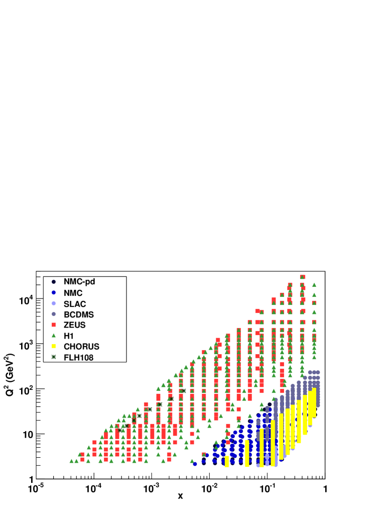
Figure 2: Experimental data in the $(x,Q^{2})$ plane used in the present analysis after kinematic cuts.

2.4 Generation of the pseudo-data sample

Error propagation from experimental data to the fit is handled by a Monte Carlo sampling of the probability distribution defined by data. The statistical sample is obtained by generating $N_{\rm rep}$ artificial replicas of data points following a multi-gaussian distribution centered on each data point with the variance given by the experimental uncertainty. More precisely, given a data point $F_{I,p}^{\rm(exp)}\equiv F_{I}(x_{p},Q^{2}_{p})$ we generate $k=1,\ldots,N_{\mathrm{rep}}$ artificial points $F_{I,p}^{(\mathrm{art})(k)}$ as follows

$$F_{I,p}^{(\mathrm{art})(k)}=S_{p,N}^{(k)}F_{I,p}^{\rm(\mathrm{exp})}\left(1+\sum_{l=1}^{N_{c}}r_{p,l}^{(k)}\sigma_{p,l}+r_{p}^{(k)}\sigma_{p,s}\right)\ ,\ k=1,\ldots,N_{\mathrm{rep}}\ ,$$ (13)

where

$$S_{p,N}^{(k)}=\prod_{n=1}^{N_{a}}\left(1+r_{p,n}^{(k)}\sigma_{p,n}\right)\prod_{n=1}^{N_{r}}\sqrt{1+r_{p,n}^{(k)}\sigma_{p,n}}.$$ (14)

The variables $r_{p,l}^{(k)},r_{p}^{(k)},r_{p,n}^{(k)}$ are all univariate gaussian random numbers that generate fluctuations of the artificial data around the central value given by the experiments. For each replica $k$, if two experimental points $p$ and $p^{\prime}$ have correlated systematic uncertainties, then $r^{(k)}_{p,l}=r^{(k)}_{p^{\prime},l}$, i.e. the fluctuations due to the correlated systematic uncertainties are the same for both points. A similar condition on $r^{(k)}_{p,n}$ ensures that correlations between normalization uncertainties are properly taken into account.

Experiment	NMC	NMC-pd	SLAC	BCDMS
$\left\langle PE\left[\left\langle F^{\rm(art)}\right\rangle_{\rm rep}\right]\right\rangle_{\rm dat}$	9.0 $\cdot 10^{-5}$	1.8 $\cdot 10^{-5}$	3.1 $\cdot 10^{-4}$	1.3 $\cdot 10^{-3}$
$r\left[F^{\rm(art)}\right]$	1.000	1.000	1.000	1.000
$\left\langle PE\left[\left\langle\sigma^{\rm(art)}\right\rangle_{\rm rep}\right]\right\rangle_{\rm dat}$	1.5 $\cdot 10^{-3}$	4.2 $\cdot 10^{-3}$	3.1 $\cdot 10^{-3}$	4.0 $\cdot 10^{-3}$
$\left\langle\sigma^{\rm(exp)}\right\rangle_{\rm dat}$	0.0147	0.0170	0.0104	0.0698
$\left\langle\sigma^{\rm(art)}\right\rangle_{\rm dat}$	0.0146	0.0171	0.0104	0.0692
$r\left[\sigma^{\rm(art)}\right]$	1.000	0.998	0.998	0.999
$\left\langle\rho^{\rm(exp)}\right\rangle_{\rm dat}$	0.033	0.165	0.312	0.470
$\left\langle\rho^{\rm(art)}\right\rangle_{\rm dat}$	0.033	0.176	0.311	0.463
$r\left[\rho^{\rm(art)}\right]$	0.963	0.988	0.987	0.994
$\left\langle{\rm cov}^{\rm(exp)}\right\rangle_{\rm dat}$	6.52 $\cdot 10^{-6}$	4.39 $\cdot 10^{-5}$	3.07 $\cdot 10^{-5}$	2.90 $\cdot 10^{-5}$
$\left\langle{\rm cov}^{\rm(art)}\right\rangle_{\rm dat}$	6.78 $\cdot 10^{-6}$	4.73 $\cdot 10^{-5}$	3.03 $\cdot 10^{-5}$	2.82 $\cdot 10^{-5}$
$r\left[{\rm cov}^{\rm(art)}\right]$	0.989	0.984	0.988	0.999
Experiment	ZEUS	H1	CHORUS	FLH108	Total
$\left\langle PE\left[\left\langle F^{\rm(art)}\right\rangle_{\rm rep}\right]\right\rangle_{\rm dat}$	8.5 $\cdot 10^{-4}$	1.1 $\cdot 10^{-4}$	1.8 $\cdot 10^{-3}$	1.3 $\cdot 10^{-2}$	7.1 $\cdot 10^{-5}$
$r\left[F^{\rm(art)}\right]$	1.000	1.000	1.000	1.000	0.980
$\left\langle PE\left[\left\langle\sigma^{\rm(art)}\right\rangle_{\rm rep}\right]\right\rangle_{\rm dat}$	9.6 $\cdot 10^{-3}$	4.2 $\cdot 10^{-3}$	1.8 $\cdot 10^{-2}$	6.1 $\cdot 10^{-4}$	3.0 $\cdot 10^{-3}$
$\left\langle\sigma^{\rm(exp)}\right\rangle_{\rm dat}$	0.0607	0.0472	0.1088	0.1744	0.0556
$\left\langle\sigma^{\rm(art)}\right\rangle_{\rm dat}$	0.0603	0.0472	0.1109	0.1756	0.0562
$r\left[\sigma^{\rm(art)}\right]$	1.000	1.000	0.998	0.999	0.980
$\left\langle\rho^{\rm(exp)}\right\rangle_{\rm dat}$	0.079	0.027	0.094	0.650	0.145
$\left\langle\rho^{\rm(art)}\right\rangle_{\rm dat}$	0.082	0.028	0.096	0.657	0.146
$r\left[\rho^{\rm(art)}\right]$	0.982	0.952	0.998	0.996	0.996
$\left\langle{\rm cov}^{\rm(exp)}\right\rangle_{\rm dat}$	1.53 $\cdot 10^{-4}$	4.93 $\cdot 10^{-5}$	2.16 $\cdot 10^{-3}$	2.03 $\cdot 10^{-2}$	1.07 $\cdot 10^{-3}$
$\left\langle{\rm cov}^{\rm(art)}\right\rangle_{\rm dat}$	1.57 $\cdot 10^{-4}$	5.03 $\cdot 10^{-5}$	2.31 $\cdot 10^{-3}$	2.11 $\cdot 10^{-2}$	1.01 $\cdot 10^{-3}$
$r\left[{\rm cov}^{\rm(art)}\right]$	0.996	0.987	0.998	0.998	0.997

Table 2: Statistical estimators for the Monte Carlo artificial data generation with $N_{\mathrm{rep}}=1000$. The definition of the statistical estimators is given in Appendix B of [44].

The treatment of normalization uncertainties needs some care: as is well known, including normalization uncertainties in the covariance matrix would lead to a fit that is systematically biased to lie below the data [66]. Rather, normalization uncertainties are included by rescaling all uncertainties, i.e. by constructing for each replica a modified covariance matrix:

$${\overline{\rm cov}^{(k)}}_{pq}=\left(\sum_{l=1}^{N_{c}}{\overline{\sigma}^{(k)}}_{p,l}{\overline{\sigma}^{(k)}}_{q,l}+\delta_{pq}\left({\overline{\sigma}^{(k)}}_{p,s}\right)^{2}\right)F_{I,p}F_{J,q}\ ,$$ (15)

with the statistical uncertainties $\sigma_{p,s}$ and each systematic uncertainty $\sigma_{p,l}$ being rescaled according to

$$\overline{\sigma}_{p,s}^{(k)}=S_{p,N}^{(k)}\sigma_{p,s}\,,\qquad\qquad\overline{\sigma}_{p,l}^{(k)}=S_{p,N}^{(k)}\sigma_{p,l}\,,\qquad l=1,\ldots,N_{c}\,.$$ (16)

It can be readily seen that:

$${\overline{\rm cov}^{(k)}}_{pq}={\overline{\rm cov}^{(\mathrm{exp})}}_{pq}S_{p,N}^{(k)}S_{q,N}^{(k)}\,,$$ (17)

and therefore the experimental correlation matrix without normalization uncertainties needs to be evaluated only once, while ${\overline{\rm cov}^{(k)}}_{pq}$ is obtained by multiplying by the normalization factors $S_{p,N}^{(k)}$ and $S_{q,N}^{(k)}$ for each replica. If within an experiment all the sets have only a common global normalization uncertainty, the rescaling is an overall multiplicative factor. The covariance matrix Eq. (15) is that which is used in order to perform a fit to the $k$-th data replica.

Appropriate statistical estimators have been devised in Ref. [44] in order to quantify the accuracy of the statistical sampling obtained from a given ensemble of replicas. We refer the reader to Appendix B of Ref. [44] for a detailed explanation of the meaning of these statistical estimators. Using these estimators, we have verified that a Monte Carlo sample of pseudo-data with $N_{\mathrm{rep}}=1000$ is sufficient to reproduce the mean values, the variances, and the correlations of experimental data with a 1% accuracy for all the experiments. Results for the estimators computed from a sample of $N_{\mathrm{rep}}=1000$ replicas are shown in Table 2. This set of Monte Carlo replicas will be used in the rest of this paper.

3 From parton distributions to physical observables

In this section we provide all the technical details for the calculation in perturbation theory of deep–inelastic observables from a set of initial PDFs. First, we briefly review the strategy for the solution of QCD evolution equations in terms of pre-computable perturbative hard kernels $K_{Ij}((x,\alpha_{s}(Q^{2}),\alpha_{s}(Q_{0}^{2}))$, originally introduced in Ref. [44]. Then we review the calculation of the DGLAP evolution factors $\Gamma_{ij}(x,\alpha_{s}(Q^{2}),\alpha_{s}(Q_{0}^{2}))$ using Mellin space techniques, including our prescription for heavy quarks, and give details of their benchmarking. Next, we turn to the particular choice of basis for the input PDFs. Finally, we describe the calculation of physical observables by combining evolved PDFs with the hard coefficient functions (including their target mass corrections) and the procedure for obtaining the hard kernels $K_{Ij}((x,\alpha_{s}(Q^{2}),\alpha_{s}(Q_{0}^{2}))$ for deep inelastic observables.

3.1 Leading-twist factorization and evolution

The perturbative computation of physical observables involves first evolving the PDFs up to the scale of the measurement, and then their convolution with a hard cross-section to give the observable. Here this is done following the strategy of Ref. [44], whereby evolution kernels are pre-computed, and then convoluted with parton distributions. This separates the numerical computation of the solutions to evolution equations from the computation of input parton distributions. The advantage of this is that each of the two computations can be optimized separately from a numerical point of view: in particular, we can thus use a Mellin-space approach to solve evolution equations, but adopt $x$-space parametrization of PDFs. Also, evolution kernels can thus be pre-computed, benchmarked, and stored for future use during the fitting procedure.

The basic ideas behind this technique were discussed in [44]. The extension from the nonsinglet structure function, with only one PDF, to a number of different deep inelastic structure functions and reduced cross-sections, expressed in terms of several singlet and nonsinglet PDFs, is in principle straightforward, but in practice complicated by a number of subtleties which will be discussed as they arise.

Deep inelastic observables $F_{I}(x,Q^{2})$ (which may be structure functions or reduced cross-sections) may always be expressed at leading twist as a convolution of parton distributions $f_{j}(x,Q^{2})$ and hard coefficient functions $C_{Ij}(x,\alpha_{s}(Q^{2}))$, computed in perturbation theory:

$$F_{I}(x,Q^{2})=\sum_{j}C_{Ij}(x,\alpha_{s}(Q^{2}))\otimes f_{j}(x,Q^{2}),\,$$ (18)

where $\otimes$ denotes the convolution

$$f(x)\otimes g(x)\equiv\int_{x}^{1}{{dy}\over{y}}f(y)g\left({{x}\over{y}}\right),\,$$ (19)

and the indices $I$ and $j$ run over observables and parton distribution functions respectively. The scale dependence of the parton distribution functions is in turn given by the renormalisation group, or DGLAP equations

$$Q^{2}{{\partial}\over{\partial Q^{2}}}f_{i}(x,Q^{2})=\sum_{j}P_{ij}(x,\alpha_{s}(Q^{2}))\otimes f_{j}(x,Q^{2}),\,$$ (20)

where $P_{ij}$ are the Altarelli-Parisi splitting functions, also calculable in perturbation theory.

The solution of these coupled integro-differential equations may be written as

$$f_{i}(x,Q^{2})=\sum_{j}\Gamma_{ij}(x,\alpha_{s},\alpha_{s}^{0})\otimes f_{j}(x,Q_{0}^{2}),\,$$ (21)

where $f_{j}(x,Q_{0}^{2})$ are the input PDFs, to be determined empirically, $\Gamma_{ij}(x,\alpha_{s},\alpha_{s}^{0})$ are the evolution factors, and we use the shorthand notation

$$\alpha_{s}\equiv\alpha_{s}(Q^{2}),\qquad\alpha_{s}^{0}\equiv\alpha_{s}(Q_{0}^{2}).$$ (22)

The evolution factors also satisfy evolution equations:

$$Q^{2}{{\partial}\over{\partial Q^{2}}}\Gamma_{ij}(x,\alpha_{s},\alpha_{s}^{0})=\sum_{k}P_{ik}(x,\alpha_{s})\otimes\Gamma_{kj}(x,\alpha_{s},\alpha_{s}^{0}),\,$$ (23)

with boundary conditions $\Gamma_{ij}(x,\alpha_{s}^{0},\alpha_{s}^{0})=\delta_{ij}\delta(1-x)$.

Substituting Eq. (21) into Eq. (18)

$$F_{I}(x,Q^{2}) = \sum_{jk}C_{Ij}(x,\alpha_{s})\otimes\Gamma_{jk}(x,\alpha_{s},\alpha_{s}^{0})\otimes f_{k}(x,Q_{0}^{2})\,$$ (24)

$$= \sum_{j}K_{Ij}(x,\alpha_{s},\alpha_{s}^{0})\otimes f_{j}(x,Q_{0}^{2}),\,$$

where the hard kernel

$$K_{Ij}(x,\alpha_{s},\alpha_{s}^{0})=\sum_{k}C_{Ik}(x,\alpha_{s})\otimes\Gamma_{kj}(x,\alpha_{s},\alpha_{s}^{0}),\,$$ (25)

may be computed in perturbation theory.

Performing many nested convolutions is numerically rather time consuming. However the hard kernels Eq. (25) are independent of the particular set of input PDFs adopted, and may thus be calculated once and for all at the beginning of the computation, interpolated, and stored. Determining the physical observables given by a given set of input PDFs then involves the evaluation of only the one set of convolutions Eq. (24), which is relatively fast, these being reducible to simple sums.

3.2 Solving the evolution equations

The QCD evolution equations are most easily solved using Mellin moments [16, 67, 68], since then all the convolutions become simple products, and the equations can be solved in closed form. The problem is thus reduced to the computation of the single Mellin inversion integral. Specifically, we define

$$\Gamma_{ij}(N,\alpha_{s},\alpha_{s}^{0})\equiv\int_{0}^{1}\!dx\,x^{N-1}\Gamma_{ij}(x,\alpha_{s},\alpha_{s}^{0})\ ,$$ (26)

where by slight abuse of notation we denote the function and its transform with the same symbol. Equation (23) becomes

$$Q^{2}{{\partial}\over{\partial Q^{2}}}\Gamma_{ij}(N,\alpha_{s},\alpha_{s}^{0})=\sum_{k}\gamma_{ik}(N,\alpha_{s})\,\Gamma_{kj}(N,\alpha_{s},\alpha_{s}^{0})\ ,$$ (27)

where the anomalous dimensions $\gamma_{ij}(N,\alpha_{s})$ are the Mellin moments of the splitting functions. Expanding perturbatively in powers of $\alpha_{s}$

$$\gamma_{ij}(N,\alpha_{s})=\alpha_{s}\gamma^{(0)}_{ij}(N)+\alpha_{s}^{2}\gamma^{(1)}_{ij}(N)+\cdots,$$ (28)

where the dots denote higher order contributions. The anomalous dimensions are known at LO, NLO [69, 70, 71, 72, 73, 74] and NNLO [75, 76].

Since all the dependence on $Q^{2}$ of the anomalous dimension is through the running coupling $\alpha_{s}(Q^{2})$, and

$${{d\alpha_{s}}\over{d\ln Q^{2}}}=\beta(\alpha_{s})=-\alpha_{s}^{2}\beta_{0}-\alpha_{s}^{3}\beta_{1}+\cdots\,,$$ (29)

we may in turn write Eq. (27) as a differential equation in $\alpha_{s}$:

$${{\partial}\over{\partial\ln\alpha_{s}}}\Gamma_{ij}(N,\alpha_{s},\alpha_{s}^{0})=-\sum_{k}R_{ik}(N,\alpha_{s})\Gamma_{kj}(N,\alpha_{s},\alpha_{s}^{0}).\,$$ (30)

The matrix $R_{ij}\equiv({\bf R})_{ij}$ has the perturbative expansion

$${\bf R}(N,\alpha_{s})={\bf R}^{(0)}(N)+\alpha_{s}{\bf R}^{(1)}(N)+\cdots,$$ (31)

where in terms of the expansion Eq. (28) of the anomalous dimension matrix $\gamma_{ij}\equiv({\boldsymbol{\gamma}})_{ij}$

$${\bf R}^{(0)}(N)\equiv{{\boldsymbol{\gamma}^{(0)}(N)}\over{\beta_{0}}},\qquad{\bf R}^{(k)}(N)\equiv{{\boldsymbol{\gamma}^{(k)}(N)}\over{\beta_{0}}}-\sum_{i=1}^{k}{{\beta_{i}}\over{\beta_{0}}}{\bf R}^{(k-i)}(N).\,$$ (32)

Note that Eq. (27) truncated at NLO, that is with Eq. (28) and Eq. (29) truncated after the first two terms, is not equivalent to the naive truncation of Eq. (31) after two terms, but rather to the complete series with

$${\bf R}^{(0)}(N)\equiv\boldsymbol{\gamma}^{(0)}(N)/\beta_{0},\qquad{\bf R}^{(k)}(N)\equiv-b_{1}{\bf R}^{(k-1)}(N),$$ (33)

where $b_{1}\equiv\beta_{1}/\beta_{0}$.

The complete matrix of anomalous dimensions $\boldsymbol{\gamma}$, and thus the matrices ${\bf R}$ are in fact almost completely diagonal: all the flavour nonsinglet and valence quark distributions evolve multiplicatively, and only the singlet quark and gluon actually mix. Thus we only need to solve Eq. (30) for one by one and two by two matrices.

Consider first the simplest case of the evolution of flavour nonsinglet and valence quark distributions: the evolution factor then satisfies the simple first order equation

$${{\partial}\over{\partial\ln\alpha_{s}}}\Gamma_{\rm NS}(N,\alpha_{s},\alpha_{s}^{0})=-R_{\rm NS}(N,\alpha_{s})\Gamma_{\rm NS}(N,\alpha_{s},\alpha_{s}^{0}).\,$$ (34)

At LO the solution is trivial:

$$\Gamma_{\rm NS,LO}(N,\alpha_{s},\alpha_{s}^{0})=\left({{\alpha_{s}}\over{\alpha_{s}^{0}}}\right)^{-R^{(0)}_{\rm NS}},$$ (35)

while at NLO we need to work a little harder: using Eq. (33) one finds

$$\Gamma_{\rm NS,NLO}(N,\alpha_{s},\alpha_{s}^{0})=\exp\left\{-{{R^{(1)}_{\rm NS}}\over{b_{1}}}\ln\left({{1+b_{1}\alpha_{s}}\over{1+b_{1}\alpha_{s}^{0}}}\right)\right\}\left({{\alpha_{s}}\over{\alpha_{s}^{0}}}\right)^{-R^{(0)}_{\rm NS}}.$$ (36)

This exact solution is equivalent up to subleading terms to the linearized solution

$$\Gamma^{\rm lin}_{\rm NS,NLO}(N,\alpha_{s},\alpha_{s}^{0})=\left(1-R^{(1)_{\rm NS}}(\alpha_{s}-\alpha_{s}^{0})\right)\left({{\alpha_{s}}\over{\alpha_{s}^{0}}}\right)^{-R^{(0)}_{\rm NS}},$$ (37)

which is in turn the exact solution to Eq. (34) with $R_{\rm NS}=R^{(0)}_{\rm NS}+\alpha_{s}R^{(1)}_{\rm NS}$.

Turning finally to the singlet sector, we need to solve Eq. (30) when ${\bf R}$ are two by two matrices, corresponding to coupled singlet quarks and gluons:

$${{\partial}\over{\partial\ln\alpha_{s}}}{\bf\Gamma}_{\rm S}(N,\alpha_{s},\alpha_{s}^{0})=-{\bf R}_{\rm S}(N,\alpha_{s}){\bf\Gamma}_{\rm S}(N,\alpha_{s},\alpha_{s}^{0}).\,$$ (38)

At LO we can proceed by diagonalization:

$${\bf\Gamma}_{\rm S,LO}(N,\alpha_{s},\alpha_{s}^{0})\equiv{\bf L}(N,\alpha_{s},\alpha_{s}^{0})={\bf e}_{+}(N)\left({{\alpha_{s}}\over{\alpha_{s}^{0}}}\right)^{-\lambda_{+}(N)}+{\bf e}_{-}(N)\left({{\alpha_{s}}\over{\alpha_{s}^{0}}}\right)^{-\lambda_{-}(N)},$$ (39)

where

$$\lambda_{\pm}(N)={{1}\over{2\beta_{0}}}\left[\gamma^{(0)}_{qq}(N)+\gamma^{(0)}_{gg}(N)\pm\sqrt{\left(\gamma^{(0)}_{qq}(N)-\gamma^{(0)}_{gg}(N)\right)^{2}+4\gamma^{(0)}_{qg}(N)\gamma^{(0)}_{gq}(N)}\right],$$ (40)

are the eigenvalues of the two by two matrix ${\bf R}_{\rm S}^{(0)}(N)$ of singlet anomalous dimensions, and

$${\bf e}_{\pm}(N)=\pm{{1}\over{\lambda_{+}(N)-\lambda_{-}(N)}}({\bf R}_{\rm S}^{(0)}(N)-\lambda_{\mp}(N){\bf I})\,,$$ (41)

are the corresponding projectors.

The full NLO solution is more complicated, and must be developed recursively as a perturbative expansion around the LO solution ${\bf L}(N,as,\alpha_{s}^{0})$: writing

$${\bf\Gamma}_{\rm S,NLO}(N,\alpha_{s},\alpha_{s}^{0})\equiv{\bf U}(N,\alpha_{s}){\bf L}(N,\alpha_{s},\alpha_{s}^{0}){\bf U}(N,\alpha_{s}^{0})^{-1},$$ (42)

where ${\bf U}(N,\alpha_{s})$ has the expansion

$${\bf U}(N,\alpha_{s})={\bf 1}+\alpha_{s}{\bf U}^{(1)}(N)+\alpha_{s}^{2}{\bf U}^{(2)}(N)+\cdots,$$ (43)

solves Eq. (30) provided

$${\bf U}^{(k)}={{{\bf e}_{-}\widetilde{{\bf R}}^{(k)}{\bf e}_{+}}\over{\lambda_{+}-\lambda_{-}-k}}+{{{\bf e}_{+}\widetilde{{\bf R}}^{(k)}{\bf e}_{-}}\over{\lambda_{-}-\lambda_{+}-k}}-{{1}\over{k}}\left[{\bf e}_{+}\widetilde{{\bf R}}^{(k)}{\bf e}_{+}+{\bf e}_{-}\widetilde{{\bf R}}^{(k)}{\bf e}_{-}\right],$$ (44)

where

$$\widetilde{{\bf R}}^{(0)}={\bf R}_{\rm S}^{(0)},\qquad\widetilde{{\bf R}}^{(k)}={\bf R}_{\rm S}^{(k)}+\sum_{i=1}^{k-1}{\bf R}_{\rm S}^{(k-i)}{\bf U}^{(i)}\,.$$ (45)

By solving recursively Eqs. (44), (45) with the NLO approximation Eq. (33), the NLO evolution factor Eq. (33) can be computed. Just as in the nonsinglet case, the exact NLO solution may be linearized to give

$${\bf\Gamma}^{\rm lin}_{\rm S,NLO}(N,\alpha_{s},\alpha_{s}^{0})={\bf L}(N,\alpha_{s},\alpha_{s}^{0})+\alpha_{s}{\bf U}^{(1)}(N){\bf L}(N,\alpha_{s},\alpha_{s}^{0})-\alpha_{s}^{0}{\bf L}(N,\alpha_{s},\alpha_{s}^{0}){\bf U}^{(1)}(N),$$ (46)

which again is an exact solution to the truncated evolution equation, and equivalent to the full solution Eq. ((42)) up to subleading terms.

In what follows we will use the exact solutions Eq. (36) and Eq. (42) in order to be able to compare our results directly to those of $x$-space codes (see e.g. [77, 78]) which integrate the evolution equations numerically. However in the comparison to the data we choose the linearized solutions Eq. (37) and Eq. (46).

Generalization of the NLO solutions to NNLO and beyond is straightforward but tedious.

3.3 Calculating the evolved $x$-space PDFs

The $x$–space evolution factors are obtained by taking the inverse Mellin transforms of the solutions obtained in Eq. (36) and Eq. (42). For the nonsinglets

$$\Gamma_{\rm NS}(x,\alpha_{s},\alpha_{s}^{0})=\int_{C}{{dN}\over{2\pi i}}x^{-N}\Gamma_{\rm NS}(N,\alpha_{s},\alpha_{s}^{0}),$$ (47)

where $C$ is taken to be the Talbot contour described in ref.[44], which goes around the singularities at $N=0,-1,-2,\ldots$. For the singlets we use instead

$${\bf\Gamma}_{\rm S}(x,\alpha_{s},\alpha_{s}^{0})=\int_{C+1}{{dN}\over{2\pi i}}x^{-N}{\bf\Gamma}_{\rm S}(N,\alpha_{s},\alpha_{s}^{0})=x\,\int_{C}{{dN}\over{2\pi i}}x^{-N}{\bf\Gamma}_{\rm S}(N-1,\alpha_{s},\alpha_{s}^{0}),$$ (48)

since now the singularities are at $N=1,0,-1,\ldots$, i.e. displaced by one unit to the right. The contour integrals are evaluated using the Fixed Talbot algorithm [79].

However all splitting functions, except the off-diagonal entries of the singlet matrix, diverge when $x\to 1$; this implies that the evolution kernels $\Gamma(x,\alpha_{s},\alpha_{s}^{0})$ will likewise be divergent as $x\to 1$, and must thus be interpreted as distributions. Specifically, we define

$$\Gamma_{\rm NS}^{(+)}(x,\alpha_{s},\alpha_{s}^{0}) = \Gamma_{\rm NS}(x,\alpha_{s},\alpha_{s}^{0})-G_{NS}(\alpha_{s},\alpha_{s}^{0})\delta(1-x)\,,$$ (49)

$${\bf\Gamma}_{\rm S}^{(+)}(x,\alpha_{s},\alpha_{s}^{0}) = {\bf\Gamma}_{\rm S}(x,\alpha_{s},\alpha_{s}^{0})-{\bf G}_{S}(\alpha_{s},\alpha_{s}^{0})\,x^{-1}\delta(1-x)\,,$$ (50)

where

$$G_{\rm NS}(\alpha_{s},\alpha_{s}^{0}) = \int_{0}^{1}\!dx\,\Gamma_{\rm NS}(x,\alpha_{s},\alpha_{s}^{0})=\Gamma_{\rm NS}(N,\alpha_{s},\alpha_{s}^{0})|_{N=1},$$ (51)

$${\bf G}_{\rm S}(\alpha_{s},\alpha_{s}^{0}) = \int_{0}^{1}\!dx\,x\,{\bf\Gamma}_{\rm S}(x,\alpha_{s},\alpha_{s}^{0})={\bf\Gamma}_{\rm S}(N,\alpha_{s},\alpha_{s}^{0})|_{N=2},\,$$ (52)

are all finite constants. The convolutions Eq. (21) may then be evaluated as

$$f_{i}(x,Q^{2}) = G_{\rm NS}(\alpha_{s},\alpha_{s}^{0})f_{i}(x,Q_{0}^{2})+\int_{x}^{1}\!{{dy}\over{y}}\,\Gamma_{\rm NS}^{(+)}(y,\alpha_{s},\alpha_{s}^{0})f_{i}\left({{x}\over{y}},Q_{0}^{2}\right)$$ (53)

$$= \left(G_{\rm NS}(\alpha_{s},\alpha_{s}^{0})-\int_{0}^{x}\!dy\,\Gamma_{\rm NS}(y,\alpha_{s},\alpha_{s}^{0})\right)f_{i}(x,Q_{0}^{2})$$

$$\qquad+\int_{x}^{1}\!{{dy}\over{y}}\,\Gamma_{\rm NS}(y,\alpha_{s},\alpha_{s}^{0})\left(f_{i}\left({{x}\over{y}},Q_{0}^{2}\right)-yf_{i}(x,Q_{0}^{2}),\right).$$

for nonsinglet distributions $f_{i}$, and similarly

$${\bf f}_{\rm S}(x,Q^{2}) = {\bf G}_{\rm S}(\alpha_{s},\alpha_{s}^{0}){\bf f}_{\rm S}(x,Q_{0}^{2})+\int_{x}^{1}\!{{dy}\over{y}}\,{\bf\Gamma}_{\rm S}^{(+)}(y,\alpha_{s},\alpha_{s}^{0}){\bf f}_{\rm S}\left({{x}\over{y}},Q_{0}^{2}\right)$$ (54)

$$= \left({\bf G}_{\rm S}(\alpha_{s},\alpha_{s}^{0})-\int_{0}^{x}\!dy\,y{\bf\Gamma}_{\rm S}(y,\alpha_{s},\alpha_{s}^{0})\right){\bf f}_{\rm S}(x,Q_{0}^{2})$$

$$\qquad+\int_{x}^{1}\!{{dy}\over{y}}\,{\bf\Gamma}_{\rm S}(y,\alpha_{s},\alpha_{s}^{0})\left({\bf f}_{\rm S}\left({{x}\over{y}},Q_{0}^{2}\right)-y^{2}{\bf f}_{\rm S}(x,Q_{0}^{2})\right),$$

for singlet distributions ${\bf f}_{\rm S}$, where now all integrals converge and can be computed numerically, in practice using Gaussian integration as described in ref.[44].

3.4 Flavour decomposition and heavy quarks

The primary quantities $f_{j}$ in Eq. (20) may be thought of as the $2n_{f}$ quark and antiquark distributions $q_{i}$ and $\overline{q}_{i}$ and the gluon distribution $g$. The singlet quark distribution

$$\Sigma=\sum_{i=1}^{n_{f}}(q_{i}+\overline{q}_{i})\,,$$ (55)

and the gluon distribution mix under evolution, as in Eq. (54): a sensible basis is ${\bf f}_{\rm S}=(\Sigma,g)$. For the remaining $2n_{f}-1$ distributions we adopt a basis of charge conjugation eigenvectors which each evolve independently according to Eq. (53): a suitable such basis consists of the $n_{f}-1$ charge conjugation even nonsinglets

$$T_{3} = u^{+}-d^{+},$$

$$T_{8} = u^{+}+d^{+}-2s^{+},$$

$$T_{15} = u^{+}+d^{+}+s^{+}-3c^{+},$$

$$T_{24} = u^{+}+d^{+}+s^{+}+c^{+}-4b^{+},$$

$$T_{35} = u^{+}+d^{+}+s^{+}+c^{+}+b^{+}-5t^{+},$$ (56)

where $q_{i}^{\pm}=q_{i}\pm\overline{q}_{i}$, and $q_{i}=u,d,s,c,b,t$ are the various flavour distributions, which evolve with evolution factor $\Gamma_{\rm NS}^{+}$, and the $n_{f}$ charge conjugation odd valence distributions

$$V = u^{-}+d^{-}+s^{-}+c^{-}+b^{-}+t^{-},$$

$$V_{3} = u^{-}-d^{-},$$

$$V_{8} = u^{-}+d^{-}-2s^{-},$$

$$V_{15} = u^{-}+d^{-}+s^{-}-3c^{-},$$

$$V_{24} = u^{-}+d^{-}+s^{-}+c^{-}-4b^{-},$$

$$V_{35} = u^{-}+d^{-}+s^{-}+c^{-}+b^{-}-5t^{-},$$ (57)

the first of which (the singlet) evolves with evolution factor $\Gamma_{\rm NS}^{v}$, while the remainder evolve with evolution factor $\Gamma_{\rm NS}^{-}$. At LO all the quark anomalous dimensions are equal: $\gamma_{\rm NS}^{(0),+}=\gamma_{\rm NS}^{(0),-}=\gamma_{\rm NS}^{(0),v}=\gamma_{\rm S,qq}^{(0)}$, and thus at LO $\Gamma_{\rm NS}^{+}=\Gamma_{\rm NS}^{-}=\Gamma_{\rm NS}^{v}=\Gamma_{\rm S}^{qq}$. However at NLO $\gamma_{\rm NS}^{(1),-}=\gamma_{NS}^{(1),v}$, while all the others are different: beyond NLO all the anomalous dimensions, and thus evolution factors, are different from each other.

We regard the first three flavours $u$, $d$ and $s$ as “light”: together with the gluon we thus have seven parton distributions $g,\Sigma,V,T_{3},T_{8},V_{3},V_{8}$ which are intrinsically nonperturbative and are thus, at least in principle, to be determined empirically. The parametrization of these PDFs will be discussed in the next section. The remaining three flavours $c$,$b$ and $t$ are regarded as “heavy”: this means that we assume that the six parton distributions $T_{15},T_{24},T_{35},V_{15},V_{24},V_{35}$ have a component which may be computed perturbatively. Of course, it is in principle possible to also introduce nonperturbative (or “intrinsic”) contributions to these quantities.

In this paper we use the zero mass variable flavour number (ZM-VFN) scheme to incorporate the effects of the heavy quarks. In this, the simplest heavy quark scheme, the number of virtual flavours in the $\beta$ function and anomalous dimensions changes abruptly at the heavy quark thresholds: this means that while the PDFs are continuous, their scale dependence is discontinuous. Thus for example, when computing $\Gamma(N,\alpha_{s},\alpha_{s}^{0})$ for $Q^{2}>m_{b}^{2}$, we write

$$\Gamma(N,\alpha_{s},\alpha_{s}^{0})=\Gamma(N,\alpha_{s},\alpha_{s}^{b})\Gamma(N,\alpha_{s}^{b},\alpha_{s}^{0}),$$ (58)

where $\alpha_{s}^{b}\equiv\alpha_{s}(m_{b}^{2})$, and compute the two factors on the right hand side with $n_{f}=4$ and $n_{f}=5$ respectively. This scheme neglects terms above threshold which are proportional to powers of ${{m^{2}_{h}}\over{Q^{2}}}$, where $m_{h}$ is the mass of the heavy quark, thereby losing accuracy for scales close to the thresholds.

The heavy quark distributions themselves are assumed to be zero below threshold, and then generated radiatively above threshold. Consider for example the charm distribution. For simplicity we take $Q_{0}^{2}=m_{c}^{2}$. For $Q^{2}\leq m_{c}^{2}$, $c^{\pm}=0$, so $T_{15}=\Sigma$, $V_{15}=V$, while for $Q^{2}>m_{c}^{2}$, $T_{15}$ and $V_{15}$ evolve as nonsinglet distributions:

$$T_{15}(x,Q^{2}) = \Gamma_{\mathrm{NS}}^{+}(x,\alpha_{s},\alpha_{s}^{0})\otimes\Sigma(x,Q_{0}^{2}),$$ (59)

$$V_{15}(x,Q^{2}) = \Gamma_{\mathrm{NS}}^{-}(x,\alpha_{s},\alpha_{s}^{0})\otimes V(x,Q_{0}^{2}).$$ (60)

The difference between $T_{15}(x,Q^{2})$ and the quark singlet $\Sigma(x,Q^{2})$ for $m_{c}^{2}<Q^{2}<m_{b}^{2}$ gives the charm distribution $c^{+}$. Similarly $c^{-}$ is given by the difference between $V_{15}(x,Q^{2})$ and $V(x,Q^{2})$: however since at NLO $\Gamma_{\rm NS}^{-}=\Gamma_{NS}^{v}$, $V_{15}=V$ and $c=\bar{c}$.

For the $b$ distribution the situation is a little more complicated since now $m_{b}^{2}>Q_{0}^{2}$. Assuming now that $b^{\pm}=0$ for $Q^{2}<m_{b}^{2}$, we have for $Q^{2}>m_{b}^{2}$

$$T_{24}(x,Q^{2}) = \Gamma_{\mathrm{NS}}^{+}(x,\alpha_{s},\alpha_{s}^{b})\otimes\Sigma(x,m_{b}^{2})$$ (61)

$$= \Gamma_{\mathrm{NS}}^{+}(x,\alpha_{s},\alpha_{s}^{b})\otimes$$

$$\qquad\qquad\left(\Gamma_{\mathrm{S}}^{qq}(x,\alpha_{s}^{b},\alpha_{s}^{0})\otimes\Sigma(x,Q_{0}^{2})+\Gamma_{\mathrm{S}}^{qg}(x,\alpha_{s}^{b},\alpha_{s}^{0})\otimes g(x,Q_{0}^{2})\right).$$

It is thus convenient to define the evolution factors

$$\Gamma^{24,q}_{\mathrm{S}}(N,\alpha_{s},\alpha_{s}^{0}) = \Gamma_{\mathrm{NS}}^{+}(N,\alpha_{s},\alpha_{s}^{b})\Gamma_{\mathrm{S}}^{qq}(N,\alpha_{s}^{b},\alpha_{s}^{0}),$$ (62)

$$\Gamma^{24,g}_{\mathrm{S}}(N,\alpha_{s},\alpha_{s}^{0}) = \Gamma_{\mathrm{NS}}^{+}(N,\alpha_{s},\alpha_{s}^{b})\Gamma_{\mathrm{S}}^{qg}(N,\alpha_{s}^{b},\alpha_{s}^{0}).$$

Note that these are inverted and convoluted using the singlet formulae Eq. (48) and Eq. (54) since at least a part of the evolution is singlet. Below threshold, i.e. for $Q^{2}<m_{b}^{2}$, $\Gamma^{24,q}_{\mathrm{S}}=\Gamma^{qq}_{\mathrm{S}}$, $\Gamma^{24,g}_{\mathrm{S}}=\Gamma^{qg}_{\mathrm{S}}$. Similarly, for evolution of the valence contribution $V_{24}(x,Q^{2})$ it is convenient to define

$$\Gamma^{24}_{\mathrm{NS}}(N,\alpha_{s},\alpha_{s}^{0})=\Gamma_{\mathrm{NS}}^{-}(N,\alpha_{s},\alpha_{s}^{b})\Gamma_{\mathrm{NS}}^{v}(N,\alpha_{s}^{b},\alpha_{s}^{0}).$$ (63)

above threshold, with $\Gamma^{24}_{\mathrm{NS}}=\Gamma^{v}_{\mathrm{NS}}$ below. At NLO, for all $Q^{2}$, $\Gamma^{24}_{\mathrm{NS}}=\Gamma_{\mathrm{NS}}^{-}=\Gamma_{\mathrm{NS}}^{v}$, thus $V_{24}=V$ and $b=\bar{b}$.

Precisely similar considerations apply to the top distribution: for $Q^{2}>m_{t}^{2}$ we define

$$\Gamma_{\rm S}^{35,q}(N,\alpha_{s},\alpha_{s}^{0}) = \Gamma_{\mathrm{NS}}^{+}(N,\alpha_{s},\alpha_{s}^{t})\Gamma_{\rm S}^{qq}(N,\alpha_{s}^{t},\alpha_{s}^{0}),$$ (64)

$$\Gamma_{\rm S}^{35,g}(N,\alpha_{s},\alpha_{s}^{0}) = \Gamma_{\mathrm{NS}}^{+}(N,\alpha_{s},\alpha_{s}^{t})\Gamma_{\rm S}^{qg}(N,\alpha_{s}^{t},\alpha_{s}^{0}).$$

$$\Gamma_{\rm NS}^{35}(N,\alpha_{s},\alpha_{s}^{0}) = \Gamma_{\mathrm{NS}}^{-}(N,\alpha_{s},\alpha_{s}^{t})\Gamma_{\rm NS}^{v}(N,\alpha_{s}^{t},\alpha_{s}^{0}),$$ (65)

to give the evolution of $T_{35}(x,Q^{2})$ and $V_{35}(x,Q^{2})$. For $Q^{2}<m_{t}^{2}$ $\Gamma^{35,q}_{\mathrm{S}}=\Gamma^{qq}_{\mathrm{S}}$, $\Gamma^{35,g}_{\mathrm{S}}=\Gamma^{qg}_{\mathrm{S}}$, $\Gamma^{35}_{\mathrm{NS}}=\Gamma^{v}_{\mathrm{NS}}$, and at NLO for all $Q^{2}$, $\Gamma^{35}_{\mathrm{NS}}=\Gamma_{\mathrm{NS}}^{-}=\Gamma_{\mathrm{NS}}^{v}$, $V_{35}=V$ and $t=\bar{t}$. Note however that all the data we currently use to determine the PDFs are actually below the top threshold.

3.5 Practical implementation and benchmarks

The solution of the evolution equations through the determination of $x-$space evolution factors, Eqs. (53) and (54), is particularly efficient because of the universality of the evolution factor, i.e., its independence of the specific boundary condition which is being evolved. This means that the evolution factors can be pre-computed and stored, and then used during the process of parton fitting without having to recompute them each time [44].

During PDF fitting, a given PDF set must be evolved many times up to the fixed values of $(x,Q^{2})$ at which data are available. It can be seen that for each $(x,Q^{2})$ the numerical determination of the right–hand side of Eqs. (53,54) involves the evaluation of two contributions: the first requires the multiplication of the PDF by a (predetermined) constant $(G(\alpha_{s},\alpha_{s}^{0})-\int_{0}^{x}\!dy\,\Gamma(y,\alpha_{s},\alpha_{s}^{0}))$ while the second requires a convolution of the (predetermined) evolution factor $\Gamma(y,\alpha_{s},\alpha_{s}^{0})$ with the (subtracted) PDF, and thus the numerical evaluation of the integral over $y$. To perform this numerical integration we use $N_{\rm quad}-$point gaussian integration in each of the $2^{N_{\rm iter}+1}-1$ intervals in which the integration range $(x,1)$ of $y$ is divided. The total number of points used to perform the convolutions in $y$ of Eqs. (53) and (54) is then given by

$$N_{\rm pt}=N_{\rm quad}\left(2^{N_{\rm iter}+1}-1\right)\ ,$$ (66)

and we determine the values of $y$ accordingly, for each given value of $x$. We find that $N_{\rm quad}=4$ is precise enough for all applications, and we discuss below in detail the choice of $N_{\rm iter}$.

$x$	$\epsilon_{\rm rel}\left(u_{v}\right)$	$\epsilon_{\rm rel}\left(d_{v}\right)$	$\epsilon_{\rm rel}\left(\Sigma\right)$	$\epsilon_{\rm rel}\left(\bar{d}+\bar{u}\right)$	$\epsilon_{\rm rel}\left(s+\bar{s}\right)$	$\epsilon_{\rm rel}\left(g\right)$
$N_{\rm iter}=6$
$10^{-7}$	$2.2~{}10^{-5}$	$8.1~{}10^{-6}$	$4.9~{}10^{-6}$	$1.5~{}10^{-5}$	$1.2~{}10^{-6}$	$2.2~{}10^{-5}$
$10^{-6}$	$6.3~{}10^{-6}$	$3.2~{}10^{-6}$	$9.8~{}10^{-6}$	$1.1~{}10^{-5}$	$5.4~{}10^{-6}$	$3.0~{}10^{-6}$
$10^{-5}$	$1.8~{}10^{-5}$	$1.4~{}10^{-5}$	$8.3~{}10^{-6}$	$3.0~{}10^{-6}$	$3.6~{}10^{-6}$	$1.4~{}10^{-6}$
$10^{-4}$	$3.1~{}10^{-5}$	$1.6~{}10^{-5}$	$3.6~{}10^{-5}$	$4.3~{}10^{-5}$	$3.3~{}10^{-5}$	$3.2~{}10^{-5}$
$10^{-3}$	$1.8~{}10^{-6}$	$1.2~{}10^{-5}$	$5.9~{}10^{-6}$	$5.8~{}10^{-6}$	$8.9~{}10^{-6}$	$3.6~{}10^{-6}$
$10^{-2}$	$2.8~{}10^{-5}$	$1.5~{}10^{-5}$	$4.7~{}10^{-5}$	$4.3~{}10^{-5}$	$4.6~{}10^{-5}$	$8.2~{}10^{-5}$
$0.1$	$3.2~{}10^{-6}$	$1.3~{}10^{-5}$	$3.0~{}10^{-6}$	$9.4~{}10^{-6}$	$2.1~{}10^{-5}$	$5.1~{}10^{-7}$
$0.3$	$1.9~{}10^{-6}$	$2.4~{}10^{-5}$	$6.5~{}10^{-6}$	$1.0~{}10^{-5}$	$3.2~{}10^{-6}$	$2.6~{}10^{-6}$
$0.5$	$1.70~{}10^{-5}$	$1.3~{}10^{-5}$	$1.5~{}10^{-5}$	$1.3~{}10^{-5}$	$3.0~{}10^{-6}$	$3.5~{}10^{-6}$
$0.7$	$7.0~{}10^{-5}$	$8.0~{}10^{-6}$	$5.9~{}10^{-5}$	$8.9~{}10^{-6}$	$2.4~{}10^{-5}$	$9.9~{}10^{-6}$
$0.9$	$1.4~{}10^{-5}$	$6.2~{}10^{-6}$	$1.3~{}10^{-5}$	$7.4~{}10^{-4}$	$1.8~{}10^{-3}$	$5.1~{}10^{-5}$
$N_{\rm iter}=4$
$10^{-7}$	$4.2~{}10^{-2}$	$4.5~{}10^{-2}$	$5.1~{}10^{-2}$	$5.1~{}10^{-2}$	$5.1~{}10^{-2}$	$5.1~{}10^{-2}$
$10^{-6}$	$1.6~{}10^{-2}$	$1.8~{}10^{-2}$	$2.4~{}10^{-2}$	$2.3~{}10^{-2}$	$2.4~{}10^{-2}$	$2.5~{}10^{-2}$
$10^{-5}$	$4.9~{}10^{-3}$	$4.4~{}10^{-3}$	$8.7~{}10^{-3}$	$8.3~{}10^{-3}$	$8.7~{}10^{-3}$	$9.6~{}10^{-3}$
$10^{-4}$	$2.3~{}10^{-3}$	$2.2~{}10^{-3}$	$3.9~{}10^{-3}$	$3.7~{}10^{-3}$	$3.9~{}10^{-3}$	$4.4~{}10^{-3}$
$10^{-3}$	$1.1~{}10^{-3}$	$6.7~{}10^{-4}$	$3.5~{}10^{-3}$	$3.0~{}10^{-3}$	$3.4~{}10^{-3}$	$4.6~{}10^{-3}$
$10^{-2}$	$1.5~{}10^{-3}$	$8.5~{}10^{-4}$	$3.4~{}10^{-3}$	$2.7~{}10^{-3}$	$3.7~{}10^{-3}$	$5.5~{}10^{-3}$
0.1	$3.9~{}10^{-6}$	$1.3~{}10^{-5}$	$4.3~{}10^{-6}$	$1.1~{}10^{-5}$	$2.4~{}10^{-5}$	$1.0~{}10^{-4}$
0.3	$1.9~{}10^{-6}$	$2.6~{}10^{-5}$	$6.6~{}10^{-6}$	$1.610^{-5}$	$5.9~{}10^{-6}$	$7.1~{}10^{-7}$
0.5	$1.6~{}10^{-5}$	$1.1~{}10^{-5}$	$1.4~{}10^{-5}$	$2.0~{}10^{-5}$	$5.8~{}10^{-6}$	$3.3~{}10^{-5}$
0.7	$6.8~{}10^{-5}$	$1.2~{}10^{-5}$	$5.7~{}10^{-5}$	$6.5~{}10^{-6}$	$4.6~{}10^{-5}$	$3.4~{}10^{-5}$
0.9	$1.4~{}10^{-5}$	$5.1~{}10^{-5}$	$1.6~{}10^{-5}$	$6.4~{}10^{-4}$	$1.7~{}10^{-3}$	$1.2~{}10^{-4}$

Table 3: Comparison of the accuracy of our PDF evolution with respect to the Les Houches benchmark tables for different PDF combinations at NLO in the ZM-VFNS. We show results for two values of $N_{\rm iter}$, which define the number of points over which the gaussian integrations are performed, as discussed in the text.

The accuracy of our PDF evolution code, described above, has been cross-checked against the Les Houches PDF evolution benchmark tables [80, 41]. Those tables were obtained from a comparison of the HOPPET [78] and PEGASUS [67] evolution codes, which are $x-$space and $N-$space codes respectively. In order to perform a meaningful comparison, we use the iterated solution of the $N-$space evolution equations (see Eqs. (36) and (42)), and use the same initial PDFs and same running coupling, following the procedure described in detail in Ref. [80, 41].

We show in Table 3 the relative difference $\epsilon_{\rm rel}$ for various combinations of PDFs between our PDF evolution and the benchmark tables of Refs. [80, 41] at NLO in the ZM-VFNS, for two different values of $N_{\rm iter}$, Eq. (66). In the upper part of the table we show a very accurate evolution to prove the correctness of our technique, with $N_{\rm iter}=6$, that is, with approximately 500 points used to perform the convolution integrals. As we can see, this choice leads to an accuracy which is enough to reproduce the Les Houches tables with $\mathcal{O}\left(10^{-5}\right)$ precision for all values of $x$, which is the nominal precision of the agreement between HOPPET and PEGASUS.

In the lower part of Table 3 we show the accuracy results for the actual parameters which are used in the neural network fit. We take $N_{\rm iter}=4$, i.e. integration with 128 points, since this is enough to reach an accuracy of $\mathcal{O}\left(10^{-3}-10^{-4}\right)$ in the region of $x$ relevant to the available experimental data. Such an accuracy is enough for practical purposes, considering the typical sizes of both experimental and theoretical uncertainties. The use of a smaller number of points to compute the convolutions allows a much faster evolution, advantageous in the context of a PDF fit.

We also checked the linearized solutions Eqs.(37) and (46) against PEGASUS, and obtained a similar level of agreement.

3.6 Parametrization of input PDFs

The non-perturbative input to the present analysis are five PDFs, parametrized with neural networks, at a fixed initial evolution scale, which we choose to be $Q_{0}^{2}=2$ GeV². PDFs at higher values of $Q^{2}$ are then determined by perturbative evolution, as discussed in Sec. 3.2 and Sec. 3.4.

The most unbiased approach in a PDF analysis would be to parametrize all seven independent light PDFs at the initial evolution scale $Q_{0}^{2}$. However, since the experimental data sets which are used in the present analysis give very little constraint on the strange PDFs, we choose for economy to independently parametrize only the gluon and the four lightest quark flavours, $u,\bar{u},d,\bar{d}$, and fix $s$ and $\bar{s}$ through two constraints. Also, we determine all heavy quark PDFs from perturbative evolution, thereby neglecting intrinsic heavy quark contributions.

We have the flexibility to select any basis for our PDFs: the neural nets have sufficient flexibility to accommodate any reasonable choice. With the standard PDF fitting framework, this is not necessarily the case since specific functional forms are chosen so that at least some parameters have a physical interpretation: well known examples are the large-$x$ parameters which are related to counting rules, and the small-$x$ exponents typically inspired by Regge theory. Therefore, in standard parametrization the choice of a specific basis is likely to affect the form of the results [81], whereas we will be able to verify explicitly in Sect. 5.4 the independence of the parametrization of our result.

The specific basis we choose at $Q_{0}$ is given by the following linear combinations:

• the singlet distribution, $\Sigma(x)\equiv\sum_{i=1}^{n_{f}}\left(q_{i}(x)+\bar{q}_{i}(x)\right)$,

• the total valence, $V(x)\equiv\sum_{i=1}^{n_{f}}\left(q_{i}(x)-\bar{q}_{i}(x)\right)$,

• the non-singlet triplet, $T_{3}(x)\equiv\left(u(x)+\bar{u}(x)\right)-\left(d(x)+\bar{d}(x)\right)$,

• the sea asymmetry distribution, $\Delta_{S}(x)\equiv\bar{d}(x)-\bar{u}(x)=\hbox{${{1}\over{2}}$}(V_{3}(x)-T_{3}(x))$,

• the gluon, $g(x)$.

For the strange quarks we make two assumptions:

$$s(x)=\bar{s}(x)=\hbox{${{1}\over{2}}$}C_{s}\left(\bar{u}(x)+\bar{d}(x)\right)\ .$$ (67)

We set the constant $C_{s}$, the ratio between strange and non-strange sea, to the value $C_{s}=0.5$, which is approximately equal to the relative size of the respective contribution to the nucleon momentum. Recent dimuon data [82, 83] tend to favor somewhat smaller values of the momentum fraction carried by strange quarks [32], however the choice to fix $C_{s}$ at the ratio of momentum sum rules is per se arbitrary and it should be understood as a rough approximation.

The assumption that all heavy quarks are generated radiatively, as described in Sec. 3.4, is implemented by taking $c(x)=\bar{c}(x)=b(x)=\bar{b}(x)=t(x)=\bar{t}(x)=0$ at the initial scale $Q_{0}^{2}$. The vanishing of intrinsic heavy flavour contributions should be taken as an approximation, justified by the fact that the intrinsic charm contribution is likely to be small [84], and it is almost unconstrained by the data in our fit. The assumption of using only five independent parton distributions is thus a source of theoretical uncertainty. As for all theoretical uncertainties, the only way of accurately assessing its impact is to study how results change when a more accurate theory is used.

On top of the constraints from experimental data, PDFs have to satisfy a set of sum rules which follow from conservation laws. The sum rules implemented in our analysis will be the momentum sum rule,

$$\int_{0}^{1}dx~{}x\left[\Sigma(x)+g(x)\right]=1\ ,$$ (68)

and the valence sum rules

$$\int_{0}^{1}dx~{}(u(x)-\bar{u}(x))=2\ ,\quad\int_{0}^{1}dx~{}(d(x)-\bar{d}(x))=1\ .$$ (69)

Note that once the sum rules are satisfied at the initial evolution scale $Q_{0}^{2}$, they will be satisfied for any other values of $Q^{2}$. The implementation of the sum rules in our approach will be described in Sec. 4.1.

3.7 Hard cross-sections and physical observables

To determine the input PDFs we must not only be able to evolve them to a particular scale, but we must then compute physical observables to compare to experimental data. This involves convolution of the evolved PDFs with hard coefficient functions Eq. (18). As explained in Sec. 3.1, this may be done most efficiently by pre-computing the hard kernels Eq. (25), which can then be convoluted with the initial PDFs as in Eq. (24). In Mellin space

$$K_{Ij}(N,\alpha_{s},\alpha_{s}^{0})=\sum_{k}C_{Ik}(N,\alpha_{s})\Gamma_{kj}(N,\alpha_{s},\alpha_{s}^{0}),$$ (70)

so the most efficient procedure is to compute $K_{Ij}(N,\alpha_{s},\alpha_{s}^{0})$, and invert the Mellin transform using formulae corresponding to Eqs. (47, 48), i.e.

$$K_{Ij}(x,\alpha_{s},\alpha_{s}^{0})=\begin{cases}\int_{C}{{dN}\over{2\pi i}}x^{-N}K_{Ij}(N,\alpha_{s},\alpha_{s}^{0}),\quad&{\rm if}\quad j=T,V,\\ x\,\int_{C}{{dN}\over{2\pi i}}x^{-N}K_{Ij}(N-1,\alpha_{s},\alpha_{s}^{0})\quad&{\rm if}\quad j=\Sigma,g.\end{cases}$$ (71)

The convolutions Eq. (24) can then be performed using formulae analogous to Eqs. (53,54): writing $F_{I}(x,Q^{2})=\sum_{j}F_{Ij}(x,Q^{2})$, for the nonsinglet contributions (i.e. $j=T,V$)

$$F_{Ij}(x,Q^{2}) = \left(\kappa_{Ij}(\alpha_{s},\alpha_{s}^{0})-\int_{0}^{x}\!dy\,K_{Ij}(y,\alpha_{s},\alpha_{s}^{0})\right)f_{j}(x,Q_{0}^{2})$$ (72)

$$\qquad+\int_{x}^{1}\!{{dy}\over{y}}\,K_{Ij}(y,\alpha_{s},\alpha_{s}^{0})\left(f_{j}\left({{x}\over{y}},Q_{0}^{2}\right)-yf_{j}(x,Q_{0}^{2}),\right).$$

while for the singlets (i.e. $j=\Sigma,g$)

$$F_{Ij}(x,Q^{2}) = \left(\kappa_{Ij}(\alpha_{s},\alpha_{s}^{0})-\int_{0}^{x}\!dy\,yK_{Ij}(y,\alpha_{s},\alpha_{s}^{0})\right)f_{Ij}(x,Q_{0}^{2})$$ (73)

$$\qquad+\int_{x}^{1}\!{{dy}\over{y}}\,K_{Ij}(y,\alpha_{s},\alpha_{s}^{0})\left(f_{j}\left({{x}\over{y}},Q_{0}^{2}\right)-y^{2}f_{j}(x,Q_{0}^{2})\right),$$

where

$$\kappa_{Ij}(\alpha_{s},\alpha_{s}^{0})=\begin{cases}\int_{0}^{1}\!dx\,K_{Ij}(x,\alpha_{s},\alpha_{s}^{0})=K_{Ij}(N,\alpha_{s},\alpha_{s}^{0})|_{N=1},\quad&{\rm if}\quad j=T,V,\\ \int_{0}^{1}\!dx\,x\,K_{Ij}(x,\alpha_{s},\alpha_{s}^{0})=K_{Ij}(N,\alpha_{s},\alpha_{s}^{0})|_{N=2},\quad&{\rm if}\quad j=\Sigma,g,\end{cases}$$ (74)

are all finite constants. The convolutions in Eqs. (72,73) are evaluated in precisely the same way as those in Eqs. (53,54), i.e. as described in Sec. 3.5, with all the kernels pre-computed. It remains to give expressions for the Mellin space kernels Eq. (70). There are very many of these, roughly the number of observables times the number of PDFs. Complete expressions for all the observables and PDFs used in our current analysis may be found in Appendix A.

Structure functions computed using the kernels of Appendix A can be compared to experimental data directly, or after having been combined into reduced cross-sections as discussed in Sect. 2.3, with the only addition of target–mass corrections, to be discussed below. Besides direct experimental information, a further constraint on the input PDFs comes from the requirement of positivity. Indeed, even though, as well known, PDFs are not positive-definite beyond LO, cross sections must remain positive, and this constrains the set of admissible PDFs [85]. The implementation of positivity constraints is nontrivial, because in principle one should require positivity of all observables, regardless of the fact that they are measurable in a realistic experiment. In practice, we will only impose a positivity constraint which has an immediate implication on the admissible gluon distribution. Namely, we impose (in a way to be described in Sec. 4.2 below) positivity of the longitudinal structure function $F_{L}(x,Q^{2})$ for $Q^{2}\geq Q_{0}^{2}$ and $x\geq 10^{-5}$. This has the effect of vetoing gluon distributions which become too negative at small $x$, though a negative gluon remains allowed. Imposing such a constraint for even smaller values of $x$ is delicate since $F_{L}$ has a perturbative instability in this region, which could only be cured through small-$x$ resummation (see Ref. [86] and references therein).

3.8 Target mass corrections

We compute all physical observables using leading twist perturbation theory, and higher twist corrections are kept under control by our choice of a relatively high kinematic cut, as discussed in Sect. 2.3. However, we do include Target Mass Corrections (TMCs) up to twist four, since these are of purely kinematic origin and can be determined exactly [87]. The implementation of TMCs in the present analysis is different to that in [44]: here we rearrange the TMC so that it is explicitly factorised into the hard kernel, and can thus be pre-computed along with the perturbative evolution and coefficient functions.

To see how this works, consider first the structure function $F_{2}(x,Q^{2})$. From Eq. (4.19) of Ref. [87], $\widetilde{F}_{2}$ at twist four is given in terms of the leading twist $F_{2}$ by

$$\widetilde{F}_{2}(\xi,Q^{2})={{x^{2}}\over{\tau^{3/2}}}{{F_{2}(\xi,Q^{2})}\over{\xi^{2}}}+6{{M_{N}^{2}}\over{Q^{2}}}{{x^{3}}\over{\tau^{2}}}I_{2}(\xi,Q^{2})$$ (75)

where

$$\tau=1\,+\,{{4M_{N}^{2}x^{2}}\over{Q^{2}}},\qquad\xi=\,{{2x}\over{1+\sqrt{\tau}}},$$ (76)

where $M_{N}$ is the mass of the target, and

$$I_{2}(\xi,Q^{2})=\int_{\xi}^{1}\!{{dz}\over{z^{2}}}\,F_{2}(z,Q^{2}).$$ (77)

Taking Mellin transforms with respect to $\xi$:

$$F_{2}(\xi,Q^{2})=\sum_{j}\int_{C}\!{{dN}\over{2\pi i}}\,\xi^{-N}C_{2,j}(N,\alpha_{s})f_{j}(N,Q^{2}),$$ (78)

while

$$\begin{split}I_{2}(N,Q^{2})&=\int_{0}^{1}d\xi\,\xi^{N-1}\int_{\xi}^{1}\!{{dz}\over{z^{2}}}\,F_{2}(z,Q^{2})\\ &=\bigg{[}{{\xi^{N}}\over{N}}\,\int_{\xi}^{1}\,dz\,{{F_{2}(z,Q^{2})}\over{z^{2}}}\bigg{]}_{0}^{1}+{{1}\over{N}}\int_{0}^{1}\!d\xi\,\xi^{N-2}\,F_{2}(\xi,Q^{2})\\ &={{1}\over{N}}F_{2}(N-1,Q^{2}),\end{split}$$

so

$$I_{2}(\xi,Q^{2})=\int_{C+1}\!{{dN}\over{2\pi i}}\,{{\xi^{-N}}\over{N}}\,F_{2}(N-1,Q^{2})={{1}\over{\xi}}\,\int_{C}\!{{dN}\over{2\pi i}}\,{{\xi^{-N}}\over{N+1}}\,F_{2}(N,Q^{2}).$$ (79)

Now, by substituting Eqs. (78,79) into Eq. (75) we obtain

$$\widetilde{F}_{2}(\xi,Q^{2})=\,\int_{C}{{dN}\over{2\pi i}}\,\xi^{-N}\,\left({{x^{2}}\over{\tau^{3/2}\xi^{2}}}+{{6M_{N}^{2}}\over{Q^{2}}}{{x^{3}}\over{\xi\tau^{2}}}{{1}\over{(N+1)}}\right)\sum_{j}C_{2,j}(N,\alpha_{s})f_{j}(N,Q^{2}).$$ (80)

We can reinterpret the factor in front of $C_{2.j}(N,\alpha_{s})$ as the new target mass corrected coefficient function:

$$\widetilde{C}_{2,j}(N,\alpha_{s},\tau)={{(1+\tau^{1/2})^{2}}\over{4\tau^{3/2}}}\left(1+{{3\left(1-\tau^{-1/2}\right)}\over{N+1}}\right)C_{2,j}(N,\alpha_{s}).$$ (81)

The target mass corrected hard kernel is then simply

$$\widetilde{K}_{F_{2},j}(\xi,\alpha_{s},\alpha_{s}^{0})=\sum_{k}\int_{C}{{dN}\over{2\pi i}}\,\xi^{-N}\widetilde{C}_{2,k}(N,\alpha_{s},\tau)\Gamma_{kj}(N,\alpha_{s},\alpha_{s}^{0}).$$ (82)

The same procedure can be applied to find the target mass corrections to the $F_{3}$ and $F_{L}$ structure functions. For $F_{3}$, from Ref.[87] we have

$$\widetilde{F}_{3}(\xi,Q^{2})={{x}\over{\tau}}{{F_{3}(\xi,Q^{2})}\over{\xi}}+{{4M_{N}^{2}}\over{Q^{2}}}{{x^{2}}\over{\tau^{3/2}}}\int_{\xi}^{1}\!{{dz}\over{z}}\,F_{3}(z,Q^{2}),$$ (83)

whence we deduce the target mass corrected coefficient function

$$\widetilde{C}_{3,j}(N,\alpha_{s},\tau)={{1+\tau^{1/2}}\over{2\tau}}\left(1\,+\,2{{1-\tau^{-1/2}}\over{N}}\right)C_{3,j}(N,\alpha_{s}),$$ (84)

and thus $\widetilde{K}_{3,j}(\xi,\alpha_{s},\alpha_{s}^{0})$ using an equation analogous to Eq. (82). Finally, from Ref. [87]

$$\widetilde{F}_{L}(x,Q^{2})=F_{L}(x,Q^{2})+{{x^{2}(1-\tau)}\over{\tau^{3/2}}}{{F_{2}(\xi,Q^{2})}\over{\xi^{2}}}+2{{M_{N}^{2}}\over{Q^{2}}}{{x^{3}(3-\tau)}\over{\tau^{2}}}I_{2}(\xi,Q^{2}),$$ (85)

whence

$$\widetilde{C}_{L}(N,\alpha_{s}) = C_{L}(N,\alpha_{s})+$$ (86)

$${{(1+\tau^{1/2})^{2}(1-\tau)}\over{4\tau^{3/2}}}\left(1-{{(3-\tau)(1+\tau^{1/2})}\over{4\tau^{2}}}{{1}\over{N+1}}\right)C_{2}(N,\alpha_{s}).$$

Note that in the limit $M_{N}^{2}/Q^{2}\rightarrow 0$, $\tau\to 1$, $\xi\to x$, $\widetilde{C}_{I,j}(N,\alpha_{s},\tau)\to C_{I,j}(N,\alpha_{s})$, and $\widetilde{K}_{I,j}(\xi,\alpha_{s},\alpha_{s}^{0})\to K_{I,j}(x,\alpha_{s},\alpha_{s}^{0})$ for each of $I=2,3,L$.

4 Neural networks and fitting strategy

In this Section we discuss the parametrization used to represent the parton densities at the initial scale, the training (i.e. fitting) strategy used in our analysis, and the method used to determine the best fit.

Our approach to the parametrization of PDFs is rather different from that which is most commonly adopted. Instead of choosing an optimized basis of functions with a relatively small number of physically motivated parameters, our PDFs use an unbiased basis of functions (provided by neural networks), parametrized by a very large and redundant set of parameters. As a consequence, the determination of the best fit form of the functions which give the PDF is not trivial since it is not just given by the absolute minimum of some figure of merit. Indeed, a redundant parametrization may accommodate not only the smooth shape of the “true” underlying PDFs, but also the random fluctuations of the experimental data about it. In fact, it is the possibility of further decreasing the figure of merit which guarantees that the best fit is not driven by the form of the parametrization. The best fit is then given by an optimal training, beyond which the figure of merit improves because one is fitting the statistical noise in the data.

This raises the question of how this best fit is determined. We do this through the so-called cross-validation method [46], based on the random separation of the data into training and validation sets. Namely, the PDFs are trained on a fraction of the data and validated on the rest of the data. A stopping criterion for the whole process emerges when the quality of the fit to validation data deteriorates while the quality of the fit to training data keeps improving: this corresponds to the onset of a regime where neural networks start to fit random fluctuations rather than the underlying physics.

As explained below, fitting the neural networks to the data is performed by minimization of a suitably defined figure of merit. This is a complex task for two reasons: we need to find a minimum in a very large parameter space, and the figure of merit is a nonlocal functional of the set of functions which are being determined in the minimization. Carefully tuned genetic algorithms turn out to provide an efficient solution to this minimization problem.

In summary, the main ingredients of our fitting procedure are:

1. Neural network parametrization, in order to have a flexible, redundant parametrization of PDFs.

2. Genetic Algorithm minimization, which allows an efficient minimization on a large parameter space.

3. Determination of the best fit by cross-validation, in order to determine the smooth physical law which underlies statistical fluctuations.

We shall now discuss each of these aspects in turn. The results of the application of the method to the construction of the NNPDF1.0 parton set and in particular tests of its stability will then be discussed in Section 5, in particular Section 5.4.

4.1 Neural network parametrization

Each of the independent PDFs in the evolution basis introduced in Section 3.6 ($\Sigma,V,T_{3},\Delta_{S},g$) is parametrized using a multi-layer feed-forward neural network [46] supplemented with a polynomial preprocessing; this procedure is a straightforward generalization of the framework used in Ref. [44] to the case of several parton distributions. As explained in Refs. [42, 43, 44], neural networks provide a very flexible and unbiased parametrization of the PDFs, the only theoretical assumption being smoothness.

The neural networks we use are chosen to have all the same architecture, namely 2-5-3-1. This corresponds to 37 free parameters for each PDF, i.e. a total of 185 free parameters, to be compared to less than a total of 30 free parameters for parton fits based on standard functional parametrizations [28, 33, 40]. This choice of architecture is motivated by our previous studies [42, 43], where it was found that it is adequate for a fit of the full structure function $F_{2}(x,Q^{2})$, in which both the $x$ and the $Q^{2}$ dependence are fitted. It is thus surely very redundant for the fit of a single PDF as a function of $x$ at a fixed initial scale. Because the aim is to have a redundant parametrization, we do not find it necessary to use a smaller architecture even for parton distributions which are poorly known and will thus carry little information, such as the light sea asymmetry $\Delta_{S}$. The use of a redundant architecture reduces a priori the possibility of a functional bias. Lack of bias will be checked a posteriori in Section 5.4, by verifying the independence of results on the choice of architecture.

The neural network parametrization is then supplemented with a preprocessing polynomial. Large enough neural networks can reproduce any functional form given sufficient training time. However, the training can be made more efficient by adding a preprocessing step, i.e. by multiplying the output of the neural networks by a fixed function. The neural network then only fits the deviation from this function, which improves the speed of the minimization procedure if the preprocessing function is suitably chosen.

We thus write the input PDF basis in terms of neural networks as follows

$$\Sigma(x,Q_{0}^{2}) = {(1-x)^{m_{\Sigma}}}{x^{-n_{\Sigma}}}{\rm NN}_{\Sigma}(x)\ ,$$

$$V(x,Q_{0}^{2}) = A_{V}{(1-x)^{m_{V}}}{x^{-n_{V}}}{\rm NN}_{V}(x)\ ,$$

$$T_{3}(x,Q_{0}^{2}) = {(1-x)^{m_{T_{3}}}}{x^{-n_{T_{3}}}}{\rm NN}_{T_{3}}(x)\ ,$$ (87)

$$\Delta_{S}(x,Q_{0}^{2}) = A_{\Delta_{S}}{(1-x)^{m_{\Delta_{S}}}}{x^{-n_{\Delta_{S}}}}{\rm NN}_{\Delta_{S}}(x)\ ,$$

$$g(x,Q_{0}^{2}) = A_{g}{(1-x)^{m_{g}}}{x^{-n_{g}}}{\rm NN}_{g}(x)\ .$$

The values of the preprocessing exponents $m$ and $n$ for each PDFs are summarized in Table 4. They are chosen by comparison to the result of available fits[28, 33, 40] based on functional forms. Results should be independent of them, provided the training is sufficiently long, when they take reasonable values. Example of unreasonable values would be those which lead to the divergence of sum rules if the function ${\rm NN}_{i}(x)$ is constant: the neural network should then compensate for the divergence, which eventually would happen, but would lead to very inefficient training. This leads to the constraints $n<2$ for the singlet and gluon and $n<1$ for the valence and triplet. Independence of our global fit on these choices will be discussed in Section 5.4. We have further verified on individual replicas that results are stable upon removal of the preprocessing function, provided only the length of training is greatly increased.

PDF	$m$	$n$
$\Sigma(x,Q_{0}^{2})$	3	1.2
$g(x,Q_{0}^{2})$	4	1.2
$T_{3}(x,Q_{0}^{2})$	3	0.3
$V_{T}(x,Q_{0}^{2})$	3	0.3
$\Delta_{S}(x,Q_{0}^{2})$	3	0

Table 4: The preprocessing exponents used in the present analysis, defined in Eq. (87).

For three of the basis PDF parametrizations in Eq. (87), namely $g,V$ and $\Delta_{S}$, we have factored out an overall normalization constant. The value of this constant is determined by requiring that the valence and momentum sum rules Eq. (69) and Eq. (68) be satisfied. The valence sum rules fix the value of the total valence and sea asymmetry normalizations to be

$$A_{V} = {{3}\over{\int_{0}^{1}dx~{}\left[(1-x)^{m_{V}}{\rm NN}_{V}(x)/x^{n_{V}}\right]}}\ ,$$

$$A_{\Delta_{S}} = {{1-\int_{0}^{1}dx~{}\left[(1-x)^{m_{T_{3}}}{\rm NN}_{T_{3}}(x)/x^{n_{T_{3}}}\right]}\over{2\int_{0}^{1}dx~{}\left[(1-x)^{m_{\Delta_{S}}}{\rm NN}_{\Delta_{S}}(x)/x^{n_{\Delta_{S}}}\right]}}\ ,$$ (88)

while the momentum sum rule constrains the normalization of the gluon density

$$A_{g}={{1-\int_{0}^{1}dx~{}x\left[(1-x)^{m_{\Sigma}}{\rm NN}_{\Sigma}(x)/x^{n_{\Sigma}}\right]}\over{\int_{0}^{1}dx~{}x\left[(1-x)^{m_{g}}{\rm NN}_{g}(x)/x^{n_{g}}\right]}}\ .$$ (89)

The integrals are computed numerically each time the parameters of the PDF set are modified. We demand an accuracy of $\mathcal{O}(10^{-3})$ for these integrals, enough for practical purposes, so this is the accuracy to which the sum rules will be satisfied.

4.2 Genetic algorithm minimization

As extensively discussed in Ref. [44], the fitting of the neural networks on the individual replicas is performed by minimizing the error function

$$E^{(k)}[\omega]={{1}\over{N_{\mathrm{dat}}}}\sum_{i,j=1}^{N_{\rm dat}}\left(F_{i}^{(\mathrm{art})(k)}-F_{i}^{(\mathrm{net})(k)}\right)\left(\left({\overline{\mathrm{cov}}}^{(k)}\right)^{-1}\right)_{ij}\left(F_{j}^{(\mathrm{art})(k)}-F_{j}^{(\mathrm{net})(k)}\right)\ ,$$ (90)

where the value $F_{i}^{(\rm net)}$ of the observable corresponding to the $i-$th data point is computed from the PDFs as discussed in detail in Section 3. The covariance matrix used for the minimization is defined in Eq. (15).

Due to the non–local nature of the error function (90) and the complex structure of the parameter space genetic algorithms turn out to be the most efficient method for its minimization. The procedure we adopted follows closely that of Ref. [44], to which we refer for a general discussion, while here we concentrate on improvements introduced in the present work. The first of these is that we allow , for each PDF $j=1,\ldots,N_{\rm pdf}$, different values of the mutation rates $\eta_{i,j}$, $i=1,\ldots,N_{\rm mut}^{j}$. This is motivated by the fact that each PDF functionality is different, and thus best approached using a specific learning rate.

Furthermore, all mutation rates are adjusted dynamically during the fitting procedure as a function of the number of iterations $N_{\rm ite}$

$$\eta_{i,j}=\eta_{i,j}^{(0)}/N_{\rm ite}^{r_{\eta}}\ .$$ (91)

As the algorithm gets closer to the minimum, large mutations become more likely to increase the value of the error function: they would then be rejected thus making the algorithm highly inefficient. This is prevented by the reduction of the mutation rate as the minimization proceeds.

The initial values of the mutation rates for each PDF are collected in Table 5, together with the other parameters which control the genetic algorithm. It has been found that the choice of two mutations per PDF, $N_{\rm mut}^{j}=N_{\rm mut}=2$, is optimal. To see how this works, consider for instance the neural network ${\rm NN}_{\Sigma}$ for the singlet PDF. This is trained with a genetic algorithm with two mutations which are initially set to $\eta_{1,\Sigma}=10$ and $\eta_{2,\Sigma}=1$. Both mutation rates then decrease as $1/{N_{ite}}^{1/3}$. The learning rates for the remaining PDFs are given in Table 5.

At each iteration of the genetic algorithm we generate $N_{\rm cop}$ copies of the PDF parameters, and perform $N_{\rm mut}\times N_{\rm pdf}$ mutations on each of the copies. The copy which yields the lowest value of the figure of merit Eq. (90) is then chosen as a starting point for the following iteration. We have found no advantage in using probabilistic methods for the selection of the best PDF parameters. This is because we are not looking for the absolute minimum of the error function: rather, the training procedure must be stopped at some point to avoid overlearning as we shall explain later. The selection of the copy with the lowest error is then best suited for our strategy.

$\eta^{(0)}_{i,\mathrm{\Sigma}}$	$\eta^{(0)}_{i,\mathrm{g}}$	$\eta^{(0)}_{i,T_{3}}$	$\eta^{(0)}_{i,\mathrm{V_{T}}}$	$\eta^{(0)}_{i,\mathrm{\Delta_{S}}}$	$N_{\rm ite}^{\rm max}$	$r_{\eta}$	$N_{\rm cop}$	$E_{\rm sets}$	$N_{\rm update}$
$[10,1]$	$[10,1]$	$[1,0.1]$	$[1,0.1]$	$[1,0.1]$	5000	1/3	120	3	10

Table 5: Parameters controlling the genetic algorithm minimization. Since we work with $N_{\mathrm{mut}}=2$ there are two entries in each column for the values of $\eta^{(0)}$.

Since we start from a random configuration, and since the neural networks allow for great flexibility, it may turn out that some or all the integrals which appear in Eqs. (88-89) are divergent, especially at earlier stages of the fitting. Similarly, some configurations may lead to negative values of $F_{L}$, as discussed in Sec. 3.7. To suppress these unphysical configurations we added a large penalty to the error function Eq. (90), which means that they are never selected.

In order to deal more efficiently with the needs of fitting data from a wide variety of different experiments and different data sets within an experiment we adopt a weighted fitting technique, following our earlier study in Ref. [44]. The aim of the technique is to let the minimization procedure converge rapidly towards a configuration for which the final $\chi^{2}$ is even among all the experimental sets. Weighted fitting consists of adjusting the weights of the data sets in the determination of the error function during the minimization procedure according to their individual figure of merit: data sets that yield a large contribution to the error function get a larger weight in the total figure of merit. In order to avoid any source of bias, however, weighted fitting is only used at intermediate stages and it is switched off when approaching the minimum.

The way weighted fitting is implemented is by minimizing the error function

$$E_{\rm wt}^{(k)}={{1}\over{N_{\mathrm{dat}}}}\sum_{j=1}^{N_{\mathrm{sets}}}p_{j}^{(k)}N_{\mathrm{dat},j}E_{j}^{(k)}\,,$$ (92)

where $N_{\mathrm{dat},j}$ is the number of data points of the $j-$th set and $E_{j}^{(k)}$ the error function defined in Eq. (90) but restricted to the points of the $j-$th dataset (see Table 1). This is therefore a weighted version of the original error function $E^{(k)}$ Eq. (90). The weights $p_{j}^{(k)}$ are determined as

$$p_{j}^{(k)}=\left({{E_{j}^{(k)}}\over{E_{\max}^{(k)}}}\right)^{2}\ ,$$ (93)

with $E_{\max}^{(k)}$ being the highest among the $E_{j}^{(k)}$ at the given GA generation. Their values are updated every $N_{\rm update}$ generations, with default $N_{\rm update}=10$

An important feature of the implementation of weighted training is that weights are given to individual data sets, as identified in Table 1, and not just to experiments. This is motivated by the fact that typically each data set covers a distinct, restricted kinematic region. Hence, the weighting takes care of the fact that the data in different kinematic regions carry different amounts of information and thus require unequal amounts of training.

This procedure poses the problem that different sets coming from the same experiment are correlated with each other, as discussed in Sect. 2.1, and these correlations are neglected in the evaluation of Eq. (92). To deal with this problem, the weighted training is divided in two stages. In the first stage the weighted error function Eq. (92) is minimized. When the total figure of merit is below a threshold $E_{\rm wt}^{(k)}\leq E_{\mathrm{sets}}$, weighted training is switched off by setting $p^{(k)}_{j}=1$, and the unweighted figure of merit Eq. (90) which retains all correlations is then minimized until stopping (convergence). The procedure ensures that first, a uniform quality of the fit for all data sets is achieved, and then the fit is refined using the correct figure of merit which includes all the information on correlated systematics.

A final improvement of the minimization procedure makes use of the stopping criterion which will be described in detail in Sect. 4.3. Indeed, it might happen that the stopping criterion Eqs. (95-96) is met for one or more individual experiments. If the criterion were generally satisfied, the fit would have reached convergence and further training would lead to overlearning, i.e. the fitting of fluctuations. Thus, if the criterion is met by a single experiment, in order to avoid overlearning of that experiment, its weight in Eq. (92) is temporarily set to zero, so the experiment is effectively removed from the training set. The behaviour of the training and validation error functions for the experiment are then monitored and, and if it exits the overlearning regime its weight is restored to a nonzero value.

4.3 Determination of the optimal fit

We now come to the formulation of the stopping criterion, which is designed to stop the fit at the point where it reproduces the information contained in the data but not its statistical fluctuations, that is, before the training of the neural networks enters the overlearning regime. The criterion is based on the cross-validation method, widely used in the context of neural network training [46]. Its application to our case has been described in detail in Ref. [44].

$N_{\mathrm{smear}}$	$\Delta_{\mathrm{smear}}$	$\delta_{\rm tr}$	$\delta_{\rm val}$	$E_{\mathrm{thres}}$	$N_{\rm gen}^{\rm max}$
$45$	$13$	$10^{-4}$	$10^{-4}$	6	5000

Table 6: Parameters controlling the best-fit stopping criterion.

First, the data set is partitioned into training and validation subsets with fraction $f_{\rm tr}^{(j)}$ and $f_{\rm val}^{(j)}=1-f_{\rm tr}^{(j)}$ of the data points respectively. The values of the fractions can in general be different for each experiment. The points in each set are chosen randomly out of the total dataset. In our fit, this random partitioning of the data is different for each replica, thereby ensuring that on average all the information in the original data set is retained. Then, the figure of merit Eq. (90) or Eq. (92) is minimized for the points in the training set, while the corresponding figure of merit for the points in the validation acts as a control: it is computed, but not used for minimization. The minimization is stopped when the figure of merit keeps improving for the training set, but it deteriorates for the validation set. This behaviour signals the fact that we are fitting the statistical fluctuations of the points in the training set rather the underlying physics which is supposed to describe both the training and the validation data.

The implementation of this method here follows closely Ref. [44]. We take the same value of the training fraction for all data sets, $f_{\rm tr}^{j}=f_{\rm tr}={{1}\over{2}}$. In Section 5.5 we shall also consider a lower value $f_{\rm tr}={{1}\over{4}}$ and show that it leads to essentially unchanged results. The partitioning of data points into training and validation sets is done on each data set independently. This ensures that all data sets (and thus essentially all kinematic regions) are represented in the training and validation sets for each replica.

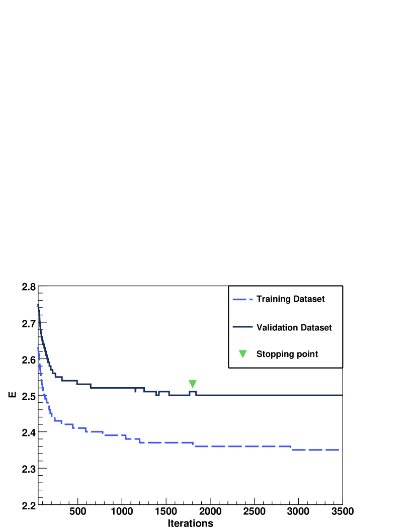
Figure 3: Training and validation error functions as a function of the number of iterations for one of the replicas in the reference fit.

Whereas usually when using a genetic algorithm the figure of merit cannot increase during the minimization, with the weighted training algorithm discussed in Sect. 4.2 the value of the figure of merit during minimization oscillates due to updating of the weights. The wavelength of this oscillation is set by the value of $N_{\rm update}$, i.e. the frequency with which weights are updated. In order to avoid spurious stopping induced by these oscillations, we apply the stopping criterion to moving averages computed over a given number of iterations, namely

$$\langle E_{\mathrm{tr,val}}(i)\rangle\equiv{{1}\over{N_{\mathrm{sm}}}}\sum_{l=i-N_{\mathrm{sm}}+1}^{i}E_{\mathrm{tr,val}}(l)\,.$$ (94)

We take as a default value for the averaging (“smearing”) $N_{\mathrm{sm}}=45$. The value is chosen to be unequal to a multiple of the wavelength and larger than two full periods, in order to minimize spurious fluctuations.

The stopping criteria are then satisfied if the averaged training error function is decreasing

$${{\langle E_{\mathrm{tr}}(i)\rangle}\over{\langle E_{\mathrm{tr}}(i-\Delta_{\mathrm{smear}})\rangle}}<1-\delta_{\rm tr}\,,$$ (95)

while the averaged validation error function increases

$${{\langle E_{\mathrm{val}}(i)\rangle}\over{\langle E_{\mathrm{val}}(i-\Delta_{\mathrm{smear}})\rangle}}>1+\delta_{\rm val}\,.$$ (96)

The parameters $\delta_{\rm tr}$, $\delta_{\rm val}$ set the accuracy to which the increase and decrease is required in order to be significant. Their value has been determined as $\delta_{\rm tr}=\delta_{\rm val}=10^{-4}$ by verifying that with much larger values (more than an order of magnitude) a significant fraction of fits never stops, while with much smaller values a sizable fraction of fits stops due to fluctuations. Results are unchanged upon moderate variations of the values of $\delta_{\rm tr},\>\delta_{\rm val}$.

A graphical example of how the stopping criterion works in practice is given in Fig. 3, where the moving averaged training and validation error functions Eq. (94) are plotted as a function of the number of generation for one particular replica of our reference fit, whose training has been artificially prolonged beyond stopping point. Overlearning is apparent as a rather small though visible effect: beyond the stopping point the training figure of merit keeps decreasing steadily while the validation flattens out and actually rises by a small amount. The smallness of the rise is a consequence of the fact that the data set is very large and mostly quite consistent with itself.

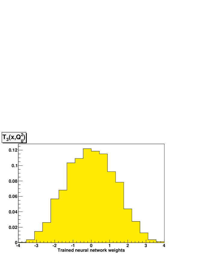
Figure 4: Distribution of neural network weights for $N_{\rm rep}=100$ replicas of the PDF $T_{3}(x,Q^{2})$. The plot shows the percentage of weights which take the value given in abscissa.

In order to avoid unacceptably long fits, when a very large number of iterations $N_{\rm gen}^{\rm max}$ is reached the training is stopped anyway, even if the stopping conditions Eqs. (95,96) are not satisfied. This of course leads to loss of accuracy of the corresponding fits, and it is acceptable provided it only happens for a small fraction of replicas. We will verify that this is indeed the case in Section 5.1. The full set of stopping parameters is summarized in Table 6. We have verified that our final fit is stable against variations of these parameters as well as those of Table 5.

The set of neural nets at stopping provides our best fit, but it is otherwise impossible to endow the best fit values of their parameters with a physical interpretation. In fact, since the nets are redundant, the values of most of these parameters is unconstrained or zero. As an example, the distribution of neural network weights at stopping for 100 replicas of the triplet neural network $T_{3}(x,Q_{0}^{2})$ is displayed in Fig. 4. The well-balanced distribution of weights around zero in Fig. 4 shows that the individual neurons in the neural network operate in their natural range of sensitivity.

5 Results

We have used the methodology discussed in the previous sections to produce a set of parton distributions, which we refer to as the NNPDF1.0 parton set. As discussed in Section 3.6, this parton set is based on five independent parton distributions, corresponding to the two light flavours and the gluon; the strange distribution is assumed to be proportional to the light sea according to Eq. (67), while heavy flavours are generated dynamically using a ZM-VFN scheme, as discussed in Section 3.4. Evolution is performed at NLO as discussed in Sections 3.2-3.3, with $\alpha_{s}(M_{Z}^{2})=0.119$. The heavy quark thresholds are at $m_{c}=Q_{0}=\sqrt{2}$ GeV, $m_{b}=4.3$ GeV and $m_{t}=175$ GeV.

We now present the NNPDF1.0 PDFs, describe some general statistical features of the fits, compare our PDFs to other available parton sets, investigate their statistical uncertainties by discussing their stability with respect to changes in some of the underlying assumptions, and discuss the theoretical uncertainties related to the perturbative order and value of $\alpha_{s}$. We shall then present some results obtained using the NNPDF1.0 set for DIS observables as well as for a few benchmark LHC observables, and compare them to those found using other available sets. The methodology used to obtain estimates for central values and errors from our parton set is summarized and compared to that used with other sets in Appendix B.

5.1 The NNPDF1.0 parton set: statistical features

Our full parton set consists of an ensemble of $N_{\mathrm{rep}}=1000$ sets of five PDFs. The general statistical features of the global fit are summarized in Tables 8-7. Here $\langle{\rm TL}\rangle$ denotes the average number of iterations of the genetic algorithm at stopping, as defined in Sect. 4.2-4.3. The other statistical estimators are defined in Appendix B of Ref. [44]

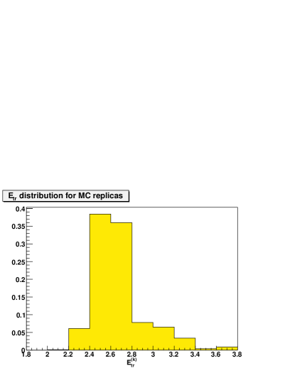
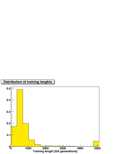
Figure 5: Left: distribution of $E^{(k)}_{\rm tr}$ and of ${\rm TL}^{(k)}$ among the set of trained replicas. The percentage value in given in the $y$ axis.

The distribution of values of the error function Eq. (90) at stopping is displayed in Fig. 5 along with the distribution of training lengths. The former appears to be approximately gaussian and the latter approximately poissonian, with a long tail which causes a slight accumulation of points at $N_{\rm gen}^{\rm max}=5000$ iterations (see Table 6). This may cause a loss in accuracy in outlier fits, which however make up fewer than 5% of the total sample. For completeness, we also show in Fig. 6 the distribution of values of the $\chi^{2}$ of a global fit to the data obtained by using each individual replica PDF set, instead of the best-fit PDF set, whose shape is very similar to that of the distribution of error functions.

The features of the fit can be summarized as follows:

• The $\chi^{2}$ of the central fit (obtained averaging over all PDFs in the sample) is about half of the average value $\langle E\rangle$ of the error function Eq. (90) which measures the quality of the fit of each set to its corresponding replica. This is as expected for a fit which correctly reproduces a “true” behaviour underlying a set of experimental data [42, 43, 44], given that replicas fluctuate about the experimental measurements, which in turn fluctuate about “true” values. It thus supports the use of this central fit as our best fit (see Appendix B). A similar conclusion is obtained by comparing the distribution of values of the error function of Fig. 5 with the distribution of values of the $\chi^{2}$ shown in Fig. 6.

• The quality of the central fit as measured by its $\chi^{2}=1.34$ is close to its expected value. With several thousands of data points, the statistical fluctuations of $\chi^{2}$ are of order of a few percent; moreover, the inaccuracy of the NLO theory used here is likely to contribute 5-10% percent to the value of $\chi^{2}$. Therefore, this value of $\chi^{2}$ might indicate some minor data inconsistency. We shall come back to the issue of the self-consistency of the data in Sect. 5.5.

• The quality of the fit to individual experiments is fairly uniform. The $\chi^{2}$ only grows somewhat larger for the NMC experiment, which is known to have consistency problems [43, 28].

• The uncertainty of the fit, as measured by the standard deviation $\langle\sigma\rangle$ is rather smaller than that of the experimental data: $0.014$ versus $0.055$. Correspondingly, the correlation $\langle\rho\rangle$ between pairs of data points is larger by almost the same factor in the fit than in the experimental data. This can be either a consequence of the fact that the fit is biased by an exceedingly restrictive parametrization, or that it is reproducing an underlying physical law which the data consistently follow [42, 43, 28]. We will show in Sect. 5.4 that the former possibility is strongly disfavoured. Therefore, we conclude that the latter is the case: this reinforces the conclusion that our central fit provides an optimal best fit to the data.

$\chi^{2}_{\mathrm{tot}}$	1.34
$\left\langle E\right\rangle$	2.71
$\left\langle E_{\rm tr}\right\rangle$	2.68
$\left\langle E_{\rm val}\right\rangle$	2.72
$\left\langle{\rm TL}\right\rangle$	824
$\left\langle\sigma^{(\exp)}\right\rangle_{\mathrm{dat}}$	$5.6~{}10^{-2}$
$\left\langle\sigma^{(\mathrm{net})}\right\rangle_{\mathrm{dat}}$	$1.4~{}10^{-2}$
$\left\langle\rho^{(\exp)}\right\rangle_{\mathrm{dat}}$	0.15
$\left\langle\rho^{(\mathrm{net})}\right\rangle_{\mathrm{dat}}$	0.40
$\left\langle{\rm cov}^{(\exp)}\right\rangle_{\mathrm{dat}}$	$1.0~{}10^{-3}$
$\left\langle{\rm cov}^{(\mathrm{net})}\right\rangle_{\mathrm{dat}}$	$1.6~{}10^{-4}$

Table 7: Statistical estimators for the final PDF set with $N_{\mathrm{rep}}=1000$ for the total data set.

Experiment	$\chi^{2}_{\mathrm{tot}}$	$\left\langle E\right\rangle$	$\left\langle\sigma^{(\exp)}\right\rangle_{\mathrm{dat}}$	$\left\langle\sigma^{(\mathrm{net})}\right\rangle_{\mathrm{dat}}$	$\left\langle\rho^{(\exp)}\right\rangle_{\mathrm{dat}}$	$\left\langle\rho^{(\mathrm{net})}\right\rangle_{\mathrm{dat}}$	$\left\langle\rm cov^{(\exp)}\right\rangle_{\mathrm{dat}}$	$\left\langle\rm cov^{(\mathrm{net})}\right\rangle_{\mathrm{dat}}$
SLAC	1.27	3.23	$1.0~{}10^{-2}$	$6.0~{}10^{-3}$	0.31	0.69	$3.1~{}10^{-5}$	$2.6~{}10^{-5}$
BCDMS	1.59	3.10	$7.0~{}10^{-3}$	$3.9~{}10^{-3}$	0.47	0.55	$2.9~{}10^{-5}$	$9.3~{}10^{-6}$
NMC	1.70	3.01	$1.7~{}10^{-2}$	$7.2~{}10^{-3}$	0.16	0.67	$4.4~{}10^{-4}$	$3.4~{}10^{-5}$
NMC-pd	1.53	2.98	$1.5~{}10^{-2}$	$1.2~{}10^{-2}$	$3.3~{}10^{-2}$	0.40	$6.5~{}10^{-6}$	$5.0~{}10^{-5}$
ZEUS	1.11	2.53	$6.1~{}10^{-2}$	$1.0~{}10^{-2}$	$7.9~{}10^{-2}$	0.28	$1.5~{}10^{-4}$	$2.6~{}10^{-5}$
H1	1.03	2.41	$4.7~{}10^{-2}$	$1.0~{}10^{-2}$	$2.7~{}10^{-2}$	0.27	$4.9~{}10^{-2}$	$2.5~{}10^{-5}$
CHORUS	1.40	2.77	0.11	$2.7~{}10^{-2}$	$9.4~{}10^{-2}$	0.43	$2.2~{}10^{-3}$	$3.3~{}10^{-4}$
FLH108	1.62	2.61	0.17	$1.5~{}10^{-2}$	0.65	0.77	$2.0~{}10^{-2}$	$1.8~{}10^{-4}$

Table 8: Statistical estimators for the final PDF set with $N_{\mathrm{rep}}=1000$ for individual experiments.

Figure 6: Distribution of $\chi^{2}$ to the fit to actual data of each replica. The percentage value in given in the $y$ axis.

5.2 The NNPDF1.0 parton set: results

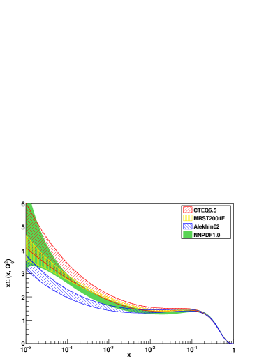
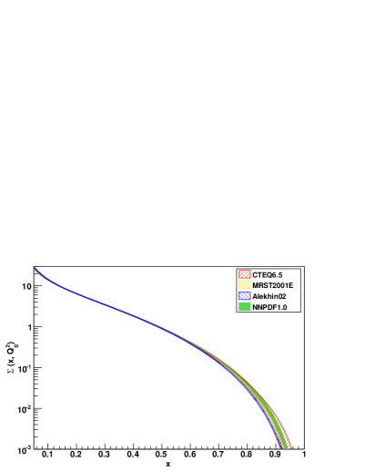
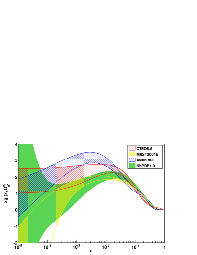
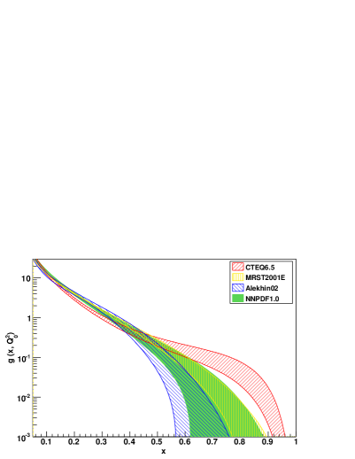
Figure 7: The singlet and gluon PDF at the starting scale $Q_{0}^{2}=2$ GeV², plotted versus $x$ on a log (left) or linear scale (right).

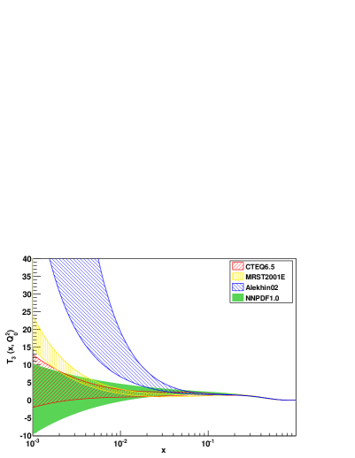
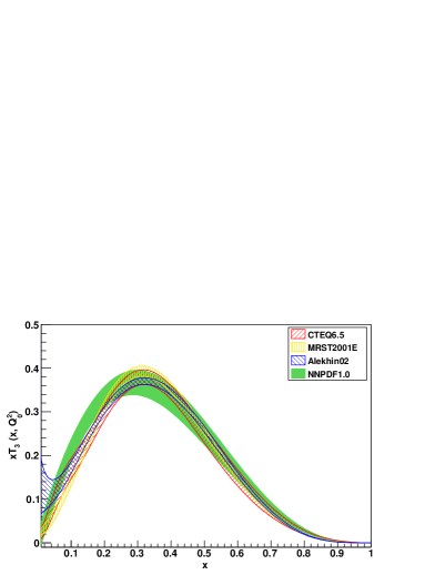
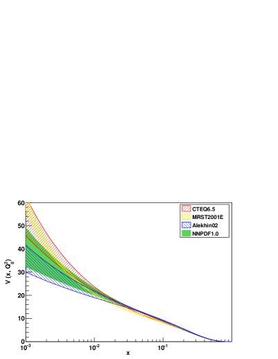
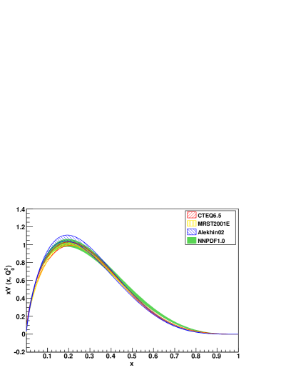
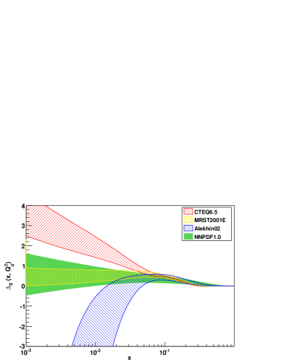
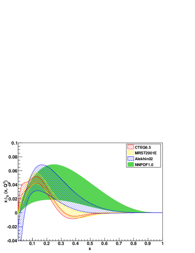
Figure 8: The valence and nonsinglet PDFs at the starting scale $Q_{0}^{2}=2$ GeV², plotted versus $x$ on a log (left) or linear scale (right).

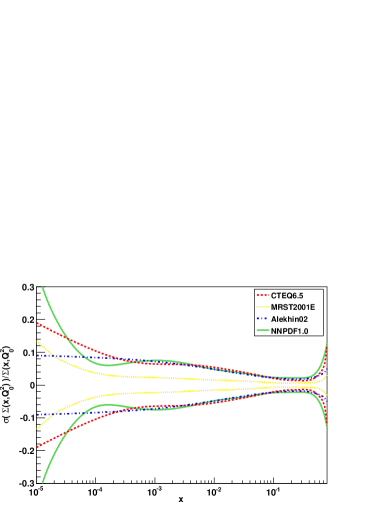
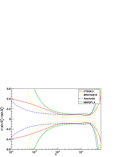
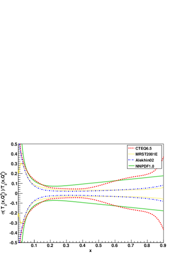
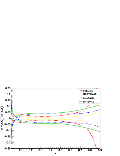
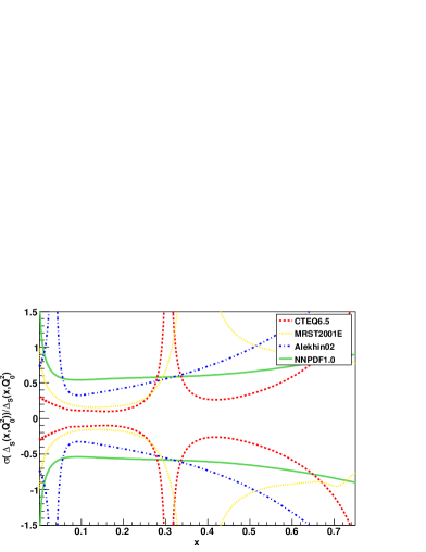
Figure 9: Relative uncertainty on PDFs. All bands correspond to one $\sigma$ (see Appendix B).

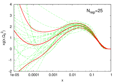
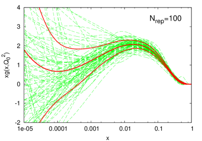
Figure 10: Sets of 25 replicas (left) and 100 replicas (right) of the gluon distribution. The solid red (dark) lines show the average and one-sigma intervals computed from the given sets.

The NNPDF1.0 set of parton distributions at the starting scale $Q_{0}^{2}=2$ GeV² is displayed in Fig. 7 (singlet sector) and Fig. 8 (valence sector), as a function of $x$ both on a linear and a logarithmic scale. The PDFs shown are those which we adopt as a basis set, given in Eq. (87), from which other PDFs can be obtained by linear combination. Relative uncertainties on these PDFs are shown in Fig. 9. Results are compared to those of the other parton sets CTEQ6.5 [30], MRST2001E [33] and Alekhin02 [88], which are the most recent NLO sets from the respective groups available through the LHAPDF interface [89, 90]. All uncertainties in these plots (including those of other parton sets) correspond to nominal one-$\sigma$ error bands. In Fig. 10 we also show the shape of individual replicas and the error band computed for two sets of 25 and 100 replicas of the gluon PDF.

The values of the momentum and valence sum rules computed from NNPDF1.0 using Eqs. (68-69) are correct to within one part per mille, as expected from the accuracy of the numerical integration noted in Sec. 4.1.

The general features of the PDF set can be summarized as follows:

• Even though individual replicas may fluctuate significantly (see Fig. 10) thereby showing the flexibility of the neural parametrization, this appears to be due to statistical fluctuations of the underlying replica data: average quantities, such as the central value and error band shown in the figure, are smooth, all the more so as stability is reached as the number of replicas increases. It is clear from the plot that with $N_{\rm rep}=100$ replicas the results for central values and error bands have stabilized already, as we shall discuss in more detail in Sect. 5.4 below.

• The central values of all PDFs are in reasonable agreement with those from other parton sets, especially in the region where data are available.

• Even though the uncertainty band on the gluon allows for a negative PDF for $x\mathrel{\hbox to0.0pt{\lower 4.0pt\hbox{\hskip 1.0pt$\sim$}\hss}\raise 1.0pt\hbox{$<$}}10^{-4}$, positivity of $F_{L}$ holds for $x\geq 10^{-5}$ and $Q^{2}\geq Q_{0}^{2}$.

• Uncertainties on PDFs in the region where data are available tend to be generally a little larger than those of the CTEQ6.5 and Alekhin02 sets, and rather larger than those of the MRST2001E sets. Note that the one-$\sigma$ uncertainty band that we find without having to introduce a tolerance is thus comparable to or larger than the one-$\sigma$ uncertainty bands obtained by the CTEQ and MRST-MSTW groups with their respective tolerance criteria, which amount to an upward rescaling of all experimental uncertainties by a factor between four and six.

• Uncertainties on PDFs in the region where no data are available tend to be larger than with any other set: this applies to the singlet and gluon at very small $x$, to the valence and triplet at small $x$, and to the gluon at large $x$.

• Some aspects of the NNPDF1.0 PDFs are unconstrained by data which are used in the CTEQ and MRST global fits but not in the data set of Tab. 1. This includes the $\bar{u}-\bar{d}$ asymmetry, which in global fits is mostly constrained by Drell-Yan data, and the large $x$ gluon, which in global fits is constrained by the large-$E_{T}$ jet data. Hence, the wider uncertainty bands found for these quantities are likely to be at least partly due to the smaller data set used in the present fit.

5.3 Parton-parton correlations

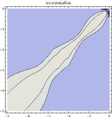
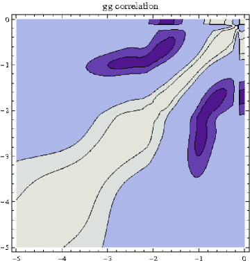
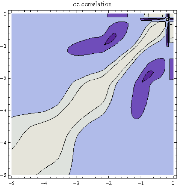
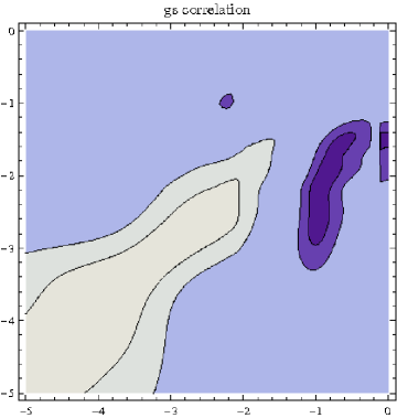
Figure 11: Correlations between PDFs, computed using Eq. (97). The correlations shown are $u-u$ (upper left), $g-g$ (upper right), $c-c$ (lower left) and $g-s$ (lower right, $g$ in abscissa). The labels on the axes are the logarithm to base ten of $x_{1}$ and $x_{2}$. All the correlations are computed at $Q=85$ GeV.

Besides the uncertainty bands on the PDFs, it is interesting to also determine the correlations between different PDFs in a given set: the relevance of these studies for the assessment of the uncertainties on LHC has been recently emphasized in Ref. [91]. The determination of the correlation between any pair of quantities depending on PDFs using NNPDF1.0 is straightforward, as the correlation can be simply calculated using the covariance as its estimator. For example, the correlation between the two PDF values $q(x_{1},Q_{1}^{2})$ and $\widetilde{q}(x_{2},Q_{2}^{2})$ is determined as

$$\rho\left[q(x_{1},Q_{1}^{2})\widetilde{q}(x_{2},Q_{2}^{2})\right]={{\left\langle q(x_{1},Q_{1}^{2})\widetilde{q}(x_{2},Q_{2}^{2})\right\rangle_{\rm rep}-\left\langle q(x_{1},Q_{1}^{2})\right\rangle_{\mathrm{rep}}\left\langle\widetilde{q}(x_{2},Q_{2}^{2})\right\rangle_{\rm rep}}\over{\sigma_{q}(x_{1},Q_{1}^{2})\sigma_{\widetilde{q}}(x_{2},Q_{2}^{2})}},$$ (97)

with all averages performed on the ensemble of replicas. Results for some selected correlations are displayed in Fig. 11. For ease of comparison, we have chosen the same PDFs and scales that were studied in Ref. [91]. The pattern of correlations is similar to that found and discussed in that reference.

5.4 Statistical uncertainties: parametrization independence

As discussed in Section 1.2, an advantage of the NNPDF approach is that various features of the PDF set can be assessed using standard statistical tools. In this Section, we assess the stability of the fit and the reliability of the error estimate provided with it.

The main estimator used in this analysis is the distance $d[q]$. This is defined as the difference in values between two different predictions for some quantity $q$ obtained from two different ensemble of PDFs, measured in units of the sum in quadrature of their uncertainties: thus if two determinations of $q$ have $d=1$ this means that their difference is equal to the sum in quadrature of their respective uncertainties. (see appendix B of Ref. [44] for a more extensive discussion). We compute this distance for each PDF in turn and for the uncertainty on it, at the starting scale $Q_{0}^{2}=2$ GeV². Specifically, we quote values for the distance in various ranges of $x$, by computing it at ten equally spaced points in $x$ in the given range and averaging the results. In order to guarantee accuracy of the results, the computation is repeated a large number of times over different sets of replicas (of order of a hundred). In practice, since we only have a limited total ensemble of PDFs, the repetitions are performed by taking different subsets of the full ensemble.

At first, we check that the results of the fit are stable when using different subsets of 100 replicas out of the full ensemble of 1000 replicas. Results are shown in Table 9 for all PDFs and corresponding uncertainties, in two kinematical $x$ regions which are schematically identified as a region where the PDF is mostly controlled by data, and a region where it is mostly extrapolated. It is clear that the results of the fits are indeed behaving as they ought to. It is important to notice that distances listed in the table refer to an average over 100 replicas, whose standard deviation is by a factor $\sqrt{N_{\rm rep}}$ smaller than the standard deviation of each of the replicas. Hence, the fact that $d\sim 1$ for two sets of 100 PDFs means that the central values of these PDFs differ by a tenth of the sum in quadrature of their standard deviations. It follows that Table 9 also verifies that indeed the fluctuation of results obtained as an average over $N_{\rm rep}$ replicas scales as $1/\sqrt{N_{\rm rep}}$ as it ought to.

	Data	Extrapolation
$\Sigma(x,Q_{0}^{2})$	$5~{}10^{-4}\leq x\leq 0.1$	$10^{-5}\leq x\leq 10^{-4}$
$\left\langle d[q]\right\rangle$	0.99	0.87
$\left\langle d[\sigma]\right\rangle$	0.96	0.95
$g(x,Q_{0}^{2})$	$5~{}10^{-4}\leq x\leq 0.1$	$10^{-5}\leq x\leq 10^{-4}$
$\left\langle d[q]\right\rangle$	0.98	0.82
$\left\langle d[\sigma]\right\rangle$	1.00	0.96
$T_{3}(x,Q_{0}^{2})$	$0.05\leq x\leq 0.75$	$10^{-3}\leq x\leq 10^{-2}$
$\left\langle d[q]\right\rangle$	0.88	0.76
$\left\langle d[\sigma]\right\rangle$	0.94	0.82
$V(x,Q_{0}^{2})$	$0.1\leq x\leq 0.6$	$3~{}10^{-3}\leq x\leq 3~{}10^{-2}$
$\left\langle d[q]\right\rangle$	0.95	0.82
$\left\langle d[\sigma]\right\rangle$	0.94	0.79
$\Delta_{S}(x,Q_{0}^{2})$	$0.1\leq x\leq 0.6$	$3~{}10^{-3}\leq x\leq 3~{}10^{-2}$
$\left\langle d[q]\right\rangle$	0.75	0.81
$\left\langle d[\sigma]\right\rangle$	0.88	0.82

Table 9: Distance between results obtained from two different sets of 100 PDFs out of the full ensemble of 1000 PDFs.

Next, we study the dependence of results on the architecture of PDFs. Specifically, we reduce the architecture from 2-5-3-1 to 2-4-3-1, thereby decreasing the number of parameters of each PDF from 37 to 31. Results are given in Table 10. We find remarkable stability: fluctuations are at most at the two-$\sigma$ level in poorly controlled quantities, such as the value of the light quark sea asymmetry in the extrapolation region, or the uncertainty on the isotriplet combination in the extrapolation region. This shows that results are indeed independent of the number of parameters.

	Data	Extrapolation
$\Sigma(x,Q_{0}^{2})$	$5~{}10^{-4}\leq x\leq 0.1$	$10^{-5}\leq x\leq 10^{-4}$
$\left\langle d[q]\right\rangle$	0.98	1.25
$\left\langle d[\sigma]\right\rangle$	1.14	1.34
$g(x,Q_{0}^{2})$	$5~{}10^{-4}\leq x\leq 0.1$	$10^{-5}\leq x\leq 10^{-4}$
$\left\langle d[q]\right\rangle$	1.52	1.15
$\left\langle d[\sigma]\right\rangle$	1.16	1.07
$T_{3}(x,Q_{0}^{2})$	$0.05\leq x\leq 0.75$	$10^{-3}\leq x\leq 10^{-2}$
$\left\langle d[q]\right\rangle$	1.00	1.11
$\left\langle d[\sigma]\right\rangle$	1.76	2.27
$V(x,Q_{0}^{2})$	$0.1\leq x\leq 0.6$	$3~{}10^{-3}\leq x\leq 3~{}10^{-2}$
$\left\langle d[q]\right\rangle$	1.30	0.90
$\left\langle d[\sigma]\right\rangle$	1.10	0.98
$\Delta_{S}(x,Q_{0}^{2})$	$0.1\leq x\leq 0.6$	$3~{}10^{-3}\leq x\leq 3~{}10^{-2}$
$\left\langle d[q]\right\rangle$	1.04	1.91
$\left\langle d[\sigma]\right\rangle$	1.44	1.80

Table 10: Distance between results obtained from a sets of 100 PDFs with neural network architecture 2-5-3-1 and a sets of 100 PDFs with neural network architecture 2-4-3-1.

A more subtle issue related to the parametrization is the choice of preprocessing functions, introduced in the relation Eq. (87) between PDFs and their neural network parametrizations. These functions, as discussed in Sect. 4.1, are introduced in order to speed up the training but should not affect final results. We have thus checked the stability of result upon variation of the preprocessing exponents away from their default values, listed in Table 4.

Valence sector			Singlet sector
	$\chi^{2}$	$\left\langle\rm TL\right\rangle$		$\chi^{2}$	$\left\langle\rm TL\right\rangle$
$n_{T_{3}}=n_{V}=0.1$	1.38	771	$n_{\Sigma}=n_{g}=0.8$	1.39	1002
$n_{T_{3}}=n_{V}=0.5$	1.34	1629	$n_{\Sigma}=n_{g}=1.6$	1.52	2287
$m_{T_{3}}=m_{V}=2$	1.55	1186	$m_{\Sigma}=m_{g}-1=2$	1.37	647
$m_{T_{3}}=m_{V}=4$	1.28	1311	$m_{\Sigma}=m_{g}-1=4$	1.41	1306

Table 11: Values of the total $\chi^{2}$ and of the average training length $\left\langle\rm TL\right\rangle$ when preprocessing exponents are varied away from their default values Tab. 4. The value of the exponents which are varied is given for each row.

First, in Table. 11 we display the dependence on preprocessing exponents of the values of the total $\chi^{2}$ and of the average training length $\left\langle\rm TL\right\rangle$. The table shows that in some cases the quality of the fit deteriorates and the average length of training increases significantly when the preprocessing exponents are varied. This implies that in these cases a satisfactory fit has not been obtained: indeed, in such cases there is a noticeable increase in the fraction of replicas which reach the maximum training length of $N_{\rm gen}^{\rm max}=5000$ without achieving convergence. Hence, an increase of $N_{\rm gen}^{\rm max}$, or possibly a more efficient or differently tuned minimization algorithm would be required to obtain a satisfactory fit. Thus, in these cases we expect reduced stability of results: this applies to the case of increase of the small $x$ preprocessing exponent $n$ for the singlet, and to a lesser extent to the decrease of the large $x$ preprocessing exponent $m$ for the nonsinglet and valence.

Data region
	$n_{v}=0.1$	$n_{v}=0.5$	$m_{v}=2$	$m_{v}=4$	$n_{s}=0.8$	$n_{s}=1.6$	$m_{s}=2$	$m_{s}=4$
$\Sigma(x,Q_{0}^{2})$
$\left\langle d[q]\right\rangle$	1.34	1.25	1.37	2.14	1.72	1.38	1.45	1.64
$\left\langle d[\sigma]\right\rangle$	1.45	1.44	1.25	1.44	2.03	2.66	0.95	1.35
$g(x,Q_{0}^{2})$
$\left\langle d[q]\right\rangle$	1.31	1.30	2.69	1.15	3.06	2.08	1.20	1.74
$\left\langle d[\sigma]\right\rangle$	1.34	1.60	1.56	1.37	3.21	2.44	0.98	1.72
$T_{3}(x,Q_{0}^{2})$
$\left\langle d[q]\right\rangle$	1.97	2.48	8.35	9.74	1.31	3.23	1.03	1.41
$\left\langle d[\sigma]\right\rangle$	1.10	1.47	1.98	1.53	1.10	2.66	1.76	1.99
$V(x,Q_{0}^{2})$
$\left\langle d[q]\right\rangle$	11.03	1.55	3.61	5.60	0.94	2.12	1.25	3.54
$\left\langle d[\sigma]\right\rangle$	3.57	4.74	4.04	3.09	1.03	1.10	0.66	1.98
$\Delta_{S}(x,Q_{0}^{2})$
$\left\langle d[q]\right\rangle$	2.00	2.29	7.51	2.36	1.14	1.70	0.76	0.92
$\left\langle d[\sigma]\right\rangle$	1.25	5.20	1.17	3.50	1.00	1.98	0.97	2.05

Extrapolation
	$n_{v}=0.1$	$n_{v}=0.5$	$m_{v}=2$	$m_{v}=4$	$n_{s}=0.8$	$n_{s}=1.6$	$m_{s}=2$	$m_{s}=4$
$\Sigma(x,Q_{0}^{2})$
$\left\langle d[q]\right\rangle$	1.06	1.69	1.49	1.84	7.72	4.67	0.87	3.15
$\left\langle d[\sigma]\right\rangle$	1.12	1.84	2.11	1.52	2.47	3.66	0.82	2.34
$g(x,Q_{0}^{2})$
$\left\langle d[q]\right\rangle$	1.41	2.32	2.33	1.34	1.62	4.73	1.04	3.49
$\left\langle d[\sigma]\right\rangle$	1.41	1.86	1.95	1.30	2.15	2.72	0.81	2.38
$T_{3}(x,Q_{0}^{2})$
$\left\langle d[q]\right\rangle$	1.71	2.70	7.40	1.60	1.36	2.37	0.78	0.91
$\left\langle d[\sigma]\right\rangle$	4.83	4.54	2.89	5.09	1.00	1.65	0.92	1.26
$V(x,Q_{0}^{2})$
$\left\langle d[q]\right\rangle$	14.85	3.23	3.75	2.55	0.86	2.52	1.26	1.34
$\left\langle d[\sigma]\right\rangle$	2.65	5.08	3.94	2.78	1.20	0.87	0.62	2.25
$\Delta_{S}(x,Q_{0}^{2})$
$\left\langle d[q]\right\rangle$	1.25	2.50	7.75	2.48	1.09	1.47	1.09	0.83
$\left\langle d[\sigma]\right\rangle$	1.80	2.85	1.50	2.28	0.90	2.01	0.90	1.64

Table 12: Distance between results found with a set of 100 PDFs with the default preprocessing exponents Table 11, and 100 PDFs obtained with a different value of some of the preprocessing exponents. The data and extrapolation regions for each PDF are the same as in Table 9. The preprocessing exponents which are varied are listed in the table, with $n_{v}\equiv n_{T_{3}}=n_{V}$, $m_{v}\equiv m_{T_{3}}=m_{V}$, $n_{s}\equiv n_{\Sigma}=n_{g}$ and $m_{s}\equiv m_{\Sigma}=m_{g}-1$.

In Table 12 we show the distance from the default of results obtained as the preprocessing exponents are varied. In almost all cases, remarkable stability is found, with variation of results well within the 90% confidence level. Even in the case of increase of the singlet $n$ exponent mentioned above reasonable stability is found. A notable exception is the behaviour of the triplet and the valence upon variation of the large or small $x$ exponents. In these cases, the distance is of order ten without significant deterioration of the fit quality: this (with 100 replicas) means that central values differ by about 1.4 $\sigma$ in units of the respective standard deviations. We must conclude that in these cases we do not find complete independence of results on the preprocessing function, and therefore that uncertainties on our quark distributions in the valence region are likely to be underestimated by a factor between one and two. A more faithful estimate of these uncertainties would require for example random variation of the preprocessing exponents within the range where a good fit quality obtains. However, it should be noted that uncertainties on valence PDFs are going to be greatly reduced when Drell-Yan data are included in our data set.

5.5 Statistical uncertainties: dependence on the data set

Set	$N_{\rm dat}$	$x_{\rm min}$	$x_{\rm max}$	$Q^{2}_{\rm min}$	$Q^{2}_{\rm max}$
BCDMSp	322	$7~{}10^{-2}$	0.75	10.3	230
NMC	95	0.028	0.48	9	6
NMC-pd	73	0.035	0.67	11.4	99
Z97NC	206	$1.6~{}10^{-4}$	0.65	10	$2~{}10^{4}$
H197low$Q^{2}$	77	$3.2~{}10^{-4}$	0.2	12	150

Table 13: Reduced data set used for benchmarking.

Having verified the reliability and independence of our results on the parametrization, we perform a series of checks to see how they behave when data are excluded from the fitting set. The aim of these tests is to make sure that our results are not fine-tuned to our choice of a specific data set, and thus that the same approach can lead to satisfactory results with data sets of different sizes and with different features.

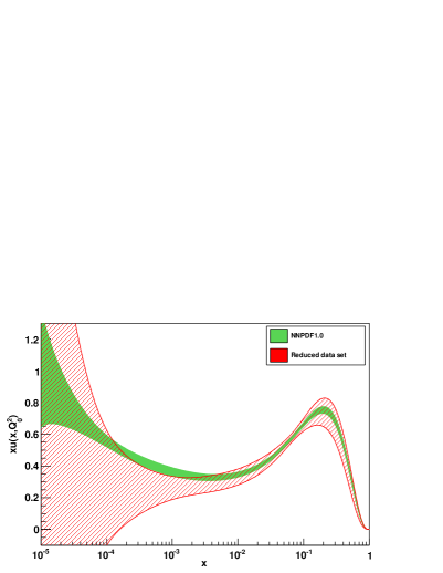
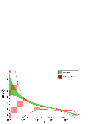
Figure 12: Comparison of the NNPDF1.0 reference PDFs to those obtained from a fit to the reduced data set of Table 13. The PDFs shown at the starting scale $Q_{0}^{2}=2$ GeV² are $u(x)$ (left plot) and $\bar{d}(x)$ (right plot).

At first, we simply reduce our data set to the much smaller set of Table 13, with a total of $N_{\rm dat}=733$ data points, to be compared to the $N_{\rm dat}=3163$ of the full fit. This is the same data set which was used for the benchmark Ref. [41], mentioned in Sect. 1.1. A comparison of the up and antidown PDFs obtained in this way with the ones of the reference fit is shown in Fig. 12. Clearly, as data are removed the uncertainty bands increase in the region where there is information loss (such as large $x$ for the sea and small $x$ for the valence), but central values remain compatible within uncertainties. This shows that the parton parametrization with neural nets is flexible enough to accommodate results from either of these data sets, and it confirms that results are indeed independent of the parametrization.

This increase in error band when data are removed indicates that the data included in the fit are mostly consistent with each other, i.e. they lead to consistent underlying PDF sets. Indeed, if there are systematic data inconsistencies, when the inconsistent data are a small subset of the full data set they will on average be fitted poorly by the best-fit PDFs. This is due to the fact that when these data are included in the training set an improvement of the quality of the fit to them does not generally lead to an improvement of the quality of the fit to the remaining data in the validation set. This behaviour was observed in our fits of Ref. [43], when fitting some NMC structure function data which are known [28] to be somewhat inconsistent with the rest. If instead two sets of data are inconsistent and roughly of the same size, the best fit PDFs will fluctuate between those who give a good fit to either of the datasets, according to which data are randomly included in the training set of each replica. A mild inconsistency of this kind was recently observed in our fits when comparing ZEUS and H1 structure function data [92].

In neither case will the inclusion of inconsistent data lead to a decrease of the uncertainty, and in the latter case it might even lead to an increase of the uncertainty, if the systematic discrepancy between the two datasets is sizably larger than the uncertainty of each of them. In all cases, inconsistencies will be signalled by a large value of the $\chi^{2}$ of the best fit. The behaviour displayed in Fig. 12, together with the low value of the $\chi^{2}=1.34$ in Table 7, suggests that only minor insonsistencies are present in the NNPDF1.0 dataset, although the mild inconsistencies such as those within the NMC dataset and between H1 and ZEUS datasets mentioned above are likely to be present.

A more detailed check of stability can be performed by removing data in a fixed kinematic region. To this purpose, we repeat the reference fit but with the cut in $Q^{2}$ raised from the default $Q_{\rm cut}^{2}$=2 GeV² to $Q_{\rm cut}^{2}$=10 GeV². As can be seen from Fig. 2, this removes from the analysis a sizable amount of data, leaving $N_{\rm dat}=2355$ out of the $N_{\rm dat}=3163$ of the reference fit. Results found in this case are displayed in Fig. 13, which clearly shows the increased uncertainty in the small $x$ region where data have been removed, and good stability in the valence region where the data set is essentially unchanged.

	Data/Data	Data/Extrapolation	Extrapolation/Extrapolation
$\Sigma(x,Q_{0}^{2})$	$3~{}10^{-3}\leq x\leq 0.1$	$5~{}10^{-4}\leq x\leq 10^{-3}$	$5~{}10^{-5}\leq x\leq 10^{-4}$
$\left\langle d[q]\right\rangle$	2.48	8.04	5.79
$\left\langle d[\sigma]\right\rangle$	2.85	3.73	4.43
$g(x,Q_{0}^{2})$	$3~{}10^{-3}\leq x\leq 0.1$	$5~{}10^{-4}\leq x\leq 10^{-3}$	$5~{}10^{-5}\leq x\leq 10^{-4}$
$\left\langle d[q]\right\rangle$	4.27	6.12	5.04
$\left\langle d[\sigma]\right\rangle$	3.06	3.04	2.03
$T_{3}(x,Q_{0}^{2})$	$0.2\leq x\leq 0.75$	$5~{}10^{-1}\leq x\leq 0.1$	$10^{-3}\leq x\leq 10^{-2}$
$\left\langle d[q]\right\rangle$	2.33	2.00	0.53
$\left\langle d[\sigma]\right\rangle$	1.62	1.34	1.14
$V(x,Q_{0}^{2})$	$0.3\leq x\leq 0.6$	$0.1\leq x\leq 0.2$	$3~{}10^{-3}\leq x\leq 3~{}10^{-2}$
$\left\langle d[q]\right\rangle$	0.88	1.42	1.15
$\left\langle d[\sigma]\right\rangle$	1.09	1.89	1.62
$\Delta_{S}(x,Q_{0}^{2})$	$0.3\leq x\leq 0.6$	$0.1\leq x\leq 0.2$	$3~{}10^{-3}\leq x\leq 3~{}10^{-2}$
$\left\langle d[q]\right\rangle$	2.54	2.29	0.92
$\left\langle d[\sigma]\right\rangle$	1.13	1.13	1.15

Table 14: Distance between results computed from a set of $N_{\rm rep}=100$ replicas from the reference fit and a set of $N_{\rm rep}=100$ replicas from a fit where the kinematic cut in $Q^{2}$ has been raised from $Q_{\rm min}^{2}=2$ GeV² to $Q_{\rm min}^{2}=10$ GeV².

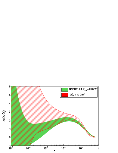
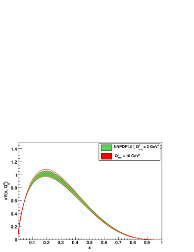
Figure 13: Comparison of the reference fit to a fit in which where the kinematical cut in $Q^{2}$ has been raised from $Q_{\rm min}^{2}=2$ GeV² to $Q_{\rm min}^{2}=10$ GeV². The gluon (left plot) and the total valence PDFs (right plot) are shown.

This is assessed in a quantitative way in Table 14, by tabulating the distance between results in the three kinematic regions (a) where data are available both before and after raising the cut (Data/Data); (b) where there are data before raising the cut but not afterwards (Data/Extrapolation); (c) where there are no data either with the lower or higher cut (Extrapolation/Extrapolation). In most cases we find good stability at the 90% confidence level: as shown in Fig. 13 whenever central values change significantly, the uncertainties increase correspondingly.

An interesting exception is the case of the Data/Extrapolation region for singlet and gluon. This is the kinematic region of most of the HERA data: raising the cut corresponds to excluding the HERA data from the fit. In this case, even though the central reference is within the uncertainty band of the fit with the higher cut (see Fig. 13), the distance between central values is rather larger than allowed by statistical fluctuations. This can be understood as a consequence of the fact that the behaviour of the gluon at small $x$ in the HERA region cannot be predicted by simple extrapolation of the behaviour observed at larger $x$ in the NMC region. Similar behaviour was observed in structure function fits [43], though here the problem is alleviated by the fact that for a wide class of starting quark and gluon distributions the shape of structure functions obtained from NLO QCD evolution is universal [93].

	Data	Extrapolation
$\Sigma(x,Q_{0}^{2})$	$5~{}10^{-4}\leq x\leq 0.1$	$10^{-5}\leq x\leq 10^{-4}$
$\left\langle d[q]\right\rangle$	2.13	1.95
$\left\langle d[\sigma]\right\rangle$	1.17	1.83
$g(x,Q_{0}^{2})$	$5~{}10^{-4}\leq x\leq 0.1$	$10^{-5}\leq x\leq 10^{-4}$
$\left\langle d[q]\right\rangle$	1.76	1.82
$\left\langle d[\sigma]\right\rangle$	1.29	1.87
$T_{3}(x,Q_{0}^{2})$	$0.05\leq x\leq 0.75$	$10^{-3}\leq x\leq 10^{-2}$
$\left\langle d[q]\right\rangle$	1.07	0.93
$\left\langle d[\sigma]\right\rangle$	1.17	1.59
$V(x,Q_{0}^{2})$	$0.1\leq x\leq 0.6$	$3~{}10^{-3}\leq x\leq 3~{}10^{-2}$
$\left\langle d[q]\right\rangle$	1.42	1.62
$\left\langle d[\sigma]\right\rangle$	1.56	1.64
$\Delta_{S}(x,Q_{0}^{2})$	$0.1\leq x\leq 0.6$	$3~{}10^{-3}\leq x\leq 3~{}10^{-2}$
$\left\langle d[q]\right\rangle$	0.99	1.71
$\left\langle d[\sigma]\right\rangle$	1.35	1.73

Table 15: Distance between results computed from a set of $N_{\rm rep}=100$ replicas from the reference fit and a set of $N_{\rm rep}=100$ replicas from a fit where the training fraction has been reduced from its default $f_{\rm tr}=0.5$ to $f_{\rm tr}=0.25$.

As a final test, we reduce the number of data points by randomly removing points from the data set. This is simply done by reducing the fraction $f_{\rm tr}$ of points in the training set from its default value $f_{\rm tr}=0.5$ (see Sect. 4.3) to $f_{\rm tr}=0.25$. As shown in Table 15, results move by at most two-$\sigma$ as a consequence. Furthermore, in this case uncertainties are unchanged: for instance, the value of $\left\langle\sigma^{(\mathrm{net})}\right\rangle_{\mathrm{dat}}$ coincides with that of the reference fit given in Tab. 8. Hence, the fit behaves as one expects when the data set is changed, but with no significant information loss. This indicates that the data set is consistent and quite redundant. Of course, if the training fraction were reduced further eventually one would have information loss, and one would be led back to the situation of smaller sets of experiments or kinematic cuts.

5.6 Theoretical uncertainties

Pert. order	LO		NLO		NLO
$\alpha_{s}(M_{Z}^{2})$	0.130		0.117		0.121
$\chi^{2}$	1.41		1.35		1.33
$\left\langle{\rm TL}\right\rangle$	1153		877		736
$\left\langle\sigma^{(\mathrm{net})}\right\rangle_{\mathrm{dat}}$	$1.4~{}10^{-2}$		$1.4~{}10^{-2}$		$1.4~{}10^{-2}$
$\left\langle\rho^{(\mathrm{net})}\right\rangle_{\mathrm{dat}}$	0.41		0.40		0.43
$\left\langle{\rm cov}^{(\mathrm{net})}\right\rangle_{\mathrm{dat}}$	$1.6~{}10^{-4}$		$1.5~{}10^{-4}$		$2.0~{}10^{-4}$
	Data	Extrapolation	Data	Extra	Data	Extra
$\Sigma(x,Q_{0}^{2})$	$5~{}10^{-4}\leq x\leq 0.1$	$10^{-5}\leq x\leq 10^{-4}$
$\left\langle d[q]\right\rangle$	13.42	3.93	1.72	1.05	0.73	0.81
$\left\langle d[\sigma]\right\rangle$	1.38	0.93	1.05	1.03	1.22	0.95
$g(x,Q_{0}^{2})$	$5~{}10^{-4}\leq x\leq 0.1$	$10^{-5}\leq x\leq 10^{-4}$
$\left\langle d[q]\right\rangle$	18.62	6.42	4.68	2.29	4.12	0.71
$\left\langle d[\sigma]\right\rangle$	1.10	2.10	1.00	0.91	0.88	0.83
$T_{3}(x,Q_{0}^{2})$	$0.05\leq x\leq 0.75$	$10^{-3}\leq x\leq 10^{-2}$
$\left\langle d[q]\right\rangle$	3.72	1.33	0.71	0.71	1.55	0.96
$\left\langle d[\sigma]\right\rangle$	1.22	0.92	0.93	0.75	1.11	0.78
$V(x,Q_{0}^{2})$	$0.1\leq x\leq 0.6$	$3~{}10^{-3}\leq x\leq 3~{}10^{-2}$
$\left\langle d[q]\right\rangle$	3.63	2.92	0.92	0.74	1.89	1.72
$\left\langle d[\sigma]\right\rangle$	1.58	1.17	0.94	0.71	0.67	0.65
$\Delta_{S}(x,Q_{0}^{2})$	$0.1\leq x\leq 0.6$	$3~{}10^{-3}\leq x\leq 3~{}10^{-2}$
$\left\langle d[q]\right\rangle$	1.34	1.94	0.74	0.58	0.86	1.36
$\left\langle d[\sigma]\right\rangle$	0.95	1.06	0.67	0.83	0.78	0.76

Table 16: Statistical estimators for the LO fit and the NLO fits with different values of $\alpha_{s}$ (top) and distance between results computed from a set of $N_{\rm rep}=100$ replicas from these fits and set of $N_{\rm rep}=100$ replicas from the reference fit.

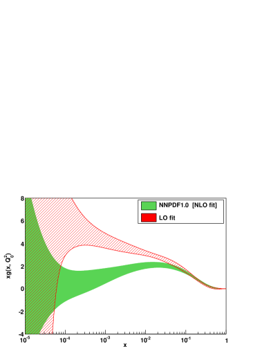
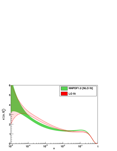
Figure 14: Comparison of the NLO (reference) and LO fit results for the gluon (left) and quark singlet PDFs (right).

In our determination of PDFs, all systematic uncertainties in the data have been accounted for in the Monte Carlo data generation, as discussed in Sect. 2: they are then propagated through the fitting procedure onto our final results. Therefore, error bands on the NNPDF1.0 PDFs already include both statistical and systematic uncertainties on the data. On top of these, however, there exists theoretical uncertainties due to the fact that we do not fit directly experimental observables, but rather PDFs, which are theoretical constructs of QCD, and are thus affected by uncertainties related to incomplete knowledge of the theory: we shall refer to these (sometimes called model uncertainties) as theoretical uncertainties.

The main theoretical uncertainties on NNPDF1.0 are those related to the fact that our analysis is performed at NLO, and thus neglects effects at NNLO and beyond, and to the choice of value of the strong coupling $\alpha_{s}$, which is only known to finite accuracy. To address these issues, we have repeated our fit at LO, and also at NLO with two different values of the strong coupling, $\alpha_{s}(M_{Z}^{2})=0.117$ and $\alpha_{s}(M_{Z}^{2})=0.121$. The results of these studies are summarized in Tab. 16, where we show the statistical features of these fits, to be compared with those of the reference fit Tab. 8, and the distance of the result of these fits from those of the reference.

Comparison of the LO fit to the NLO shows that the quality of the fit deteriorates significantly when using LO theory, as one might expect. However, the size of the uncertainties remains essentially unchanged, as shown by the value of both $\left\langle\sigma^{(\mathrm{net})}\right\rangle_{\mathrm{dat}}$ and of $d[\sigma]$. Furthermore, all central values of the LO fit vary by an amount which is compatible with statistical fluctuations, with the exception of the singlet and gluon, which vary by about two-$\sigma$, as one expects due to the fact that the gluon contribution to deep-inelastic coefficient functions only starts at NLO. The change in behaviour of the singlet and gluon is displayed in Fig. 14.

The comparison of the LO and NLO fits also indicates that the theoretical uncertainty due to lack of inclusion of NNLO corrections is negligible on the scale of statistical uncertainties. This conclusion is based on the observation that NNLO corrections to all PDFs are known [94, 36] to be a fraction of the typical NLO corrections (i.e. the NLO-LO difference) in the nonsinglet sector, which we already find to be smaller by a factor larger than two than statistical uncertainties.

Comparison of the NLO fits with different values of $\alpha_{s}$ shows a variation in $\chi^{2}$ which, though small in terms of the expected statistical fluctuations of the $\chi^{2}$ itself, is actually quite significant in absolute value and thus for the determination of $\alpha_{s}$ (see Ref. [95] for an explanation of this distinction). The possibility of such a determination $\alpha_{s}$ will be explored further in future studies. The change in central values of PDFs is compatible with statistical fluctuations, except in the case of the gluon, as one expects due to the fact that the gluon contribution to deep-inelastic structure functions is of order $\alpha_{s}$. Even in this case, however, the change is a fraction of the statistical uncertainty.

We conclude that the dominant theoretical uncertainties are small on the scale of the statistical uncertainties in our fit. If this will no longer be the case in future analyses, theoretical uncertainties can be taken into account by varying the underlying parameters in a randomized way during the fitting procedure. For example, the uncertainty on the value of $\alpha_{s}$ could be accounted for by taking it as a random variable distributed about its central value with a given uncertainty, and letting it fluctuate between replicas. For the time being, however, this does not appear to be necessary.

Further possible sources of theoretical uncertainty include effects related to large $x$ and small $x$ resummation of the perturbative expansion, the treatment and position of heavy quark thresholds, higher twist corrections, and nuclear effects especially in the treatment of neutrino data. All these corrections are expected to be smaller than those discussed here. They will addressed in future studies as the precision of the analysis improves.

5.7 Usage and delivery of the NNPDF1.0 set

The statistical features of the NNPDF1.0 parton set are those of the full ensemble of $N_{\rm rep}=1000$ replicas. However, as we have explicitly verified in Sect. 5.4, the scaling with the value of $N_{\rm rep}$ of results obtained from NNPDF1.0 works just as one would expect on naive statistical grounds, and therefore a smaller number of replicas may be sufficient for the computation of quantities whose uncertainty decreases fast enough with $N_{\rm rep}$. For example, as is well known [45], the variance of the mean of a sample of size $N_{\mathrm{rep}}$ is $s^{2}/N_{\rm rep}$, where $s$ is the standard deviation of the underlying distribution from which the sample is taken. Similarly, the variance of the variance itself is (for gaussianly distributed quantities) $2s^{4}/(N_{\rm rep}-1)$, Therefore, if the standard deviation corresponds to a 10% uncertainty, a sample of 100 replicas will be sufficient to determine central values with 1% accuracy and the uncertainty itself with 5% accuracy.

The computation of quantities that depend on more detailed statistical features of the sample may be more delicate, and require the use of the full ensemble. An example is the computation of correlations: indeed, not only does the uncertainty on correlations only decrease as $1/\sqrt{N_{\rm rep}}$, but also the correlation computed with the sample is only asymptotically an unbiased estimator, since it overshoots the true one by an amount which only vanishes as $1/N_{\rm rep}$. Therefore, the stability tests of Sects. 5.4-5.5 were computed using sets of $N_{\rm rep}=100$ replicas, but the correlations displayed in Fig. 11 were determined using the full set of $N_{\rm rep}=1000$ replicas.

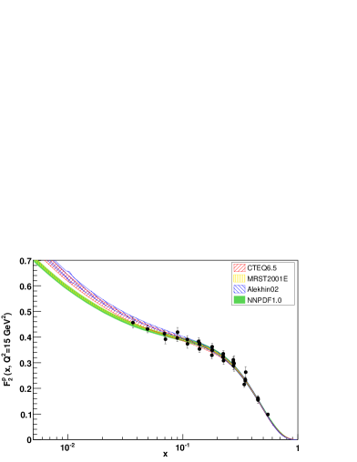
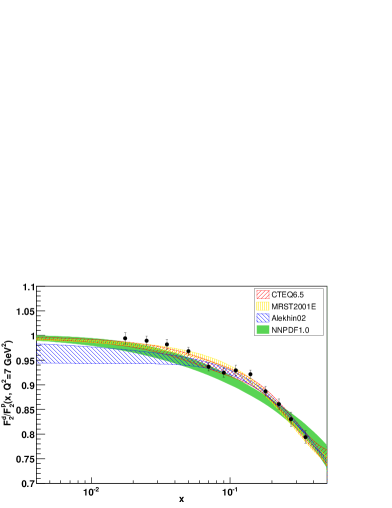
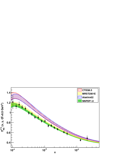
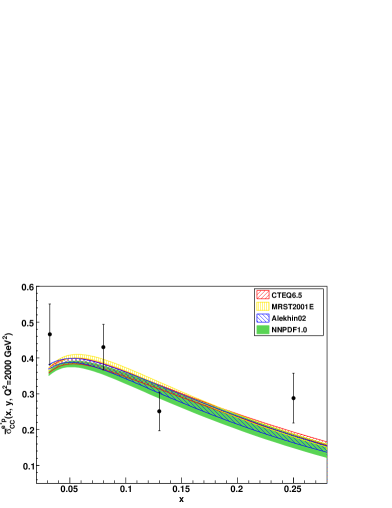
Figure 15: Comparison of NLO theoretical predictions and data for various observables included in the NNPDF fits. First row: proton $F^{p}_{2}$ at $Q^{2}=15$ GeV²(left) and deuteron/proton ratio $F^{d}_{2}/F^{p}_{2}$ at $Q^{2}=7$ GeV² (right). Second row: positron-proton NC (left) and CC (right) reduced cross sections at $Q^{2}=6.5$ GeV². The value of $y$ is determined as a function of $x$ with $\sqrt{s}=301$ GeV. Third row: neutrino-proton total reduced cross-section at $Q^{2}=12$ GeV². The value of $y$ is determined as a function of $x$ with $E_{\nu}=70$ GeV. Theoretical uncertainties are all one-$\sigma$ bands, while experimental error bars are total uncertainties with statistical and systematic errors added in quadrature.

For these reasons, we will provide both the full set 1000 replicas, and a restricted set of 100 replicas. Of course, other sets can be extracted as needed from the full set. The NNPDF1.0 sets can be downloaded from the web site http://sophia.ecm.ub.es/nnpdf/, together with instructions for interfacing to commonly used codes. They can also be accessed through the LHAPDF library [89]. The computation of central values and errors using Monte Carlo PDF sets is briefly summarized in Appendix B.

Given the statistical information contained in the full ensemble of PDFs, it is possible to construct optimized sets which consist of a smaller number of replicas, but whose statistical properties are closer to those of the full ensemble than those of a random subset of it. This can be done by picking, out of the full set, a subset that minimizes a measure of the distance between the probability distribution of the subset and that of the full set, such as the relative entropy (or Kullback–Leibler divergence) [96]. This construction is the subject of current investigation and it will be presented elsewhere.

5.8 Comparison with present and future experimental data

A full study of the phenomenological implications of the NNPDF1.0 parton set is beyond the scope of this work. However, for the sake of illustration, in this section we present first comparisons of theoretical predictions obtained using NNPDF1.0 with data, both for deep-inelastic observables included in the fit and for some LHC observables.

In Fig. 15 the theoretical prediction obtained using NLO QCD and the NNPDF1.0 set is compared to the data, for some representative deep-inelastic observables included in the data set of Table 1. Results obtained using the most recent NLO sets from other groups [30, 33, 88] included in the LHAPDF library [89] are also shown. As one might expect, the differences between predictions obtained using different parton sets are smaller for these observables than they are for the parton distributions themselves (compare Figs. 7-8). This is unsurprising given that these data (with the exception of the CHORUS data) have been used in the determination of all these sets.

In Table 17 and Fig. 16 we show the total cross sections for $W$ and $Z$ production. These processes have been proposed as luminosity monitors at the LHC, but they remain sensitive to various aspects of PDFs [41, 91]. All cross sections have been computed at NLO using MCFM [97, 98, 99, 100], using a sample of $N_{\rm rep}=100$ replicas, which as discussed in Sect. 5.7 is fully adequate for this purpose. The results are compared to those obtained using the MRST2001E [33], CTEQ6.1 [28] and CTEQ6.5 [30] sets. Note that the values given for CTEQ6.5 differ somewhat from those published in Ref. [30], which were however obtained using WTTOT [101]; results for MRST2001E and CTEQ6.1 coincide with those of Ref. [41], also obtained using MCFM.

	$\sigma_{W^{+}}\mathcal{B}_{l^{+}\nu_{l}}$	$\Delta\sigma_{W^{+}}/\sigma_{W^{+}}$	$\sigma_{W^{-}}\mathcal{B}_{l^{-}\nu_{l}}$	$\Delta\sigma_{W^{-}}/\sigma_{W^{-}}$	$\sigma_{Z}\mathcal{B}_{l^{+}l^{-}}$	$\Delta\sigma_{Z}/\sigma_{Z}$
NNPDF1.0	$11.83\pm 0.26$	2.2%	$8.41\pm 0.20$	2.4%	$1.95\pm 0.04$	2.1%
CTEQ6.1	$11.65\pm 0.34$	2.9%	$8.56\pm 0.26$	3.0%	$1.93\pm 0.06$	3.1%
MRST01	$11.71\pm 0.14$	1.2%	$8.70\pm 0.10$	1.1%	$1.97\pm 0.02$	1.0%
CTEQ6.5	$12.54\pm 0.29$	2.3%	$9.19\pm 0.22$	2.4%	$2.07\pm 0.04$	1.9%

Table 17: Cross sections for gauge boson production at the LHC. All quantities have been computed at NLO with MCFM [97, 98, 99, 100] The quoted uncertainty is the one-$\sigma$ band due to the PDF uncertainty only.

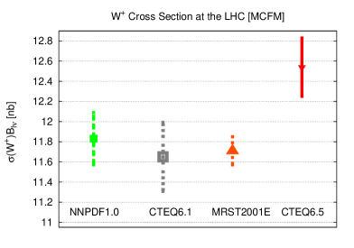
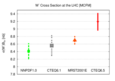
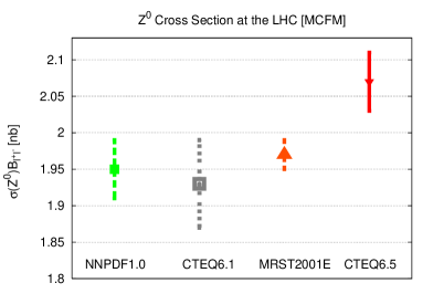
Figure 16: The vector boson production cross sections of Table 17.

We find good agreement of central values with the CTEQ6.1 computation. This is as it should be, given that CTEQ6.1 uses a zero-mass variable-flavour number scheme for heavy quarks as we do (see Sect. 3.4). The difference between results obtained with CTEQ6.1 and CTEQ6.5 is explained in Ref. [91] as a consequence of the different treatment of heavy quark thresholds. The discrepancy between CTEQ6.5 and MRST2001, which use a similar treatment of heavy quark thresholds, is resolved [91] when comparing to the most recent MSTW NNLO set [36]. Our estimate of the uncertainties is a little less than that of the CTEQ fits, but is rather larger than that of MRST. Note however that unlike CTEQ and MRST, NNPDF1.0 does not yet include any Drell-Yan data in the determination of the PDFs.

6 Conclusions and outlook

We have presented a set of parton distributions, determined using a new method which is designed to provide results that are unbiased and amenable to statistical analysis for the probability distribution of PDFs.

The main features of this approach and of the NNPDF1.0 parton set based on it are the following:

• The parton set is given as a Monte Carlo ensemble of replicas of the parton distributions which form the basis of independent PDFs. This ensemble provides a representation of the probability distributions in the space of PDFs, whence any statistical property of the parton distributions themselves or of any function(al) of them can be calculated using standard statistical methods. It is thus easy to compute not only central values and uncertainties, but in fact any desired property such as, for example, the correlation between a certain cross section and, say, the momentum fraction carried by a particular parton distribution.

• The parton parametrization, based on neural networks, is extremely redundant and independence of results on it can be verified explicitly. It is thus possible to verify that the reduction in the uncertainties of the predictions from the fit as compared to those of the input data is due to the combination of many consistent data which obey an underlying physical law, and not to parametrization bias. A small residual dependence of results on the preprocessing in the neural networks can be accurately assessed and monitored.

• A single parton parametrization is flexible enough to reproduce data sets of different sizes, as demonstrated by the fact that as data are removed, uncertainty bands increase to accommodate the increasingly large fluctuations of central values. This in particular implies that uncertainty bands in the region where there are no data are determined by interpolation or extrapolation of the fluctuations observed in the data region, and not by the form of the parametrization.

• Results behave according to standard statistical expectations upon changes in the size of the Monte Carlo ensemble. This enables the consistent use of samples of different size according to the quantity one wishes to compute: for example, a small sample is often sufficient for the accurate determination of an average thanks to the fact that the variance of the average of $N$ quantities is smaller by a factor $1/N$ than the variance of each of them.

• Uncertainty bands are produced directly from the propagation through the Monte Carlo and fitting procedure of the uncertainty on the underlying data, and do not require the use of any tolerance criterion.

• The best fit is not determined as the absolute minimum for a given functional form, but rather it is found by the cross-validation method of comparing to the quality of the fit to a (randomly selected) control data sample. As a consequence, inconsistent data or underestimated uncertainties do not require a separate treatment, and are automatically accounted for and signalled by a larger than average value of the $\chi^{2}$ per degree of freedom.

The results discussed here provide a first full parton set based on this novel methodology, which can be improved in many respects. The main improvements which we envisage are the following:

• A wider set of data besides deep-inelastic scattering should be included. This will improve the accuracy of quantities such as the gluon at large $x$ (from jet data) or the light antiquark sea asymmetry (from Drell-Yan data), and it will make possible a direct determination of the strange distribution which we did not determine here.

• Heavy quark thresholds should be treated more accurately, by including terms proportional to the heavy quark mass, i.e. to ${{m^{2}_{H}}\over{Q^{2}}}$. Because heavy quark distributions are generated radiatively by matching in the threshold region, this improves the accuracy in the determination of heavy quark fractions at high scale.

• Complete independence of the preprocessing of neural networks should be obtained by randomizing the preprocessing functions, as discussed in Sect. 5.4. Similarly contributions from theoretical uncertainties such as the choice of factorization scale could be included by randomizing the corresponding parameters, as discussed in Sect. 5.6.

• A set of LO parton distributions should be produced in view of its use in Monte Carlo generators (see Ref. [102]). A set of NNLO parton distributions should be produced, both with the purpose of estimating uncertainties on the NLO results and also for some precision applications. Sets of partons including large and small $x$ resummation corrections should also be considered.

• An optimized small set of parton distributions should be produced which reproduces as closely as possible the statistical features of the full set, as briefly discussed in Sect. 5.7. This would then allow the efficient computation of detailed statistical features without having to use the full ensemble of a thousand replicas.

None of these improvements (with the possible exception of the last) requires conceptually new tools: they can all be made by straightforward generalizations of the techniques discussed here. Many of them will become relevant only as the quality and accuracy of the fit improves. More importantly, it will be possible to monitor this improvement, since we now have at our disposal a statistically reliable and accurate PDF fitting tool.

Acknowledgements
This work was partly supported by grants ANR-05-JCJC-0046-01 (France), PRIN-2006 (Italy), MEC FIS2004-05639-C02-01 (Spain) and by the European network HEPTOOLS under contract MRTN-CT-2006-035505. L.D.D. is funded by an STFC Advanced Fellowship and M.U. by a SUPA graduate studentship. We thank S. Alekhin, M. Arneodo, B. Cousins, G. d’Agostini, A. de Roeck, J. Feltesse, W. Giele, A. Glazov, S. Keller, D. Mason, P. Nadolsky, E. Perez, M. Pierini, K. Rabberts, G. Salam, D. Soper, M. Spiropulu, R. Thorne, W. K. Tung for discussions and correspondence. We thank M. Cacciari for help in cross-checking the implementation of NNPDF, and M. Whalley for help with the LHAPDF interface. We are especially grateful to the following people for helping us to understand the features of various data sets: J. Ferrando, C. Gwenlan and E. Tassi for ZEUS, V. Radescu, E. Rizvi and F. Zomer for H1, R. Oldeman for CHORUS and V. Lenderman for the H1 $F_{L}$ data.

Appendix A Kernels for Physical Observables

In this appendix we expand the physical observables — structure functions for DIS from protons and deuterons (measured by SLAC, BCDMS and NMC), the reduced cross-sections for neutral and charged current DIS from protons (measured by ZEUS and H1), and the neutrino cross-sections from a deuteron target (measured by CHORUS) — in the basis of PDFs given in Sec. 3.4, Eqs. (55-3.4). This yields explicit expressions for the Mellin transforms of the hard kernels, in the form Eq. (70), which after Mellin inversion Eq. (71) can then be used to compute the observables through evaluation of the convolutions (72,73) with the initial PDFs determined from the neural nets Eq. (87).

The expressions below can be used with evolution kernels and coefficients evaluated at any order in perturbation theory. Currently evolution kernels $\Gamma_{\rm NS}^{\pm,v}$ and $\Gamma_{\rm S}^{ij}$, $i,j=q,g$, described in Sec. 3.2, can be computed at NLO [69, 70, 71, 72, 73, 74] and NNLO [75, 76], while the DIS coefficient functions $C_{I,i}$, $I=2,3,L$, $i=q,g$ are known at NLO [103], NNLO [104, 105, 106, 107, 108] and NNNLO [109, 110, 111, 112]. Note that at NLO $\Gamma_{\rm NS}^{v}=\Gamma_{\rm NS}^{-}=\Gamma_{\rm NS}^{24}=\Gamma_{\rm NS}^{35}$, $C^{s}_{I,q}=C_{I,q}$, while at LO $\Gamma_{\rm NS}^{+}=\Gamma_{\rm NS}^{-}=\Gamma_{\rm NS}^{v}=\Gamma_{\rm S}^{qq}$ and $C_{I,g}=C_{L,q}=0$, while $C_{2,q}=C_{3,q}=1$.

The heavy quark evolution factors $\Gamma_{\rm S}^{24,i}$, $\Gamma_{\rm S}^{35,i}$, $i=q,g$ in the ZM-VFNS are given in Eqs. (62,64). Below the top threshold we can set $\Gamma_{\rm S}^{35,q}=\Gamma_{\rm S}^{qq}$, $\Gamma_{\rm S}^{35,g}=\Gamma_{\rm S}^{qg}$, while below the $b$ threshold $\Gamma_{\rm S}^{24,q}=\Gamma_{\rm S}^{35,q}=\Gamma_{\rm S}^{qq}$, $\Gamma_{\rm S}^{24,g}=\Gamma_{\rm S}^{35,g}=\Gamma_{\rm S}^{qg}$, with some simplification of the results.

Throughout this section we use a condensed notation in which the arguments of $f_{i}$, $F_{I}$, $\Gamma$, $C$ and $K$ are all suppressed: parton distributions evaluated at $Q_{0}^{2}$ are denoted by a subscript $0$, e.g. $\Sigma_{0}\equiv\Sigma(x,Q_{0}^{2})$. We will assume throughout that $Q_{0}^{2}=m_{c}^{2}$, as explained in Sec. 3.4.We also assume that $b=\bar{b}$, i.e. $V_{24}=V$ at $Q^{2}=m_{b}^{2}$, and similarly $t=\bar{t}$, i.e. $V_{35}=V$ at $Q^{2}=m_{t}^{2}$. However we do allow for the possibility of intrinsic charm, even though for the parton fits described in this paper this option is not exercised. The specific flavour assumptions described in Sec. 3.6 can be summarised as $T_{8,0}=\hbox{${{2-2C_{s}}\over{2+C_{s}}}$}\Sigma_{0}+\hbox{${{3C_{s}}\over{2+C_{s}}}$}V_{0}$, (see Eq. (67)), $T_{15,0}=\Sigma_{0}$, $V_{8,0}=V_{15,0}=V_{0}$.

Target mass corrections are included in the kernels using the procedure described in Sec. 3.8.

A.1 Structure Functions: SLAC, BCDMS and NMC

The datasets we include in our analysis include measurements of $F_{2}^{p}$, $F_{2}^{d}$ and the ratio $F_{2}^{d}/F_{2}^{p}$. These observables can be written in terms of the linear combinations of parton densities used in the evolution code (defined in Eq. (55) and Eq. (3.4)): in the quark model the proton structure function

$$F_{2}^{p}=x\sum_{i=1}^{n_{f}}e_{i}^{2}q_{i}^{+}=x\{\hbox{${{5}\over{18}}$}\Sigma+\hbox{${{1}\over{6}}$}T_{3}+\hbox{${{1}\over{18}}$}(T_{8}-T_{15})+\hbox{${{1}\over{30}}$}(T_{24}-T_{35})\},$$ (98)

where $e_{i}$ are the quark charges (${{2}\over{3}}$ for $u,c,t$, $-\hbox{${{1}\over{3}}$}$ for $d,s,b$), while the deuteron structure function

$$F_{2}^{d}=\hbox{${{1}\over{2}}$}(F_{2}^{p}+F_{2}^{n})=x\{\hbox{${{5}\over{18}}$}\Sigma+\hbox{${{1}\over{18}}$}(T_{8}-T_{15})+\hbox{${{1}\over{30}}$}(T_{24}-T_{35})\}\,.$$ (99)

In perturbative QCD, we have

$$F_{2}^{p} = x\{\hbox{${{5}\over{18}}$}C^{s}_{2,q}\otimes\Sigma+\hbox{${{1}\over{6}}$}C_{2,q}\otimes(T_{3}+\hbox{${{1}\over{3}}$}(T_{8}-T_{15})+\hbox{${{1}\over{5}}$}(T_{24}-T_{35}))$$ (100)

$$\qquad\qquad\qquad\qquad\qquad\qquad+{\langle e_{q}^{2}\rangle}C_{2,g}\otimes g\},$$

$$F_{2}^{d} = x\{\hbox{${{5}\over{18}}$}C^{s}_{2,q}\otimes\Sigma+\hbox{${{1}\over{6}}$}C_{2,q}\otimes(\hbox{${{1}\over{3}}$}(T_{8}-T_{15})+\hbox{${{1}\over{5}}$}(T_{24}-T_{35}))+{\langle e_{q}^{2}\rangle}C_{2,g}\otimes g\}\,.$$ (101)

where $\otimes$ denotes the Mellin convolution, defined in Eq. (19), and ${\langle e_{q}^{2}\rangle}$ is defined as

$${\langle e_{q}^{2}\rangle}=\hbox{${{1}\over{n_{f}}}$}\sum_{i=1}^{n_{f}}e_{i}^{2},$$ (102)

where $n_{f}$ is the number of active flavours: ${\langle e_{q}^{2}\rangle}=\hbox{${{2}\over{9}}$},\hbox{${{5}\over{18}}$},\hbox{${{11}\over{45}}$},\hbox{${{5}\over{18}}$}$ for $n_{f}=3,4,5,6$. We can thus write

$$F_{2}^{p} = x\{K_{{\rm F2},\Sigma}\otimes\Sigma_{0}+K_{{\rm F2},g}\otimes g_{0}+K_{{\rm F2},+}\otimes\left(T_{3,0}+\hbox{${{1}\over{3}}$}(T_{8,0}-T_{15,0})\right)\},$$ (103)

$$F_{2}^{d} = x\{K_{{\rm F2},\Sigma}\otimes\Sigma_{0}+K_{{\rm F2},g}\otimes g_{0}+\hbox{${{1}\over{3}}$}K_{{\rm F2},+}\otimes\left(T_{8,0}-T_{15,0}\right)\},$$ (104)

where (in Mellin space)

$$K_{{\rm F2},\Sigma} = \hbox{${{5}\over{18}}$}C^{s}_{2,q}\Gamma_{\rm S}^{qq}+\hbox{${{1}\over{30}}$}C_{2,q}(\Gamma_{\rm S}^{24,q}-\Gamma_{\rm S}^{35,q})+{\langle e_{q}^{2}\rangle}C_{2,g}\Gamma_{\rm S}^{gq},$$ (105)

$$K_{{\rm F2},g} = \hbox{${{5}\over{18}}$}C^{s}_{2,q}\Gamma_{\rm S}^{qg}+\hbox{${{1}\over{30}}$}C_{2,q}(\Gamma_{\rm S}^{24,g}-\Gamma_{\rm S}^{35,g})+{\langle e_{q}^{2}\rangle}C_{2,g}\Gamma_{\rm S}^{gg},$$ (106)

$$K_{{\rm F2},+} = \hbox{${{1}\over{6}}$}C_{2,q}\Gamma_{\rm NS}^{+}.$$ (107)

A.2 Neutral Current Reduced Cross-Sections: ZEUS and H1

For high energy DIS experiments, as is the case for ZEUS and H1, the contribution from weak boson exchange cannot be neglected.

The neutral current deep-inelastic scattering reduced cross section Eq. (9) is

$$\widetilde{\sigma}^{\rm NC,e^{\pm}}=F_{2}^{NC}\mp\hbox{${{Y_{-}}\over{Y_{+}}}$}xF_{3}^{NC}-\hbox{${{y^{2}}\over{Y_{+}}}$}F_{L}^{NC},$$ (108)

with $Y_{\pm}=1\pm(1-y)^{2}$. In the quark model

$$F_{2}^{\rm NC}=F_{2}^{\gamma}+\sum_{i=1}^{n_{f}}\,B_{i}\,q^{+}_{i},\qquad F_{3}^{\rm NC}=\sum_{i=1}^{n_{f}}\,D_{i}\,q_{i}^{-},$$ (109)

where $F_{2}^{\gamma}$ is the purely electromagnetic structure function, and the charge factors are

$$B_{q}(Q^{2}) = -2e_{q}V_{e}V_{q}P_{Z}+(V_{e}^{2}+A_{e}^{2})(V_{q}^{2}+A_{q}^{2})P_{Z}^{2},$$ (110)

$$D_{q}(Q^{2}) = -2e_{q}A_{e}A_{q}P_{Z}+4V_{e}A_{e}V_{q}A_{q}P_{Z}^{2},$$ (111)

fermions	$e_{f}$	$V_{f}$	$A_{f}$
u,c,t	+2/3	$(+1/2-4/3\sin^{2}\theta_{W})$	+1/2
d,s,b	-1/3	$(-1/2+2/3\sin^{2}\theta_{W})$	-1/2
$\nu_{e},\nu_{\mu},\nu_{\tau}$	0	+1/2	+1/2
e,$\mu,\tau$	-1	$(-1/2+2\sin^{2}\theta_{W})$	-1/2

Table 18: Coupling of fermions to the Z boson.

where $P_{Z}\equiv Q^{2}/(Q^{2}+M_{Z}^{2})$, $V_{f}$ and $A_{f}$ are the vector and axial couplings of the fermions to the Z boson, as given in Table 18. In terms of the PDF evolution eigenstates Eq. (55-3.4)

$$F_{2}^{\rm NC} = x\{E_{\rm S}^{+}\Sigma+E_{\rm NS}^{+}(T_{3}+\hbox{${{1}\over{3}}$}(T_{8}-T_{15})+\hbox{${{1}\over{5}}$}(T_{24}-T_{35}))\},$$ (112)

$$F_{3}^{\rm NC} = E_{\rm S}^{-}V+E_{\rm NS}^{-}(V_{3}+\hbox{${{1}\over{3}}$}(V_{8}-V_{15})+\hbox{${{1}\over{5}}$}(V_{24}-V_{35})),$$ (113)

where the charge coefficients

$$E_{\rm S}^{+} = \hbox{${{5}\over{18}}$}+\hbox{${{1}\over{2}}$}(B_{u}+B_{d}),\qquad E_{\rm NS}^{+}=\hbox{${{1}\over{6}}$}+\hbox{${{1}\over{2}}$}(B_{u}-B_{d}),$$

$$E_{\rm S}^{-} = \hbox{${{1}\over{2}}$}(D_{u}+D_{d}),\qquad E_{\rm NS}^{-}=\hbox{${{1}\over{2}}$}(D_{u}-D_{d}),$$ (114)

In perturbative QCD we can thus write the reduced cross sections as

$$\widetilde{\sigma}^{\rm NC,e^{\pm}}=x\{(C^{s}_{2,q}-\hbox{${{y^{2}}\over{Y_{+}}}$}C^{s}_{L,q})\otimes E_{\rm S}^{+}\Sigma+E_{g}(C_{2,g}-\hbox{${{y^{2}}\over{Y_{+}}}$}C_{L,g})\otimes g$$

$$\qquad+(C_{2,q}-\hbox{${{y^{2}}\over{Y_{+}}}$}C_{L,q})\otimes(E_{\rm NS}^{+}(T_{3}+\hbox{${{1}\over{3}}$}(T_{8}-T_{15})+\hbox{${{1}\over{5}}$}(T_{24}-T_{35})))$$

$$\qquad\mp\hbox{${{Y_{-}}\over{Y_{+}}}$}C_{3,q}\otimes(E_{\rm S}^{-}V+E_{\rm NS}^{-}(V_{3}+\hbox{${{1}\over{3}}$}(V_{8}-V_{15}))),\}$$ (115)

where we have set $V_{24}=V_{35}=V$, and

$$E_{g}={\langle e_{q}^{2}\rangle}+{\langle B_{q}^{2}\rangle},$$ (116)

where

$${\langle B_{q}^{2}\rangle}=\hbox{${{1}\over{n_{f}}}$}\sum_{i=1}^{n_{f}}B_{i}=\begin{cases}\hbox{${{1}\over{3}}$}\left(B_{u}+2B_{d}\right),&{\rm if}\quad n_{f}=3,\\ \hbox{${{1}\over{2}}$}\left(B_{u}+B_{d}\right),&{\rm if}\quad n_{f}=4,\\ \hbox{${{1}\over{5}}$}\left(2B_{u}+3B_{d}\right),&{\rm if}\quad n_{f}=5,\\ \hbox{${{1}\over{2}}$}\left(B_{u}+B_{d}\right),&{\rm if}\quad n_{f}=6.\end{cases}$$ (117)

Note that the gluon coefficient function $C_{2,g}$ is the same quantity which appears in Eq. (100). In terms of hard kernels, we thus have

$$\widetilde{\sigma}^{\rm NC,e^{\pm}} = x\{K_{{\rm NC},\Sigma}\otimes\Sigma_{0}+K_{{\rm NC},g}\otimes g_{0}+K_{{\rm NC},+}\otimes(T_{3,0}+\hbox{${{1}\over{3}}$}(T_{8,0}-T_{15,0}))$$ (118)

$$\qquad\mp K_{{\rm NC},V}\otimes V_{0}\mp K_{{\rm NC},-}\otimes(V_{3,0}+\hbox{${{1}\over{3}}$}(V_{8,0}-V_{15,0}))\},$$

where in Mellin space

$$K_{{\rm NC},\Sigma} = (C^{s}_{2,q}-\hbox{${{y^{2}}\over{Y_{+}}}$}C^{s}_{L,q})E_{\rm S}^{+}\Gamma_{\rm S}^{qq}+E_{g}(C_{2,g}-\hbox{${{y^{2}}\over{Y_{+}}}$}C_{L,g})\Gamma_{\rm S}^{gq}$$ (119)

$$\qquad\qquad+\hbox{${{1}\over{5}}$}(C_{2,q}-\hbox{${{y^{2}}\over{Y_{+}}}$}C_{L,q})E_{\rm NS}^{+}(\Gamma_{\rm S}^{24,q}-\Gamma_{\rm S}^{35,q}),$$

$$K_{{\rm NC},g} = (C^{s}_{2,q}-\hbox{${{y^{2}}\over{Y_{+}}}$}C^{s}_{L,q})E_{\rm S}^{+}\Gamma_{\rm S}^{qg}+E_{g}(C_{2,g}-\hbox{${{y^{2}}\over{Y_{+}}}$}C_{L,g})\Gamma_{\rm S}^{gg}$$ (120)

$$\qquad\qquad+\hbox{${{1}\over{5}}$}(C_{2,q}-\hbox{${{y^{2}}\over{Y_{+}}}$}C_{L,q})E_{\rm NS}^{+}(\Gamma_{\rm S}^{24,g}-\Gamma_{\rm S}^{35,g}),$$

$$K_{{\rm NC},+} = E_{\rm NS}^{+}(C_{2,q}-\hbox{${{y^{2}}\over{Y_{+}}}$}C_{L,q})\Gamma_{\rm NS}^{+},$$ (121)

$$K_{{\rm NC},V} = E_{\rm S}^{-}\hbox{${{Y_{-}}\over{Y_{+}}}$}C_{3,q}\Gamma_{\rm NS}^{v},\qquad K_{{\rm NC},-}=E_{\rm NS}^{-}\hbox{${{Y_{-}}\over{Y_{+}}}$}C_{3,q}\Gamma_{\rm NS}^{-}.$$ (122)

It is also convenient to write down here the expression for $F_{L}^{\rm NC}$ which we use to fix the positivity constraint and fit the H1 $F_{L}$ data:

$$F_{L}^{\rm NC}=x\{K_{{\rm FL},\Sigma}\otimes\Sigma_{0}+K_{{\rm FL},g}\otimes g_{0}+K_{{\rm FL},+}\otimes\left(T_{3,0}+\hbox{${{1}\over{3}}$}(T_{8,0}-T_{15,0})\right)\},$$ (123)

where

$$K_{{\rm FL},\Sigma} = C^{s}_{L,q}E_{\rm S}^{+}\Gamma_{\rm S}^{qq}+\hbox{${{1}\over{5}}$}C_{L,q}E_{\rm NS}^{+}(\Gamma_{\rm S}^{24,q}-\Gamma_{\rm S}^{35,q})+E_{g}C_{L,g}\Gamma_{\rm S}^{gq},$$ (124)

$$K_{{\rm FL},g} = C^{s}_{L,q}E_{\rm S}^{+}\Gamma_{\rm S}^{qg}+\hbox{${{1}\over{5}}$}C_{L,q}E_{\rm S}^{-}(\Gamma_{\rm S}^{24,g}-\Gamma_{\rm S}^{35,g})+E_{g}C_{L,g}\Gamma_{\rm S}^{gg},$$ (125)

$$K_{{\rm FL},+} = E_{\rm NS}^{+}C_{L,q}\Gamma_{\rm NS}^{+}.$$ (126)

A.3 Charged-current scattering: ZEUS and H1

For charged current deep-inelastic scattering, the reduced cross-section Eq. (11)

$$\widetilde{\sigma}^{{\rm CC},e^{\pm}}=\hbox{${{1}\over{2}}$}(Y_{+}F_{2}^{CC,e^{\pm}}\mp Y_{-}xF_{3}^{CC,e^{\pm}}-y^{2}F_{L}^{CC,e^{\pm}})\ ,$$ (127)

where the factor of a half comes from the average over the helicity of the incoming leptons.

For charged current and neutrino scattering the inclusion of the third generation is more subtle than for neutral current scattering, since the scattering of $W^{\pm}$ involves a transition between $b$ and $t$. In the ZM-VFNS this means that below the top threshold neither $b$ nor $t$ can contribute to the cross-section, even above $b$ threshold [113]. We must thus consider the linear decomposition of the structure functions below and above the top threshold as two separate cases. Of course, all the current data are effectively below top threshold, so the second possibility is at present rather academic.

Below top threshold (but above charm threshold) in the quark model

$$F_{2}^{CC,e^{+}} = 2x\{\bar{u}+d+s+\bar{c}\},\qquad F_{2}^{CC,e^{-}}=2x\{u+\bar{d}+\bar{s}+c\}.$$ (128)

$$F_{3}^{CC,e^{+}} = 2\{-\bar{u}+d+s-\bar{c}\},\qquad\quad F_{3}^{CC,e^{-}}=2\{u-\bar{d}-\bar{s}+c\}.$$ (129)

Below charm threshold both the charm and the strange contributions would be absent. In terms of the PDF evolution eigenstates Eq. (55-3.4) we thus have

$$F_{2}^{CC,e^{\pm}} = x\{(\hbox{${{4}\over{5}}$}\Sigma+\hbox{${{1}\over{5}}$}T_{24})\mp(V_{3}+\hbox{${{1}\over{3}}$}(V_{8}-V_{15})\},$$ (130)

$$F_{3}^{CC,e^{\pm}} = (\hbox{${{4}\over{5}}$}V+\hbox{${{1}\over{5}}$}V_{24})\mp(T_{3}+\hbox{${{1}\over{3}}$}(T_{8}-T_{15}).$$ (131)

The first term in Eq. (130) is subtle: $(\hbox{${{4}\over{5}}$}\Sigma+\hbox{${{1}\over{5}}$}T_{24})=u^{+}+d^{+}+s^{+}+c^{+}$ both above and below the $b$ threshold, so the $b$ quarks do not couple to the $W^{\pm}$, consistent with Eq. (128). Similar considerations apply to the first term in Eq. (131). In perturbative QCD we thus have

$$F_{2}^{CC,e^{\pm}} = x\{C^{s}_{2,q}\otimes(\hbox{${{4}\over{5}}$}\Sigma+\hbox{${{1}\over{5}}$}T_{24})\mp C_{2,q}\otimes(V_{3}+\hbox{${{1}\over{3}}$}(V_{8}-V_{15}))$$ (132)

$$\qquad\qquad\qquad\qquad\qquad\qquad+r_{f}C_{2,g}\otimes g\},$$

$$F_{L}^{CC,e^{\pm}} = x\{C^{s}_{L,q}\otimes(\hbox{${{4}\over{5}}$}\Sigma+\hbox{${{1}\over{5}}$}T_{24})\mp C_{L,q}\otimes(V_{3}+\hbox{${{1}\over{3}}$}(V_{8}-V_{15}))$$ (133)

$$\qquad\qquad\qquad\qquad\qquad\qquad+r_{f}C_{L,g}\otimes g\},$$

$$F_{3}^{CC,e^{\pm}} = C^{s}_{3,q}\otimes(\hbox{${{4}\over{5}}$}V+\hbox{${{1}\over{5}}$}V_{24})\mp C_{3,q}\otimes\left(T_{3}+\hbox{${{1}\over{3}}$}(T_{8}-T_{15})\right),$$ (134)

where the factor $r_{f}$ counts the proportion of active flavors: denoting with $[n]$ the integer part of $n$,

$$r_{f}=[n_{f}/2]/(n_{f}/2)=\begin{cases}1~{}~{}~{}~{}~{}~{}~{}\hbox{when}~{}n_{f}~{}\hbox{is even}\\ 1-{{1}\over{n_{f}}}~{}\hbox{when}~{}n_{f}~{}\hbox{ is odd.}\end{cases}$$ (135)

The gluon coefficient functions are the same quantities which appear in Eqs. (100,A.2). We can thus write the reduced cross sections as

$$\widetilde{\sigma}^{\rm CC,e^{\pm}} = \hbox{${{1}\over{2}}$}x\{K_{{\rm CC},\Sigma}\otimes\Sigma_{0}+K_{{\rm CC},g}\otimes g_{0}+K_{{\rm CC},+}\otimes(T_{3,0}+\hbox{${{1}\over{3}}$}(T_{8,0}-T_{15,0}))$$ (136)

$$\qquad\mp K_{{\rm CC},V}\otimes V_{0}\mp K_{{\rm CC},-}\otimes(V_{3,0}+\hbox{${{1}\over{3}}$}(V_{8,0}-V_{15,0}))\},$$

where in Mellin space

$$K_{{\rm CC},\Sigma} = \left(Y_{+}C^{s}_{2,q}-y^{2}C^{s}_{L,q}\right)(\hbox{${{4}\over{5}}$}\Gamma_{\rm S}^{qq}+\hbox{${{1}\over{5}}$}\Gamma_{\rm S}^{24,q})$$ (137)

$$\qquad\qquad\qquad+r_{f}\left(Y_{+}C_{2,g}-y^{2}C_{L,g}\right)\Gamma_{\rm S}^{gq},$$

$$K_{{\rm CC},g} = \left(Y_{+}C^{s}_{2,q}-y^{2}C^{s}_{L,q}\right)(\hbox{${{4}\over{5}}$}\Gamma_{\rm S}^{qg}+\hbox{${{1}\over{5}}$}\Gamma_{\rm S}^{24,g})$$ (138)

$$\qquad\qquad\qquad+r_{f}\left(Y_{+}C_{2,g}-y^{2}C_{L,g}\right)\Gamma_{\rm S}^{gg},$$

$$K_{{\rm CC},+} = Y_{-}C_{3,q}\Gamma_{\rm NS}^{+},$$ (139)

$$K_{{\rm CC},V} = Y_{-}C^{s}_{3,q}(\hbox{${{4}\over{5}}$}\Gamma_{\rm NS}^{v}+\hbox{${{1}\over{5}}$}\Gamma_{\rm NS}^{24}),$$ (140)

$$K_{{\rm CC},-} = \left(Y_{+}C_{2,q}-y^{2}C_{L,q}\right)\Gamma_{\rm NS}^{-}.$$ (141)

Above top threshold, $K_{{\rm CC},\Sigma}$, $K_{{\rm CC},g}$ and $K_{{\rm CC},V}$ become instead

$$K^{t}_{{\rm CC},\Sigma} = \left(Y_{+}C^{s}_{2,q}-y^{2}C^{s}_{L,q}\right)\Gamma_{\rm S}^{qq}+r_{f}\left(Y_{+}C_{2,g}-y^{2}C_{L,g}\right)\Gamma_{\rm S}^{gq}$$ (142)

$$\qquad\qquad\qquad+\hbox{${{1}\over{5}}$}Y_{-}C_{3,q}(\Gamma_{\rm S}^{24,q}-\Gamma_{\rm S}^{35,q}),$$

$$K^{t}_{{\rm CC},g} = \left(Y_{+}C^{s}_{2,q}-y^{2}C^{s}_{L,q}\right)\Gamma_{\rm S}^{qg}+r_{f}\left(Y_{+}C_{2,g}-y^{2}C_{L,g}\right)\Gamma_{\rm S}^{gg}$$ (143)

$$\qquad\qquad\qquad+\hbox{${{1}\over{5}}$}Y_{-}C_{3,q}(\Gamma_{\rm S}^{24,g}-\Gamma_{\rm S}^{35,g}),$$

$$K^{t}_{{\rm CC},V} = Y_{-}C^{s}_{3,q}\Gamma_{\rm NS}^{v}+\hbox{${{1}\over{5}}$}\left(Y_{+}C_{2,q}-y^{2}C_{L,q}\right)(\Gamma_{\rm NS}^{24}-\Gamma_{\rm NS}^{35}).$$ (144)

A.4 Neutrino Scattering: CHORUS

The cross-section for high energy neutrino scattering off an isoscalar nucleon is given by Eq. (2.3), which we write as

$$\widetilde{\sigma}^{\nu(\bar{\nu})}=\kappa[\widetilde{Y}_{+}F_{2}^{\nu(\bar{\nu})}-y^{2}F_{L}^{\nu(\bar{\nu})}\pm\,Y_{-}\,xF_{3}^{\nu(\bar{\nu})}],$$ (145)

where $\kappa=G_{F}^{2}M_{N}/(2\pi(1+Q^{2}/M_{W}^{2})^{2})$, $\widetilde{Y}_{+}=Y_{+}-2M^{2}_{N}x^{2}y^{2}/Q^{2}$.

Remembering that the target is isoscalar, in the quark model below the top threshold, but above charm threshold,

$$F_{2}^{\nu} = x\{u+\bar{u}+d+\bar{d}+2s+2\bar{c}\},\qquad F_{2}^{\bar{\nu}}=x\{u+\bar{u}+d+\bar{d}+2\bar{s}+2c\},$$ (146)

$$F_{3}^{\nu} = u-\bar{u}+d-\bar{d}+2s-2\bar{c},\qquad F_{3}^{\bar{\nu}}=u-\bar{u}+d-\bar{d}-2\bar{s}+2c.$$ (147)

Below charm threshold both the charm and the strange contributions would be absent. Of course these expressions can be easily deduced from Eqs. (128,129), since

$$F^{\nu,p}_{2,L,3}=F^{CC,e^{+}}_{2,L,3},\qquad F^{\bar{\nu},p}_{2,L,3}=F^{CC,e^{-}}_{2,L,3}.$$ (148)

In terms of the PDF evolution eigenstates Eq. (55-3.4) we now have in perturbative QCD

$$F_{2}^{\nu(\bar{\nu})} = x\{C^{s}_{2,q}\otimes(\hbox{${{4}\over{5}}$}\Sigma+\hbox{${{1}\over{5}}$}T_{24})\mp\hbox{${{1}\over{3}}$}C_{2,q}\otimes(V_{8}-V_{15})+r_{f}C_{2,g}\otimes g\},$$ (149)

$$F_{L}^{\nu(\bar{\nu})} = x\{C^{s}_{L,q}\otimes(\hbox{${{4}\over{5}}$}\Sigma+\hbox{${{1}\over{5}}$}T_{24})\mp\hbox{${{1}\over{3}}$}C_{L,q}\otimes(V_{8}-V_{15})+r_{f}C_{L,g}\otimes g\},$$ (150)

$$F_{3}^{\nu(\bar{\nu})} = \,C^{s}_{3,q}\otimes(\hbox{${{4}\over{5}}$}V+\hbox{${{1}\over{5}}$}V_{24})\mp\hbox{${{1}\over{3}}$}C_{3,q}\otimes(T_{8}-T_{15}),$$ (151)

the $b$ threshold being accommodated in the same way as in Eq. (132), and with $r_{f}$ defined as in Eq. (135) We can thus write the neutrino cross sections as

$$\widetilde{\sigma}^{\nu(\bar{\nu})} = \kappa\,x\{K_{\nu,\Sigma}\otimes\Sigma_{0}+K_{\nu,g}\otimes g_{0}+K_{\nu,+}\otimes\hbox{${{1}\over{3}}$}(T_{8,0}-T_{15,0})$$ (152)

$$\qquad\mp K_{\nu,V}\otimes V_{0}\mp K_{\nu,-}\otimes\hbox{${{1}\over{3}}$}(V_{8,0}-V_{15,0})\},$$

where in Mellin space

$$K_{\nu,\Sigma} = \left(\widetilde{Y}_{+}C^{s}_{2,q}-y^{2}C^{s}_{L,q}\right)(\hbox{${{4}\over{5}}$}\Gamma_{\rm S}^{qq}+\hbox{${{1}\over{5}}$}\Gamma_{\rm S}^{24,q})$$ (153)

$$\qquad\qquad\qquad+r_{f}\left(\widetilde{Y}_{+}C_{2,g}-y^{2}C_{L,g}\right)\Gamma_{\rm S}^{gq},$$

$$K_{\nu,g} = \left(\widetilde{Y}_{+}C^{s}_{2,q}-y^{2}C^{s}_{L,q}\right)(\hbox{${{4}\over{5}}$}\Gamma_{\rm S}^{qg}+\hbox{${{1}\over{5}}$}\Gamma_{\rm S}^{24,g})$$ (154)

$$\qquad\qquad\qquad+r_{f}\left(\widetilde{Y}_{+}C_{2,g}-y^{2}C_{L,g}\right)\Gamma_{\rm S}^{gg},$$

$$K_{\nu,+} = Y_{-}C_{3,q}\Gamma_{\rm NS}^{+},$$ (155)

$$K_{\nu,V} = Y_{-}C^{s}_{3,q}(\hbox{${{4}\over{5}}$}\Gamma_{\rm NS}^{v}+\hbox{${{1}\over{5}}$}\Gamma_{\rm NS}^{24}),$$ (156)

$$K_{\nu,-} = (\widetilde{Y}_{+}C_{2,q}-y^{2}C_{L,q})\Gamma_{\rm NS}^{-}.$$ (157)

Appendix B Computation of PDF uncertainties

Within our approach, the expectation value of any function $\mathcal{F}[\{q\}]$ which depends on the PDFs is computed as an average over the ensemble of PDFs, using the master formula

$$\left\langle\mathcal{F}[\{q\}]\right\rangle={{1}\over{N_{\rm set}}}\sum_{k=1}^{N_{\rm set}}\mathcal{F}[\{q^{(k)}\}],$$ (158)

where $N_{\rm set}=N_{\rm rep}$ is the number of sets of PDFs in the ensemble, equal to the number of replicas. The associated uncertainty is found as the standard deviation of the sample, according to the usual formula

$$\sigma_{\mathcal{F}} = \left({{N_{\rm set}}\over{N_{\rm set}-1}}\left(\left\langle\mathcal{F}[\{q\}]^{2}\right\rangle-\left\langle\mathcal{F}[\{q\}]\right\rangle^{2}\right)\right)^{1/2}$$ (159)

$$= \left({{1}\over{N_{\rm set}-1}}\sum_{k=1}^{N_{\rm set}}\left(\mathcal{F}[\{q^{(k)}\}]-\left\langle\mathcal{F}[\{q\}]\right\rangle\right)^{2}\right)^{1/2}.$$

These formulae may also be used for the determination of central values and uncertainties of the parton distribution themselves, in which case the functional $\mathcal{F}$ is identified with the parton distribution $q$ : $\mathcal{F}[\{q\}]\equiv q$.

A full discussion of statistical estimators for our PDF set, including correlators and covariances, is given in Appendix B of Ref. [44]. Here we briefly compare the procedures we use to determine central values and errors with those used for the various other PDFs available through HEPDATA.

Available methods for the determination of PDF uncertainties fall broadly into two distinct categories, which we shall refer to as the HEPDATA method (used as a default in the PDF server at the HEPDATA database [19]) and the Monte Carlo method. In both methods sets of PDFs with uncertainties are given as an ensemble of $N_{\rm set}$ sets of PDFs,

$$\{q^{(k)}\}\ ,\qquad k=0,\ldots,N_{\rm set}.$$ (160)

Conventionally the PDF set $q^{(0)}$ corresponds to a “central” set.

In the HEPDATA method, the central set is a best fit set of PDFs, which thus provides the central value for PDFs themselves. The central value of any quantity $\mathcal{F}[\{q\}]$ is obtained in this method by evaluating it as a function of the central set:

$$\mathcal{F}^{(0)}=\mathcal{F}[\{q^{(0)}\}].$$ (161)

In the Monte Carlo method, the central values of any quantity $\mathcal{F}[\{q\}]$ is instead given by Eq. (158). Therefore, the central value for PDFs themselves is given by

$$q^{(0)}\equiv\left\langle q\right\rangle={{1}\over{N_{\rm set}}}\sum_{k=1}^{N_{\rm set}}q^{(k)}\ .$$ (162)

This set is provided as set $q^{(0)}$ in the NNPDF1.0 PDFs. Hence, in the Monte Carlo method the central (best fit) PDF is obtained as an average of the replica best fits. However, for any quantity $\mathcal{F}[\{q\}]$ which depends nonlinearly on the PDFs

$$\left\langle\mathcal{F}[\{q\}]\right\rangle\not=\mathcal{F}[\{q^{(0)}\}].$$ (163)

Hence, Eq. (158) must be used for the determination of the central value, and use of the set $q^{(0)}$ is not recommended. However, for a quantity that does depend linearly on the PDFs, such as a DIS structure function, Eq. (161) with the central PDFs Eq. (162) gives the same result as Eq. (158), and thus it may be used also with the Monte Carlo method. Note that set $q^{(0)}$ should not be included when computing an average with Eq. (158), because it is itself already an average.

The determination of uncertainties with the HEPDATA method is based on the idea that sets $q^{(k)}$ with $k>0$ provide upper and lower variations (for even and odd values of $k$) away from the central set $q^{(0)}$ which correspond to eigenvectors in parameter space. The one-$\sigma$ uncertainty is then found by adding in quadrature these variations:

$$\sigma_{\mathcal{F}}^{\rm hepdata}={{1}\over{2C_{90}}}\left(\sum_{k=1}^{N_{\rm set}/2}\left(\mathcal{F}[\{q^{(2k-1)}\}]-\mathcal{F}[\{q^{(2k)}\}]\right)^{2}\right)^{1/2},$$ (164)

where the factor

$$C_{90}\equiv\sqrt{2}{\rm Erf}^{-1}[0.90]=1.64485$$ (165)

accounts for the fact that the upper and lower parton sets correspond to 90% confidence levels rather than to one-$\sigma$ uncertainties. This method should be used with the CTEQ and MRST/MSTW sets Refs. [28, 29, 30, 31, 32, 33, 34, 35, 36].

A slightly different application of the HEPDATA method is required for the Alekhin PDF sets Ref. [38, 94, 39, 40]. With these PDFs, sets $q^{(k)}$ with $k>0$ each provide the uncertainty limits from the central set, with upper and lower PDFs symmetrical by construction and already corresponding to one-$\sigma$ uncertainties. So for these PDFs

$$\sigma_{\mathcal{F}}^{\rm hepdata}=\left(\sum_{k=1}^{N_{\rm set}}\left(\mathcal{F}[\{q^{(k)}\}]-\mathcal{F}[\{q^{(0)}\}]\right)^{2}\right)^{1/2}.$$ (166)

In the Monte Carlo method, instead, the one-$\sigma$ uncertainty is found using the variance formula Eq. (159). This formula should be used not only for the NNPDF1.0 sets, but also for the parton sets of Refs. [27, 25, 37].

References

- [1] R. McElhaney and S.F. Tuan, Phys. Rev. D8 (1973) 2267.
- [2] T. Kawaguchi and H. Nakkagawa, Analysis of Scaling Violation in Terms of Theories with Anomalous Dimensions, KUNS 380, 1976.
- [3] A. De Rujula, H. Georgi and H.D. Politzer, Ann. Phys. 103 (1977) 315.
- [4] P.W. Johnson and W.k. Tung, Nucl. Phys. B121 (1977) 270.
- [5] M. Gluck and E. Reya, Phys. Rev. D14 (1976) 3034.
- [6] I. Hinchliffe and C.H. Llewellyn Smith, Nucl. Phys. B128 (1977) 93.
- [7] A.J. Buras and K.J.F. Gaemers, Nucl. Phys. B132 (1978) 249.
- [8] NuTeV, G.P. Zeller et al., Phys. Rev. Lett. 88 (2002) 091802, hep-ex/0110059.
- [9] M. Gluck, E. Hoffmann and E. Reya, Zeit. Phys. C13 (1982) 119.
- [10] D.W. Duke and J.F. Owens, Phys. Rev. D30 (1984) 49.
- [11] E. Eichten et al., Rev. Mod. Phys. 56 (1984) 579.
- [12] A. Devoto et al., Phys. Rev. D27 (1983) 508.
- [13] R.G. Roberts, The Structure of the proton: Deep inelastic scattering (Cambridge University Press, 1990).
- [14] R.K. Ellis, W.J. Stirling and B.R. Webber, QCD and collider physics (Cambridge University Press, 1996).
- [15] A.D. Martin, R.G. Roberts and W.J. Stirling, Phys. Rev. D37 (1988) 1161.
- [16] M. Diemoz et al., Z. Phys. C39 (1988) 21.
- [17] M. Gluck, E. Reya and A. Vogt, Z. Phys. C48 (1990) 471.
- [18] J.G. Morfin and W.K. Tung, Z. Phys. C52 (1991) 13.
- [19] HEPDATA, http://durpdg.dur.ac.uk/hepdata/pdf.html.
- [20] M. Klein and R. Yoshida, (2008), 0805.3334.
- [21] CTEQ, H.L. Lai et al., Eur. Phys. J. C12 (2000) 375, hep-ph/9903282.
- [22] A.D. Martin et al., Eur. Phys. J. C23 (2002) 73, hep-ph/0110215.
- [23] S. Alekhin, Eur. Phys. J. C10 (1999) 395, hep-ph/9611213.
- [24] V. Barone, C. Pascaud and F. Zomer, Eur. Phys. J. C12 (2000) 243, hep-ph/9907512.
- [25] M. Botje, Eur. Phys. J. C14 (2000) 285, hep-ph/9912439.
- [26] W.T. Giele and S. Keller, Phys. Rev. D58 (1998) 094023, hep-ph/9803393.
- [27] W.T. Giele, S.A. Keller and D.A. Kosower, (2001), hep-ph/0104052.
- [28] J. Pumplin et al., JHEP 07 (2002) 012, hep-ph/0201195.
- [29] J. Huston et al., JHEP 06 (2005) 080, hep-ph/0502080.
- [30] W.K. Tung et al., JHEP 02 (2007) 053, hep-ph/0611254.
- [31] J.F. Owens et al., Phys. Rev. D75 (2007) 054030, hep-ph/0702159.
- [32] H.L. Lai et al., JHEP 04 (2007) 089, hep-ph/0702268.
- [33] A.D. Martin et al., Eur. Phys. J. C28 (2003) 455, hep-ph/0211080.
- [34] A.D. Martin et al., Eur. Phys. J. C35 (2004) 325, hep-ph/0308087.
- [35] A.D. Martin et al., Phys. Lett. B604 (2004) 61, hep-ph/0410230.
- [36] A.D. Martin et al., Phys. Lett. B652 (2007) 292, 0706.0459.
- [37] S.I. Alekhin, Phys. Rev. D63 (2001) 094022, hep-ph/0011002.
- [38] S. Alekhin, Phys. Rev. D68 (2003) 014002, hep-ph/0211096.
- [39] S. Alekhin, JETP Lett. 82 (2005) 628, hep-ph/0508248.
- [40] S. Alekhin, K. Melnikov and F. Petriello, Phys. Rev. D74 (2006) 054033, hep-ph/0606237.
- [41] M. Dittmar et al., (2005), hep-ph/0511119.
- [42] S. Forte et al., JHEP 05 (2002) 062, hep-ph/0204232.
- [43] NNPDF, L. Del Debbio et al., JHEP 03 (2005) 080, hep-ph/0501067.
- [44] NNPDF, L. Del Debbio et al., JHEP 03 (2007) 039, hep-ph/0701127.
- [45] G. Cowan, Statistical data analysis (Oxford University Press, 2002).
- [46] C.M. Bishop, Neural Networks for Pattern Recognition (Oxford University Press, 1995).
- [47] BCDMS, A.C. Benvenuti et al., Phys. Lett. B223 (1989) 485.
- [48] BCDMS, A.C. Benvenuti et al., Phys. Lett. B237 (1990) 592.
- [49] New Muon Collaboration, M. Arneodo et al., Nucl. Phys. B487 (1997) 3, hep-ex/9611022.
- [50] New Muon Collaboration, M. Arneodo et al., Nucl. Phys. B483 (1997) 3, hep-ph/9610231.
- [51] L.W. Whitlow et al., Phys. Lett. B282 (1992) 475.
- [52] H1, C. Adloff et al., Eur. Phys. J. C21 (2001) 33, hep-ex/0012053.
- [53] H1, C. Adloff et al., Eur. Phys. J. C13 (2000) 609, hep-ex/9908059.
- [54] H1, C. Adloff et al., Eur. Phys. J. C19 (2001) 269, hep-ex/0012052.
- [55] H1, C. Adloff et al., Eur. Phys. J. C30 (2003) 1, hep-ex/0304003.
- [56] ZEUS, S. Chekanov et al., Eur. Phys. J. C21 (2001) 443, hep-ex/0105090.
- [57] ZEUS, J. Breitweg et al., Eur. Phys. J. C12 (2000) 411, hep-ex/9907010.
- [58] ZEUS, S. Chekanov et al., Eur. Phys. J. C28 (2003) 175, hep-ex/0208040.
- [59] ZEUS, S. Chekanov et al., Phys. Lett. B539 (2002) 197, hep-ex/0205091.
- [60] ZEUS, S. Chekanov et al., Phys. Rev. D70 (2004) 052001, hep-ex/0401003.
- [61] ZEUS, S. Chekanov et al., Eur. Phys. J. C32 (2003) 1, hep-ex/0307043.
- [62] H1, F.D. Aaron et al., Phys. Lett. B665 (2008) 139, 0805.2809.
- [63] CHORUS, G. Onengut et al., Phys. Lett. B632 (2006) 65.
- [64] ZEUS, S. Chekanov et al., Eur. Phys. J. C42 (2005) 1, hep-ph/0503274.
- [65] CHORUS, http://choruswww.cern.ch/Publications/DIS-data/.
- [66] G. D’Agostini, Bayesian reasoning in data analysis: A critical introduction (World Scientific, 2003).
- [67] A. Vogt, Comput. Phys. Commun. 170 (2005) 65, hep-ph/0408244.
- [68] J. Blumlein, H. Bottcher and A. Guffanti, Nucl. Phys. B774 (2007) 182, hep-ph/0607200.
- [69] E. Floratos, D. Ross and C. Sachrajda, Nucl.Phys. B129 (1977) 66.
- [70] E. Floratos, D. Ross and C. Sachrajda, Nucl.Phys. B152 (1979) 493.
- [71] A. Gonzalez-Arroyo, C. Lopez and F. Yndurain, Nucl.Phys. B153 (1979) 161.
- [72] A. Gonzalez-Arroyo and C. Lopez, Nucl.Phys. B166 (1980) 429.
- [73] E. Floratos, C. Kounnas and R. Lacaze, Nucl.Phys. B192 (1981) 417.
- [74] G. Curci, W. Furmanski and R. Petronzio, Nucl.Phys. B175 (1980) 27.
- [75] S. Moch, J. Vermaseren and A. Vogt, Nucl.Phys. B688 (2004) 101.
- [76] S. Moch, J. Vermaseren and A. Vogt, Phys. Lett. B691 (2004) 129.
- [77] M. Botje, QCDNUM manual, http://www.nikhef.nl/h24/qcdnum/.
- [78] G.P. Salam and J. Rojo, (2008), 0804.3755.
- [79] J. Abate and P. Valko, International Journal for Numerical Methods in Engineering 60 (2003) 979.
- [80] W. Giele et al., (2002), hep-ph/0204316.
- [81] R.S. Thorne, (2007), 0711.2986.
- [82] CHORUS, A. Kayis-Topaksu et al., Nucl. Phys. B798 (2008) 1, 0804.1869.
- [83] NuTeV, M. Goncharov et al., Phys. Rev. D64 (2001) 112006, hep-ex/0102049.
- [84] J. Pumplin, H.L. Lai and W.K. Tung, Phys. Rev. D75 (2007) 054029, hep-ph/0701220.
- [85] G. Altarelli, S. Forte and G. Ridolfi, Nucl. Phys. B534 (1998) 277, hep-ph/9806345.
- [86] G. Altarelli, R.D. Ball and S. Forte, Nucl. Phys. B799 (2008) 199, 0802.0032.
- [87] H. Georgi and H.D. Politzer, Phys. Rev. D14 (1976) 1829.
- [88] S. Alekhin, Phys. Rev. D68 (2003) 014002, hep-ph/0211096.
- [89] LHAPDF, http://projects.hepforge.org/lhapdf/.
- [90] D. Bourilkov, R.C. Group and M.R. Whalley, (2006), hep-ph/0605240.
- [91] P.M. Nadolsky et al., (2008), 0802.0007.
- [92] NNPDF, R.D. Ball et al., Contribution to the proceedings of the 2008 HERA-LHC workshop (in preparation).
- [93] R.D. Ball and S. Forte, Phys. Lett. B335 (1994) 77, hep-ph/9405320.
- [94] S. Alekhin, (2003), hep-ph/0311184.
- [95] J.C. Collins and J. Pumplin, (2001), hep-ph/0105207.
- [96] T.M. Cover and J.A. Thomas, Elements of information theory (Wiley, New York, 1991).
- [97] J.M. Campbell and R.K. Ellis, Phys. Rev. D62 (2000) 114012, hep-ph/0006304.
- [98] J. Campbell and R.K. Ellis, Phys. Rev. D65 (2002) 113007, hep-ph/0202176.
- [99] J. Campbell, R.K. Ellis and F. Tramontano, Phys. Rev. D70 (2004) 094012, hep-ph/0408158.
- [100] MCFM, http://mcfm.fnal.gov/.
- [101] C.P. Yuan, WTTOT (unpublished).
- [102] A. Sherstnev and R.S. Thorne, Eur. Phys. J. C55 (2008) 553, 0711.2473.
- [103] W. Bardeen et al., Phys. Rev. D18 (1978) 3998.
- [104] W. van Neerven and E. Zijlstra, Phys. Lett. B272 (1991) 127.
- [105] W. van Neerven and E. Zijlstra, Phys. Lett. B273 (1991) 476.
- [106] W. van Neerven and E. Zijlstra, Nucl. Phys. B383 (1992) 525.
- [107] W. van Neerven and E. Zijlstra, Phys. Lett. B297 (1992) 377.
- [108] S. Moch and J. Vermaseren, Nucl. Phys. B573 (2000) 853.
- [109] S. Moch, J.A.M. Vermaseren and A. Vogt, Phys. Lett. B606 (2005) 123, hep-ph/0411112.
- [110] J.A.M. Vermaseren, A. Vogt and S. Moch, Nucl. Phys. B724 (2005) 3, hep-ph/0504242.
- [111] S. Moch and M. Rogal, Nucl. Phys. B782 (2007) 51, 0704.1740.
- [112] S. Moch, M. Rogal and A. Vogt, Nucl. Phys. B790 (2008) 317, 0708.3731.
- [113] J. Conrad, M. Shaevitz and T. Bolton, Rev. Mod. Phys. 70 (1998) 1341, hep-ex/9707015.