Teichmüller’s problem in space

R. Klén, V. Todorčević and M. Vuorinen

Abstract: Quasiconformal homeomorphisms of the whole space ${\mathbb{R}}^{n},$ onto itself normalized at one or two points are studied. In particular, the stability theory, the case when the maximal dilatation tends to $1\,,$ is in the focus. Our main result provides a spatial analogue of a classical result due to Teichmüller. Unlike Teichmüller’s result, our bounds are explicit. Explicit bounds are based on two sharp well-known distortion results: the quasiconformal Schwarz lemma and the bound for linear dilatation. Moreover, Bernoulli type inequalities and asymptotically sharp bounds for special functions involving complete elliptic integrals are applied to simplify the computations. Finally, we discuss the behavior of the quasihyperbolic metric under quasiconformal maps and prove a sharp result for quasiconformal maps of ${\mathbb{R}}^{n}\setminus\{0\}$ onto itself.

2010 Mathematics Subject Classification: Primary 30C65, secondary 30C62.

1 Introduction

One of the main topics of the theory of $K$-quasiconformal maps of subdomains of the Euclidean space $\mathbb{R}^{n}$, $n\geq 2$, deals with the behavior of this class of mappings when $K\to 1$. For higher dimensions $n\geq 3$ a surprising limiting behavior occurs: when $K=1$, the class of $K$-quasiconformal maps coincides with the class of Möbius transformations. This is the content of a classical theorem due to Liouville, for the case of smooth maps. In his pioneering work, Yu. G. Reshetnyak [R] gave estimates for the distance of a given $K$-quasiconformal map from the closest Möbius transformation in the sense of suitable norm when $|K-1|$ is small and gave the name "stability theory" for this research area. Reshetnyak’s work provides, among other things, a far-reaching generalization of Liouville’s theorem. As a sample result of Reshetnyak’s deep work we formulate [R, Lemma 2.9] where the stability estimate is expressed in terms of a function $\mu\,,$ known only qualitatively.

1.1 Theorem.

([R, Lemma 2.9]) There are a number $q$, $0<q<1$, and a nondecreasing function $\mu\colon(0,\infty)\to\mathbb{R}$ such that $\mu(t)\to 0$ as $t\to 0$ and, for every mapping $f\colon B^{n}(a,r)\to\mathbb{R}^{n}$ with distortion bounded by $K$, we can indicate a Möbius transformation $g$ for which

$$|x-g^{-1}(f(x))|\leq r\mu(K-1)$$

for all $x\in B^{n}(a,qr)$.

Note that a mapping is quasiconformal if and only if it is injective and of bounded distortion. The proof of Theorem 1.1 makes use of normal family arguments and does not seem to give explicit quantitative bound for the function $\mu(t)\,.$

Our goal here is to study the stability theory and to establish quantitative explicit bounds with concrete constants that enable us to estimate the distance of a normalized $K$-quasiconformal map from the identity map in terms of $K-1$ and the dimension $n$. We consider the standard normalization which requires that the mapping keeps two points fixed and prove a stability result for dimensions $n\geq 2\,,$ which is a counterpart O. Teichmüller’s result in the case $n=2$.

For the statement and formulation of our results we introduce some necessary notation. For $n\geq 2,K\geq 1,$ let

$$QC_{K}({\mathbb{R}}^{n})=\{f\,:\,\mathbb{R}^{n}\to\mathbb{R}^{n}\,:\,f\,\mbox{is}\,\,K-\mbox{ quasiconformal }\}\,.$$

Here and through the paper we use the standard definition of $K$-quasiconformality from [V1]. It is a well-known basic fact that a map $f\in QC_{K}({\mathbb{R}}^{n})$ has a homeomorphic extension to $\infty$ with $f(\infty)=\infty\,$ (in fact, this can be also seen from Proposition 2.5 below). Thus, $f$ is defined in the Möbius space $\overline{\mathbb{R}^{n}}=\mathbb{R}^{n}\cup\{\infty\}\,.$ Without further remark we always assume that our maps are extended in this way. For the sake of convenience, we will consider a subclass of $QC_{K}({\mathbb{R}}^{n})$ consisting of maps normalized at two finite points (plus the above normalization at infinity) as follows

$$M_{K}({\mathbb{R}}^{n})=\{f\in QC_{K}({\mathbb{R}}^{n})\colon f(x)=x,\quad\forall x\in\{0,e_{1},\infty\}\}\,,$$

where $e_{1}=(1,0,...,0)$ is the first unit vector.

In his classical work [T] O. Teichmüller studied the class $M_{K}({\mathbb{R}}^{2})$ and proved the following inequality for the hyperbolic metric $s_{G}$ of $G={\mathbb{R}}^{2}\setminus\{0,e_{1}\}:$ If $f\in M_{K}({\mathbb{R}}^{2})\,,$ then the sharp inequality

$$K\geq\exp(s_{G}(x,f(x)))$$

holds for all $x\in G\,.$ For the definition of the hyperbolic metric see [KL].

This result may be considered as a stability result: $f(x)$ is contained in the ball $B_{s_{G}}(x,\log K)$ of the metric $s_{G}$ centered at the point $x$ and with the radius $\log K\,.$ In particular, for $K\to 1\,,$ the radius tends to $0\,.$

On one hand this result is sharp, on the other hand the information it provides is implicit. Indeed the geometric structure of the balls $B_{s_{G}}(x,r)$ has not been carefully studied to our knowledge and even finding a useful upper bound for its chordal diameter in terms of $x,r$ is not known to us. Furthermore, for a general plane domain $D\,,$ it is a basic fact that the shapes of the balls $B_{s_{D}}(z,t)$ depend very much on the geometric structure (and "thickness/thinness") of the boundary $\partial D\,,$ the center $z$ and the radius $t\,,$ but quantitative estimates are hard to find in the literature.

It is easy to see that for a fixed $t>0$ there is a diversity of shapes of the disks $B_{s_{D}}(z,t)$: they need not be homeomorphic to each other. For instance if $D=\mathbb{R}^{2}\setminus\{0,1\}$ it may happen that $B_{s_{D}}(z_{1},t)$ is homeomorphic to the disk whereas $B_{s_{D}}(z_{2},t)$ is homeomorphic to an annulus for some $z_{2}\neq z_{1}$ and $t>0\,.$

Because of our interest in explicit stability estimates it seems to be a natural question to study Teichmüller’s result in the context of metric spaces equipped with a metric more concrete than the hyperbolic metric. An example of such a metric is the distance ratio metric or the $j$-metric studied below. Our goal here is to study the extent to which Teichmüller’s result can be generalized to ${\mathbb{R}}^{3}$. Because a rotation around the $e_{1}$-axis leaves the whole $e_{1}$-axis and in particular the triple $\{0,e_{1},\infty\}$ fixed, we see that for a fixed $x\in{\mathbb{R}}^{3}\setminus\{0,e_{1}\}$ and $K\geq 1$ the set

$$V_{K}(x)=\{f(x):f\in M_{K}({\mathbb{R}}^{3})\}$$

has rotational symmetry, it is a solid of revolution with the $e_{1}$-axis as the symmetry axis. Moreover, by Theorem 1.2 below, for a fixed $x$ when $K\to 1\,,$ this solid of revolution $V_{K}(x)$ converges to a circle centered on the $e_{1}$-axis and perpendicular to the $e_{1}$-axis. If we look at the cross section of $V_{K}(x)$ with a plane containing $e_{1}$-axis, then Theorem 1.2 shows that the diameter of this cross section indeed does tend to $0$ with a quantitative upper bound in terms of $K-1$.

Very recently several authors have studied various extensions, ramifications and generalizations of Teichmüller’s problem. For the case of the unit ball in ${\mathbb{R}}^{n}$ see [MV, VZ] and for the case of Riemann surfaces see [BTCT].

In Section 2 we review the necessary background information and prove some auxiliary lemmas including Bernoulli type inequalities that will be used in the proof of the main results.

We next introduce our three main results. In the first result we study the cross section of $V_{K}(x)$ with a plane containing $e_{1}$-axis.

1.2 Theorem.

Fix $x\in\mathbb{R}^{n}\setminus\{0,e_{1}\}\,,$ let

$$\Delta(x)=\min\{|x|+|x-e_{1}|-1,1-||x|-|x-e_{1}||\}/3\,,$$

and let $\delta\in(0,\Delta(x))$ and

$$K<1+\left((\log(\delta/2+1))/62\right)^{2}\,.$$

If $f\in QC_{K}(\mathbb{R}^{n})$ with $f(z)=z$ for $z\in\{0,e_{1}\}\,,$ then there exists a Möbius transformation, a rotation $h:\mathbb{R}^{n}\to\mathbb{R}^{n}$ around the $e_{1}$-axis, such that

$$|h(f(x))-x|\leq 2\pi\max\{|x|,|x-e_{1}|\}\sqrt{\delta}\,.$$

Theorem 1.2 provides information about the size of the set $V_{K}(x)$ when $K>1$ is close to $1.$ The proof of this theorem combines a number of ideas. The first idea is to show that the images of both of the spheres $S^{n-1}(0,|x|)$ and $S^{n-1}(e_{1},|x-e_{1}|)$ are contained in spherical annular domains, centered at 0 and $e_{1}$, respectively, with a good control and explicit bounds for the inner and outer radii of the annuli in each case. Therefore $V_{K}(x)$ is a subset of the intersection of these two annuli and it remains to estimate the size of the intersection in terms of radii. For simplicity we require that the intersection of the annuli does not contain points of the $e_{1}$-axis. We give a sufficient condition for this requirement which we call the annuli intersection criterion. Roughly speaking this criterion says that both boundary spheres of one of the annuli intersect both boundary spheres of the other annulus. In fact, the number $\Delta(x)$ in Theorem 1.2 is connected with the annuli intersection criterion.

For the statement of our second main result, Theorem 1.3, we introduce the so called distance ratio metric. Also here an asymptotically sharp result is proved. The distance ratio metric or $j$-metric in a proper subdomain $G$ of the Euclidean space $\mathbb{R}^{n}$, $n\geq 2$, is defined by

$$j_{G}(x,y)=\log\left(1+\frac{|x-y|}{\min\{d(x),d(y)\}}\right),$$

where $d(x)$ is the Euclidean distance between $x$ and $\partial G$. A slightly different definition of $j_{G}$ was applied in [GP] and the present form of the definition stems from [Vu1]. Asymptotically sharp explicit results, such as Theorem 1.3, are very few in the literature on quasiconformal maps in ${\mathbb{R}}^{n}\,.$ The proof of Theorem 1.3 relies on two ingredients: a sharp version of the Schwarz lemma for quasiconformal maps from [AVV2] and a sharp bound for the linear dilatation from [Vu2]. Theorem 1.3 appears to be new even for the case $n=2\,.$ We expect that Teichmüller’s work cited above might be used to prove this type of results, but the technical obstacles seem to be significant.

1.3 Theorem.

Let $G=\mathbb{R}^{n}\setminus\{0\}$, $f\in QC_{K}(\mathbb{R}^{n})$, $K\in(1,2]$ and $f(0)=0\,.$ There exists $c(K)$ such that for all $x,y\in G$

$$j_{G}(f(x),f(y))\leq c(K)\max\{j_{G}(x,y)^{\alpha},j_{G}(x,y)\},$$

where $\alpha=K^{1/(1-n)}$, and $c(K)\to 1$ as $K\to 1$.

Our third main result yields a counterpart of Theorem 1.3 for the quasihyperbolic metric. The quasihyperbolic metric of $G$ is defined by the quasihyperbolic length minimizing property

$$k_{G}(x,y)=\inf_{\gamma\in\Gamma(x,y)}\ell_{k}(\gamma),\quad\ell_{k}(\gamma)=\int_{\gamma}\frac{|dz|}{d(z)}\,,$$ (1.4)

where $\ell_{k}(\gamma)$ is the quasihyperbolic length of $\gamma$ (cf. [GP]) and $d(z)$ stands for the distance $d(z,\partial G)$ of $z\in G$ to the boundary. It is well-known that [GP, Lemma 2.1]

$$k_{G}(x,y)\geq j_{G}(x,y)$$

for all $x,y\in G\,.$ Gehring and Osgood proved the following quasi-invariance property of the quasihyperbolic metric.

1.5 Theorem.

( [GO, Theorem 3]) For $n\geq 2,K\geq 1\,,$ there exists a constant $c=c(n,K)$ depending only on $n$ and $K$ such that the following holds. If $f:G\to G^{\prime}$ is a $K-$quasiconformal homeomorphism between domains $G,G^{\prime}\subset\mathbb{R}^{n}$ and $x,y\in G\,,$ then

$$k_{G^{\prime}}(f(x)f(y))\leq\max\{k_{G}(x,y)^{\alpha},k_{G}(x,y)\},\,\alpha=K^{1/(1-n)}.$$

It can be easily shown that the quasihyperbolic metric is not invariant under Möbius transformations of the unit ball onto itself and hence the constant $c$ in Theorem 1.5 cannot be asymptotically sharp when $K\to 1\,.$ In other words, $c\nrightarrow 1$ when $K\to 1\,.$ In the third main result, Theorem 1.6, we show that, however, for the special domain $G={\mathbb{R}}^{n}\setminus\{0\}$ we have a result with the asymptotically sharp constants. This result is new also in the case $n=2$.

1.6 Theorem.

For given $K\in(1,2]$ and $n\geq 2$ there exists a constant $\omega(K,n)$ such that if $G={\mathbb{R}}^{n}\setminus\{0\}$ and $f:{\mathbb{R}}^{n}\to{\mathbb{R}}^{n}$ is a $K$-quasiconformal mapping with $f(0)=0\,,$ then for all $x,y\in G$

$$k_{G}(f(x),f(y))\leq\omega(K,n)\max\{k_{G}(x,y)^{\alpha},k_{G}(x,y)\}$$

where $\alpha=K^{1/(1-n)}$ and $\omega(K,n)\to 1$ when $K\to 1\,.$

2 Preliminary results

When $s>1$ for the Grötzsch capacity we use the notation $\gamma_{n}(s)$ as in [Vu1, p. 88]. Then for the planar case we have by [Vu1, p.66] $\gamma_{2}(s)=2\pi/\mu(1/s)$, where

$$\mu(r)=\frac{\pi}{2}\frac{\mathchoice{\hbox{\,\fFt K}}{\hbox{\,\fFt K}}{\hbox{\,\fFa K}}{\hbox{\,\fFp K}}(\sqrt{1-r^{2}})}{\mathchoice{\hbox{\,\fFt K}}{\hbox{\,\fFt K}}{\hbox{\,\fFa K}}{\hbox{\,\fFp K}}(r)}\quad\textnormal{and}\quad\mathchoice{\hbox{\,\fFt K}}{\hbox{\,\fFt K}}{\hbox{\,\fFa K}}{\hbox{\,\fFp K}}(r)=\int_{0}^{1}\frac{dx}{\sqrt{(1-x^{2})(1-r^{2}x^{2})}}$$

for $r\in(0,1)$. We define for $r\in(0,1)$ and $K>0$

$$\varphi_{K,n}(r)=\frac{1}{\gamma_{n}^{-1}(K\gamma_{n}(1/r))}.$$

Let $\eta\colon[0,\infty)\to[0,\infty)$ be an increasing homeomorphism and $D,D^{\prime}\subset\mathbb{R}^{n}$. A homeomorphism $f\colon D\to D^{\prime}$ is $\eta$-quasisymmetric if

$$\frac{|f(a)-f(c)|}{|f(b)-f(c)|}\leq\eta\left(\frac{|a-c|}{|b-c|}\right)$$ (2.1)

for all $a,b,c\in D$ and $c\neq b$. By [V2] a $K$-quasiconformal mapping of the whole space $\mathbb{R}^{n}$ is $\eta_{K,n}$-quasisymmetric with a control function $\eta_{K,n}$. Let us define the optimal control function by

$$\eta^{*}_{K,n}(t)=\sup\{|f(x)|\colon|x|\leq t,f\in QC_{K}(\mathbb{R}^{n}),f(y)=y\textnormal{ for }y\in\{0,e_{1},\infty\}\}.$$

Vuorinen [Vu2, Theorem 1.8] proved an upper bound for $\eta^{*}_{K,n}(t)$, which was later refined in [AVV1, Theorem 14.8] for $K\geq 1$ into the following form

$$\eta^{*}_{K,n}(t)\leq\left\{\begin{array}[]{ll}\displaystyle\eta^{*}_{K,n}(1)\varphi_{K,n}(t),&0<t<1,\\ \displaystyle\exp(4K(K+1)\sqrt{K-1}),&t=1,\\ \displaystyle\eta^{*}_{K,n}(1)\frac{1}{\varphi_{1/K,n}(1/t)},&t>1.\end{array}\right.$$ (2.2)

These bounds could be further refined (see [AVV1, 14.36(4)], [P], [S]), but we use simpler bounds. A simplified, but still asymptotically sharp upper bound for $\eta^{*}_{K,n}(t)$ can be written as follows

$$\eta^{*}_{K,n}(t)\leq\left\{\begin{array}[]{ll}\displaystyle\eta^{*}_{K,n}(1)\lambda_{n}^{1-\alpha}t^{\alpha},&0<t\leq 1,\\ \displaystyle\eta^{*}_{K,n}(1)\lambda_{n}^{\beta-1}t^{\beta},&t>1,\end{array}\right.$$ (2.3)

where $\alpha=K^{1/(1-n)}$ and $\beta=1/\alpha$. Furthermore, by [Vu1, Lemma 7.50] we have the following inequalities

$$\lambda_{n}^{1-\alpha}\leq 2^{1-1/K}K\quad\textnormal{and}\quad\lambda_{n}^{1-\beta}\geq 2^{1-K}K^{-K}.$$ (2.4)

Recently refined versions of (2.2) have been applied by M. Badger, J.T. Gill, S. Rohde and T. Toro [BGRT] and I. Prause [P] to find upper bounds for the Hausdorff dimension of quasiconformal images of spheres.

2.5 Proposition.

Let $K\in(1,2]$, $f\in QC_{K}(\mathbb{R}^{n})$, $f(x)=x$ for $x\in\{0,e_{1}\}$, $\alpha=K^{1/(1-n)}$ and $\beta=1/\alpha$. Then

$$\begin{array}[]{ll}\displaystyle\frac{1}{c_{3}}|x|^{\beta}\leq|f(x)|\leq c_{3}|x|^{\alpha},&{if}\,\,0<|x|\leq 1,\\ \displaystyle\frac{1}{c_{3}}|x|^{\alpha}\leq|f(x)|\leq c_{3}|x|^{\beta},&{if}\,\,|x|>1\end{array}$$

for $c_{3}=\exp(60\sqrt{K-1})$.

Proof.

Since $f$ is quasiconformal it is also $\eta^{*}_{K,n}$-quasisymmetric and by choosing $a=x$, $b=0$ and $c=e_{1}$ in (2.1) we have $|f(x)|\leq\eta^{*}_{K,n}(|x|)$. Similarly, selection $(a,b,c)=(e_{1},x,0)$ in (2.1) gives $|f(x)|\geq 1/\eta^{*}_{K,n}(1/|x|)$. Therefore

$$\frac{1}{\eta^{*}_{K,n}(1/|x|)}\leq|f(x)|\leq\eta^{*}_{K,n}(|x|)$$ (2.6)

for all $x\in\overline{\mathbb{R}}^{n}\setminus\{0\}$. Therefore by (2.3)

$$\begin{array}[]{ll}\displaystyle\frac{1}{c_{2}}|x|^{\beta}\leq|f(x)|\leq c_{1}|x|^{\alpha},&\textnormal{if }\,\,0<|x|<1,\\ \displaystyle\frac{1}{\eta^{*}_{K,n}(1)}\leq|f(x)|\leq\eta^{*}_{K,n}(1),&\textnormal{if }\,\,|x|=1,\\ \displaystyle\frac{1}{c_{1}}|x|^{\alpha}\leq|f(x)|\leq c_{2}|x|^{\beta},&\textnormal{if }|x|>1,\\ \end{array}$$

for $c_{1}=\eta^{*}_{K,n}(1)\lambda_{n}^{1-\alpha}$ and $c_{2}=\eta^{*}_{K,n}(1)\lambda_{n}^{\beta-1}$. We can estimate $\max\{c_{1},c_{2}\}\leq c_{3}=\exp(60\sqrt{K-1})$ for $K\in(1,2]$. ∎

2.7 Remark.

In the case $n=2$ the result [GL, Lemma 1] gives bounds

$$\begin{array}[]{ll}\displaystyle\frac{1}{c_{4}}|x|^{\beta}\leq|f(x)|,&\textnormal{if }0<|x|\leq 1,\\ \displaystyle|f(x)|\leq c_{4}|x|^{\beta},&\textnormal{if }|x|>1,\end{array}$$

where $f$ is as in Proposition 2.5 and $c_{4}=\exp(7K)$. Proposition 2.5 improves this result for small $K$. Since $7K\geq 60\sqrt{K-1}$ is equivalent to

$$K\leq\frac{60}{49}\left(30-\sqrt{851}\right)\approx 1.0139947,$$

Proposition 2.5 gives better result for $K\in(1,1.0399]$.

2.8 Lemma.

If $0<a<1<b$, $q=\sqrt{\frac{b-1}{1-a}}$ and $m\geq\max\{q,q^{-1}\}$, then

$$mt^{a}-t\geq t-\frac{t^{b}}{m}$$ (2.9)

holds for $0<t\leq 1$ and

$$mt^{b}-t\geq t-\frac{t^{a}}{m}$$ (2.10)

holds for $t\geq 1$.

Proof.

With $f(t)=mt^{a-1}+\frac{t^{b-1}}{m}$ we see that the first inequality is equivalent to $f(t)\geq 2$ for $0<t\leq 1$. By differentiating we conclude that the function $f$ is decreasing for

$$0<t\leq\left(\frac{m^{2}(1-a)}{b-1}\right)^{1/(b-a)}\equiv t_{0}.$$

Therefore the function $f$ has a minimum at $t_{0}.$ By the choice of $m$ we see that $t_{0}\geq 1$ and hence for all $t\in(0,1]$

$$f(t)\geq f(1)=m+m^{-1}\geq 2.$$

The first inequality (2.9) is proved and the proof for (2.10) is similar. ∎

2.11 Lemma.

Let $n\geq 2$, $K>1$, $\alpha=K^{1/(1-n)}$, $\beta=1/\alpha$ and $c_{3}=\sqrt{\beta}$. For $t\in(0,1)$

$$c_{3}t^{\alpha}-t\geq t-\frac{t^{\beta}}{c_{3}}$$ (2.12)

and for $t>1$

$$c_{3}t^{\beta}-t\geq t-\frac{t^{\alpha}}{c_{3}}.$$ (2.13)

Moreover, both (2.12) and (2.13) hold for all constants $c_{4}\geq c_{3},$ e.g. for $c_{4}=e^{60\sqrt{K-1}}.$

Proof.

For the application of Lemma 2.8 we observe that

$$\frac{\beta-1}{1-\alpha}=\beta>1.$$

Now the proof follows from Lemma 2.8 and the inequalities

$$e^{60\sqrt{K-1}}\geq e^{\sqrt{\beta-1}}\geq\sqrt{\beta}\,.$$

Note that that the function $h(t)=m\max\{t^{\alpha},t^{\beta}\}+\min\{t^{\alpha},t^{\beta}\}/m$ is increasing in $m$ when $t$ is fixed. ∎

Next we introduce some Bernoulli type inequalities. To prove our main result we need the following lemma, which is new to our knowledge. To some extent it is similar to the Bernoulli type inequalities in [AVV1, 1.58(30)]. For $a=1=b$ part (4) of the next lemma coincides with the usual Bernoulli inequality [M, p. 34(4)]. An appendix at the end on this paper gives some additional Bernoulli type inequalities, not needed for this paper, but which have further been studied in [KMSV].

2.14 Lemma.

Let $0<a\leq 1\leq b$ and $\varphi(t)=\max\{t^{a},t^{b}\}$. Then, with $u=\log^{1-a}2$,

• the function

  $$f_{1}(t)=\frac{\log(1+t)}{\log(1+t^{a})}$$

  is increasing on $(0,\infty)$ with range $(0,1/a)$.

• For $t\in(0,1)$

  $$u\leq f_{2}(t)<1,$$

  where

  $$f_{2}(t)=\frac{\log(1+t^{a})}{\log^{a}(1+t)}.$$

  The function $f_{2}(t)$ is decreasing on $(0,1)$ and increasing on $(1,\infty)$ with $f_{2}(1)=u$.

• The function

  $$f_{4}(t)=\frac{\log(1+t^{b})}{\log(1+t)}$$

  is increasing on $(0,\infty)$ with range $(0,b)$.

• For $c>1$

  $$\log(1+c\varphi(t))\leq\left\{\begin{array}[]{ll}c\log^{a}(1+t),&0<t<1,\\ {c}{b}\log(1+t),&t\geq 1.\end{array}\right.$$

Proof.

(1) We will first show that $f_{1}(t)$ is an increasing function. By a straightforward computation

$$f_{1}^{\prime}(t)=\frac{1}{\log^{2}(1+t^{a})}\left(\frac{\log(1+t^{a})}{1+t}-\frac{a\log(1+t)}{t+t^{1-a}}\right)$$

and $f_{1}^{\prime}(t)\geq 0$ is equivalent to

$$ag(t)\leq g(t^{a})$$ (2.15)

for $g(t)=(1+1/t)\log(1+t)$. By differentiation we see that $g(t)$ is increasing and therefore (2.15) holds for $t\in(0,1]$.

Let us assume $t>1$. We will show that the function $h(t)=g(t^{a})-ag(t)$ is decreasing. We obtain

$$h^{\prime}(t)=\frac{a}{t^{2+a}}\left(t^{a}\log(1+t)-t\log(1+t^{a})\right)$$

and $h^{\prime}(t)\leq 0$ is equivalent to $s(t)\leq s(t^{a})$ for $s(t)=\frac{\log(1+t)}{t}$. By [M, p. 273, 3.6.18] $t/(1+t)\leq\log(1+t)$ and therefore

$$s^{\prime}(t)=\frac{\frac{t}{1+t}-\log(1+t)}{t^{2}}\leq 0$$

and implying $s(t)\leq s(t^{a})$. We conclude that $f_{1}(t)$ is an increasing function on $(0,\infty)$.

By the l’Hospital Rule

$$\lim_{t\to 0}f_{1}(t)=\lim_{t\to 0}\frac{t^{1-a}(1+t^{a})}{a(1+t)}=0$$

and

$$\lim_{t\to\infty}f_{1}(t)=\lim_{t\to\infty}\frac{t^{1-a}(1+t^{a})}{a(1+t)}=\frac{1}{a}$$

and the assertion follows.

(2) We will show that $f_{2}(t)$ is decreasing on $(0,1)$ and increasing on $(1,\infty)$. We have

$$f_{2}^{\prime}(t)=\frac{a}{\log^{a}(1+t)}\left(\frac{1}{t+t^{1-a}}-\frac{\log(1+t^{a})}{(1+t)\log(1+t)}\right)$$

and $f_{2}^{\prime}(t)\leq 0$ is equivalent to

$$g(t)\leq g(t^{a})$$ (2.16)

for $g(t)=(1+1/t)\log(1+t)$. The function $g(t)$ is increasing on $(0,\infty)$ because $g^{\prime}(t)=(t-\log(1+t))/t^{2}>0$. Therefore inequality (2.16) is true and $f_{2}^{\prime}(t)<0$ for $t\in(0,1]$. Similarly, $f_{2}^{\prime}(t)\geq 0$ for $[1,\infty)$. Now $f_{2}(t)$ is decreasing on $(0,1)$ and increasing on $(1,\infty)$. Therefore

$$u=f_{2}(1)\leq f_{2}(t)<\lim_{t\to 0}f_{2}(t)=1.$$

(3) We show that $f_{4}(t)$ is an increasing function on $(0,\infty)$. Since

$$f_{4}^{\prime}(t)=\frac{1}{\log^{2}(1+t)}\left(\frac{b\log(1+t)}{t+t^{1-b}}-\frac{\log(1+t^{b})}{1+t}\right)$$

the inequality $f_{4}^{\prime}(t)\geq 0$ is equivalent to $bg(t)\geq g(t^{b})$ for $g(t)=(1+1/t)\log(1+t)$. It holds true by proof of (1).

By the l’Hospital Rule

$$\lim_{t\to 0}f_{4}(t)=\lim_{t\to 0}\frac{b(1+t)t^{b-1}}{(1+t^{b})}=0$$

and

$$\lim_{t\to\infty}f_{4}(t)=\lim_{t\to\infty}\frac{b(1+t)t^{b-1}}{(1+t^{b})}=b$$

and the assertion follows.

(4) The assertion follows since by the Bernoulli inequality [M, p. 34(4)] and (2)

$$\log(1+ct^{a})\leq c\log(1+t^{a})\leq c\log^{a}(1+t)$$

for $t\in(0,1)$, and by the Bernoulli inequality [M, p. 34(4)] and (3)

$$\log(1+ct^{b})\leq c\log(1+t^{b})\leq cb\log(1+t)$$

for $t\geq 1.$ ∎

2.17 Proposition.

(1) Let $u,v\in(0,\infty)$ and $u+v>1>|u-v|$. Then the points of intersection of the circles

$$\left\{\begin{array}[]{l}x^{2}+y^{2}=v^{2},\vspace{0.5em}\\ (x-e_{1})^{2}+y^{2}=u^{2}\end{array}\right.$$

are $(\frac{1+v^{2}-u^{2}}{2},\pm w)$, $w=\sqrt{v^{2}-\left(\frac{1+v^{2}-u^{2}}{2}\right)^{2}}$.

(2) Let $0<s<v$, $0<\varepsilon<v-s$. Then

$$h(s)\equiv\sqrt{v^{2}-s^{2}}-\sqrt{v^{2}-(s+\varepsilon)^{2}}$$

is increasing on $(0,v-\varepsilon)$ and hence

$$h(s)\leqslant h(v-\varepsilon)=\sqrt{\varepsilon(2v-\varepsilon)}$$

for all $s\in(0,v-\varepsilon)$. Moreover,

$$B\equiv|(s,\sqrt{v^{2}-s^{2}})-(s+\varepsilon,\sqrt{v^{2}-(s+\varepsilon)^{2}})|\leqslant\sqrt{2\,\varepsilon v}.$$

Proof.

(1) Obvious.

(2) The fact that $h$ is increasing is clear. Moreover, by increasing property of $h$

$$B^{2}=\varepsilon^{2}+(\sqrt{v^{2}-u^{2}}-\sqrt{v^{2}-(u+\varepsilon)^{2}})^{2}\leqslant\varepsilon^{2}+\varepsilon(2v-\varepsilon)=2\varepsilon v.\qed$$

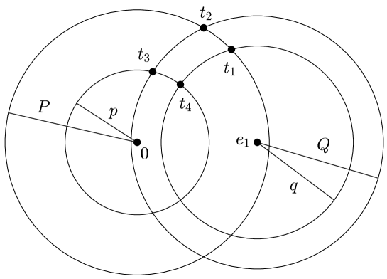
Figure 1: The four circles in Lemma 2.18.

2.18 Lemma.

Let $0<p<P$ and $0<q<Q$ be numbers such that $S(0,p)$ and $S(0,P)$ both intersect $S(e_{1},Q)$ at two points $t_{1},t_{2}$ and also $S(e_{1},q)$ at two points $t_{3},t_{4}$. Then the set

$$A\equiv(B^{2}(0,P)\setminus\bar{B}^{2}(0,p))\cap(B^{2}(e_{1},Q)\setminus\bar{B}^{2}(e_{1},q))\cap\mathbb{H}^{2}$$

does not meet the $e_{1}$-axis. Suppose that the points $t_{1},t_{2},t_{3},t_{4}$ occur in the positive order when we traverse $\partial A\,.$ Then

$$2\,\textnormal{diam}\,(A)\leq{\frac{\pi}{2}}(|t_{1}-t_{2}|+|t_{2}-t_{3}|+|t_{3}-t_{4}|+|t_{4}-t_{1}|)$$ (2.19)

and, moreover,

$$\begin{array}[]{l}|t_{1}-t_{2}|^{2}\leqslant P(Q^{2}-q^{2}),\vspace{0.5em}\\ |t_{2}-t_{3}|^{2}\leqslant Q(P^{2}-p^{2}),\vspace{0.5em}\\ |t_{3}-t_{4}|^{2}\leqslant p(Q^{2}-q^{2}),\vspace{0.5em}\\ |t_{4}-t_{1}|^{2}\leqslant q(P^{2}-p^{2}),\vspace{0.5em}\\ \textnormal{diam}\,(A)\leq 2\pi\max\{P,Q\}\sqrt{\varepsilon}\,.\end{array}$$

Proof.

It is clear that $2\,\textnormal{diam}\,(A)\leqslant L$, where $L$ is the sum of the lengths of the four circular arcs with endpoints $t_{i},t_{j}$. These four arcs form the boundary $\partial A$. For instance, the length of the first arc is less than $\frac{\pi}{2}|t_{1}-t_{2}|$ and similarly for other arcs and hence the desired bound (2.19) follows.

By Proposition 2.17 (1)

$$\begin{array}[]{ll}t_{1}=(a,\sqrt{P^{2}-a^{2}}),&\displaystyle a=\frac{1+P^{2}-q^{2}}{2},\vspace{0.5em}\\ t_{2}=(b,\sqrt{P^{2}-b^{2}}),&\displaystyle b=\frac{1+P^{2}-Q^{2}}{2},\vspace{0.5em}\\ t_{3}=(c,\sqrt{p^{2}-c^{2}}),&\displaystyle c=\frac{1+p^{2}-Q^{2}}{2},\vspace{0.5em}\\ t_{4}=(d,\sqrt{p^{2}-d^{2}}),&\displaystyle d=\frac{1+p^{2}-q^{2}}{2}.\end{array}$$

Next, we obtain by Proposition 2.17 (2)

$$\begin{array}[]{ll}|t_{1}-t_{2}|\leqslant\sqrt{|a-b|P}=\sqrt{P(Q^{2}-q^{2})},\vspace{0.5em}\\ |t_{2}-t_{3}|\leqslant\sqrt{|b-c|Q}=\sqrt{Q(P^{2}-p^{2})},\vspace{0.5em}\\ |t_{3}-t_{4}|\leqslant\sqrt{|c-d|p}=\sqrt{p(Q^{2}-q^{2})},\vspace{0.5em}\\ |t_{4}-t_{1}|\leqslant\sqrt{|a-d|q}=\sqrt{q(P^{2}-p^{2})}.\end{array}$$

The final inequality follows, because

$$|t_{1}-t_{2}|\leq\sqrt{P(Q+q)2\varepsilon}\leq 2m\sqrt{\varepsilon}\,,\quad m=\max\{P,Q\},$$

and similar upper bounds hold for each of the terms on the right hand side of (2.19). ∎

For $0<s<r$, $x\in\mathbb{R}^{n}\,,$ we denote $R(x,r,s)=B^{n}(x,r)\setminus\bar{B}^{n}(x,s)$.

2.20 Lemma.

Let $x\in\mathbb{H}^{2}$ with $|x|+|x-e_{1}|>1$,

$$\varepsilon\in(0,\min\{|x|+|x-e_{1}|-1,1-||x|-|x-e_{1}||\}/3)$$

and let

$$A(\varepsilon)=R(0,|x|+\varepsilon,|x|-\varepsilon)\cap R(e_{1},|x-e_{1}|+\varepsilon,|x-e_{1}|-\varepsilon)\cap{\mathbb{H}}^{2}\,.$$

Then

$$\textnormal{diam}\,(A(\varepsilon))\leqslant 2\pi\max\{|x|,|x-e_{1}|\}\sqrt{\varepsilon}\,.$$

Proof.

The bound for $\varepsilon$ implies that the condition $1>|u-v|$ in Lemma 2.18 is satisfied for $u=|x|\pm\varepsilon$ and $v=|x-e_{1}|\pm\varepsilon\,.$ The proof follows from Lemma 2.18. ∎

3 Diameter estimate

In this section we will consider the intersection of the two annuli

$$(B^{n}(0,b)\setminus\overline{B}^{n}(0,a))\cap(B^{n}(e_{1},d)\setminus\overline{B}^{n}(e_{1},c))\,,$$ (3.1)

when $b>a>0\,,d>c>0\,.$ In order to simplify the situation, we require that this intersection does not contain points of the $e_{1}$-axis. For this purpose we introduce a sufficient condition which we call the annuli intersection criterion. We apply this criterion to study a $K$-quasiconformal mapping $f\colon\overline{\mathbb{R}}^{n}\to\overline{\mathbb{R}}^{n}$ with $f(y)=y$ for $y\in\{0,e_{1},\infty\}$ and our goal is to find an upper bound for quantities such as $|f(x)-x|\,,$ when $K>1$ is small enough, the bound for $K$ depending on $n,$ $|x|,|x-e_{1}|$ in an explicit way via the annuli intersection criterion.

3.2.    The annuli intersection criterion ​​. We consider the region (3.1) and will give a criterion for the radii which ensures that this region (3.1) does not contain points of the $e_{1}$-axis. Without loss of generality we may assume here that $n=2\,.$ The crucial requirement is that given a pair of two boundary circles of the four boundary circles of the annuli in (3.1), these two circles have a point of intersection. Altogether there are four points of intersection, denoted $t_{1},t_{2},t_{3},t_{4}\,,$ which form the corner points of the region (3.1) :

$$(1)\quad\{t_{1}\}=S(0,b)\cap S(e_{1},c)\Rightarrow 1-c<b<1+c$$

$$(2)\quad\{t_{2}\}=S(0,b)\cap S(e_{1},d)\Rightarrow 1-d<b<1+d$$

$$(3)\quad\{t_{3}\}=S(0,a)\cap S(e_{1},d)\Rightarrow 1-d<a<1+d$$

$$(4)\quad\{t_{4}\}=S(0,a)\cap S(e_{1},c)\Rightarrow 1-c<a<1+c$$

We see that $(1)\Rightarrow(2)$ and $(4)\Rightarrow(3)$ because $0<c<d\,.$

Conclusion: For the desired intersection property, it is enough to require

$$1-c<a<1+c\quad\&\quad 1-c<b<1+c\,.$$ (3.3)

These inequalities constitute the annuli intersection criterion.

A geometric consequence of the annuli intersection criterion is that all the triangles $\Delta(0,1,t_{j}),j=1,2,3,4\,,$ are non-degenerate, i.e. that the strict triangle inequalities

$$|t_{j}|+|t_{j}-e_{1}|>1\,,\quad j=1,2,3,4\,,$$

$$1>||t_{j}|-|t_{j}-e_{1}||\,,\quad j=1,2,3,4$$

hold.

3.4.    Application of annuli intersection criterion ​​. Fix a point $x\in{\mathbb{R}^{n}}$ with $|x|+|x-e_{1}|>1\,.$ We will next find $\delta$ such that with

$$a=|x|-\delta,\quad b=|x|+\delta,\quad c=|x-e_{1}|-\delta,\quad d=|x-e_{1}|+\delta,$$

the annuli intersection criterion (3.3) is valid. Rewriting (3.3) with these $a,b,c,d$ shows that it is enough to choose

$$\delta<\min\{1-||x|-|x-e_{1}||,|x|+|x-e_{1}|-1\}/3\equiv\Delta(x)\,.$$ (3.5)

Note that $\Delta(x)\in(0,1/3)\,.$

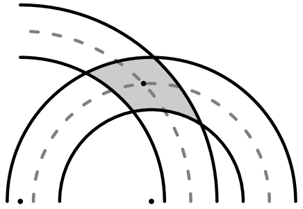
Figure 2: The shaded region is the cross-section of the set $A(\delta)$ in Theorem 3.6 (1) with a half-plane that contains both $0$ and $e_{1}$.

3.6 Theorem.

Fix $x\in\mathbb{R}^{n}\setminus\{0,e_{1}\}$ with $|x|+|x-e_{1}|>1$ and let $\Delta(x)$ be as in (3.5).

(1) If $\delta\in(0,\Delta(x))\,,$ then the intersection of annuli

$$A(\delta)\equiv(B^{n}(0,|x|+\delta)\setminus\overline{B}^{n}(0,|x|-\delta))\cap(B^{n}(e_{1},|x-e_{1}|+\delta)\setminus\overline{B}^{n}(e_{1},|x-e_{1}|-\delta))\,,$$

does not contain points of the $e_{1}$-axis. Moreover, if $\mathbb{H}=\{x\in\mathbb{R}^{n}:x_{2}>0,x_{3}=\dots=x_{n}=0\}\,,$ then

$$\textnormal{diam}\,(\mathbb{H}\cap A(\delta))\leq 2\pi\max\{|x|,|x-e_{1}|\}\sqrt{\delta}\,.$$

(2) If $\delta\in(0,\Delta(x))\,,$

$$1<K\leq 1+\left(\frac{\log(\delta/2+1)}{62}\right)^{2}<1+10^{-5}\,,$$

and $f\in QC_{K}(\mathbb{R}^{n})\,$ with $f(z)=z$ for $z\in\{0,e_{1}\}\,,$ then $f(x)\in A(\delta)\,.$ Moreover, there exists a Möbius transformation, a rotation $h:\mathbb{R}^{n}\to\mathbb{R}^{n}$ around the $e_{1}$-axis, such that

$$|h(f(x))-x|\leq 2\pi\max\{|x|,|x-e_{1}|\}\sqrt{\delta}\,.$$

Proof.

(1) Fix $z\in A(\delta)\,.$ The choice of $\Delta(x)$ implies $|z|+|z-e_{1}|>1\,$ and that the annuli intersection criterion (3.3) holds for $a=|x|-\varepsilon,b=|x|+\varepsilon,c=|x-e_{1}|-\varepsilon,d=|x-e_{1}|+\varepsilon\,.$ The upper bound for $\textnormal{diam}\,(\mathbb{H}\cap A(\delta))$ follows directly from Lemma 2.20.

(2) We need to prove that both

$$|x|-\delta\leq|f(x)|\leq|x|+\delta\quad\textrm{and}\quad|x-e_{1}|-\delta\leq|f(x)-e_{1}|\leq|x-e_{1}|+\delta$$

hold. It is enough to prove the first inequality because the proof of the second one is similar. Let us denote $l(x)=c_{3}^{-1}\min\{|x|^{\alpha},|x|^{\beta}\}$ and $u(x)=c_{3}\max\{|x|^{\alpha},|x|^{\beta}\}$ where $c_{3}=e^{60\sqrt{K-1}}$. Then by Proposition 2.5

$$l(x)\leq|f(x)|\leq u(x)$$

for all $x\in{\mathbb{R}^{n}}\,.$

We will first consider the case $0<|x|<1$. By Lemma 2.11

$$\max\{u(x)-|x|,|x|-l(x)\} = \max\left\{c_{3}|x|^{\alpha}-|x|,|x|-\frac{1}{c_{3}}|x|^{\beta}\right\}$$

$$= c_{3}|x|^{\alpha}-|x|$$

$$\leq \exp(60\sqrt{K-1})|x|^{\alpha}-|x|$$

$$\leq \exp(60\sqrt{K-1})|x|^{1/K}-|x|$$

$$\leq \exp(60\sqrt{K-1})-1.$$

Now $\exp(60\sqrt{K-1})-1\leq\delta$ is equivalent to

$$K\leq\left(\frac{\log(\delta+1)}{60}\right)^{2}+1.$$ (3.7)

If $|x|=1$, then

$$\max\{u(x)-|x|,|x|-l(x)\}=c_{3}-1$$

and therefore we want $\exp(60\sqrt{K-1})-1\leq\delta$, which is equivalent to

$$K\leq\left(\frac{\log(\delta+1)}{60}\right)^{2}+1.$$ (3.8)

Let us then consider the case $1<|x|<2$. By Lemma 2.11

$$\max\{u(x)-|x|,|x|-l(x)\} = \max\left\{c_{3}|x|^{\beta}-|x|,|x|-\frac{1}{c_{3}}|x|^{\alpha}\right\}$$

$$= c_{3}|x|^{\beta}-|x|$$

$$\leq \exp(60\sqrt{K-1})|x|^{\beta}-|x|$$

$$\leq \exp(60\sqrt{K-1})|x|^{K}-|x|$$

$$\leq |x|(\exp(60\sqrt{K-1})|x|^{K-1}-1)$$

$$\leq 2(\exp(60\sqrt{K-1}+(K-1)\log|x|)-1)$$

$$\leq 2(\exp(62\sqrt{K-1})-1).$$

Now $2(\exp(62\sqrt{K-1})-1)\leq\delta$ is equivalent to

$$K\leq\left(\frac{\log(\delta/2+1)}{62}\right)^{2}+1.$$ (3.9)

By combining (3.7), (3.8) and (3.9) we have

$$|x|-\delta\leq l(x)\leq|f(x)|\leq u(x)\leq|x|+\delta$$

for

$$K \leq \min\left\{\left(\frac{\log(\delta+1)}{60}\right)^{2}+1,2,\left(\frac{\log(\delta/2+1)}{62}\right)^{2}+1\right\}$$

$$= \min\left\{\left(\frac{\log(\delta/2+1)}{62}\right)^{2}+1,2\right\}=1+\left(\frac{\log(\delta/2+1)}{62}\right)^{2}<1+10^{-5}\,.$$

A similar argument also implies $|x-e_{1}|-\delta\leq|f(x)-e_{1}|\leq|x-e_{1}|+\delta$ and the assertion follows. Finally, the rotation $h$ is taken to be the rotation around the $e_{1}$-axis mapping $f(x)$ to the plane determined by the $e_{1}$-axis and the point $x\,.$ ∎

4 The main results

In this section we will apply the diameter estimates to obtain results for distortion results in terms of the $j$-metric and the quasihyperbolic metric. For the convenience of the reader we recall some basic properties of this metric. For a given pair of points $x,y\in G,$ the infimum in (1.4) is always attained [GO], i.e., there always exists a quasihyperbolic geodesic $J_{G}[x,y]$ which minimizes the quasihyperbolic length, $k_{G}(x,y)=\ell_{k}(J_{G}[x,y])\,$ and furthermore the distance is additive on the geodesic: $k_{G}(x,y)=$ $k_{G}(x,z)+k_{G}(z,y)$ for all $z\in J_{G}[x,y]\,.$

4.1 Lemma.

([Vu1, Lemma 3.7 (2)], [GP, Lemma 2.1]) . Fix $\lambda\in(0,1)\,.$ For $x,y\in G={\mathbb{R}}^{n}\setminus\{0\}$ with $|x-y|\leq\lambda|x|$ we have

$$j_{G}(x,y)\leq k_{G}(x,y)\leq c_{1}(\lambda)j_{G}(x,y)$$

with $c_{1}(\lambda)=1/(1-\lambda).$

Only in rare special cases there is a formula for the quasihyperbolic distance between two points. One such case is when $x,y\in G={\mathbb{R}}^{n}\setminus\{0\}\,.$ Martin and Osgood [MO] proved that

$$k_{G}(x,y)=\sqrt{\log^{2}\frac{|x|}{|y|}+\left(2\,\mathrm{arcsin}\left(\frac{1}{2}\left(\left|\frac{x}{|x|}-\frac{y}{|y|}\right|\right)\right)\right)^{2}}\,,$$ (4.2)

for all $x,y\in G\,.$

Proof of Theorem 1.2.

The proof follows from Theorem 3.6. ∎

We now prove Theorem 1.3, which can be easily generalized for arbitrary subdomains of $\mathbb{R}^{n}\,.$

Proof of Theorem 1.3.

Both sides of the claim are invariant under a homothety mapping $z\mapsto tz,t>0,$ and so is the normalization. Moreover, composition with a homothety does not change $K$-quasiconformality. Therefore we may assume that $x=e_{1},f(e_{1})=e_{1}\,$ and by symmetry we, furthermore, assume that $|y|\geq 1$. Now

$$\frac{|f(y)-f(e_{1})|}{|f(e_{1})|}=|f(y)-f(e_{1})|\leq\eta\left(|e_{1}-y|\right)$$

and

$$\frac{|f(y)-f(e_{1})|}{|f(y)|}=\frac{|f(y)-f(e_{1})|}{|f(y)-f(0)|}\leq\eta\left(\frac{|e_{1}-y|}{|y-0|}\right)=\eta\left(\frac{|e_{1}-y|}{|y|}\right).$$

Therefore by Proposition 2.5 and Lemma 2.14 (4)

$$j(f(e_{1}),f(y)) = \log\left(1+\frac{|f(e_{1})-f(y)|}{\min\{|f(e_{1})|,|f(y)|\}}\right)$$

$$\leq \log\left(1+\max\left\{\eta(|y-e_{1}|),\eta\left(\frac{|x-y|}{|y|}\right)\right\}\right)$$

$$= \log(1+\eta(|y-e_{1}|))$$

$$\leq \log(1+c_{3}\max\{|y-e_{1}|^{\alpha},|y-e_{1}|^{1/\alpha}\})$$

$$\leq \left\{\begin{array}[]{ll}c_{3}\log^{\alpha}(1+|y-e_{1}|),&0<|y-e_{1}|<1,\\ \frac{c_{3}}{\alpha}\log(1+|y-e_{1}|),&|y-e_{1}|\geq 1.\end{array}\right.$$

By choosing $c(K)=c_{3}/\alpha$, where $c_{3}=\exp(60\sqrt{K-1})$ is as in Lemma 2.11, we have $c(K)\to 1$ as $K\to 1$ and the assertion follows. ∎

4.4 Corollary.

Let $G\subset\mathbb{R}^{n}$ be a domain, $f\in QC_{K}(\mathbb{R}^{n})$, $K\in(1,2]$ and $f(z)=z$ for all $z\in\partial G$. There exists $c(K)$ such that for all $x,y\in G$

$$j_{G}(f(x),f(y))\leq c(K)\max\{j_{G}(x,y)^{\alpha},j_{G}(x,y)\},$$

where $\alpha=K^{1/(1-n)}$, and $c(K)\to 1$ as $K\to 1$.

Proof.

We may assume $0,e_{1}\in\partial G$ and $d(x)=|x|\leq d(y)\leq|y|$. Now for $z\in\partial G$

$$\frac{|f(y)-f(x)|}{|z-f(x)|}=\frac{|f(y)-f(x)|}{|f(z)-f(x)|}\leq\eta\left(\frac{|x-y|}{|z-x|}\right)\leq\eta\left(\frac{|x-y|}{|x|}\right)$$

and

$$\frac{|f(y)-f(x)|}{|z-f(y)|}=\frac{|f(y)-f(x)|}{|f(z)-f(y)|}\leq\eta\left(\frac{|x-y|}{|z-y|}\right)\leq\eta\left(\frac{|x-y|}{|y|}\right)\leq\eta\left(\frac{|x-y|}{|x|}\right).$$

Therefore by Proposition 2.5 and Lemma 2.14 (4)

$$j(f(x),f(y)) = \log\left(1+\frac{|f(x)-f(y)|}{\displaystyle\min_{z\in\partial G}\{|f(x)-z|,|f(y)-z|\}}\right)$$

$$\leq \log\left(1+\eta\left(\frac{|y-x|}{|x|}\right)\right)$$

$$\leq \log\left(1+c_{3}\max\left\{\frac{|y-x|^{\alpha}}{|x|^{\alpha}},\frac{|y-x|^{1/\alpha}}{|x|^{1/\alpha}}\right\}\right)$$

$$\leq \left\{\begin{array}[]{ll}c_{3}\log^{\alpha}\left(1+\frac{|y-x|}{|x|}\right),&0<|y-x|<1,\\ \frac{c_{3}}{\alpha}\log\left(1+\frac{|y-x|}{|x|}\right),&|y-x|\geq 1.\end{array}\right.$$

By choosing $c(K)=c_{3}/\alpha$, where $c_{3}=\exp(60\sqrt{K-1})$ is as in Lemma 2.11, we have $c(K)\to 1$ as $K\to 1$ and the assertion follows. ∎

Proof of Theorem 1.6.

Fix $\lambda\in(0,1/2)\,.$ Let $c\geq 1$ be the constant of Theorem 1.3 and write

$$\mu(\lambda)=\frac{1}{c}\min\{\log(1/(1-\lambda)),\log^{\beta}(1/(1-\lambda))\}=\frac{1}{c}\log^{\beta}(1/(1-\lambda))\,,\quad\beta=1/\alpha\,.$$

Note that $c\to 1$ when $K\to 1\,.$ The rest of the proof is now divided into two cases.

Case A. $k_{G}(x,y)\leq\mu(\lambda)\,.$ By Theorem 1.3 and Lemma 4.1 we have

$$\frac{|f(x)-f(y)|}{|f(x)|} \leq \exp\left({c}\max\{j_{G}(x,y)^{\alpha},j_{G}(x,y)\}\right)-1$$ (4.6)

$$\leq \exp\left({c}\max\left\{\frac{\log^{\beta}(1/(1-\lambda))}{c},\frac{\log(1/(1-\lambda))}{c}\right\}\right)-1$$

$$= \lambda/(1-\lambda)\,.$$

Therefore we can use Lemma 4.1 and Theorem 1.3 to find an upper bound for $k_{G}(f(x),f(y))$ in terms of $k_{G}(x,y)$ and $\lambda$. By Lemma 4.1, (4.6), and Theorem 1.3 we have

$$k_{G}(f(x),f(y)) \leq c_{1}(\lambda)j_{G}(f(x),f(y))\leq cc_{1}(\lambda)\max\{j_{G}(x,y)^{\alpha},j_{G}(x,y)\}$$

$$\leq cc_{1}(\lambda)\max\{k_{G}(x,y)^{\alpha},k_{G}(x,y)\}\,.$$

Case B. $k_{G}(x,y)\geq\mu(\lambda)\,.$ Choose points $x_{j},j=0,...,p+1,$ on the quasihyperbolic geodesic segment $J_{G}[x,y]$ joining $x$ with $y$ such that $x_{0}=y,x_{p+1}=x$ and $k_{G}(x_{j+1},x_{j})=\mu(\lambda)$ for $j=0,...,p-1\,,$ $k_{G}(x_{p+1},x_{p})\leq\mu(\lambda)\,.$ Because the quasihyperbolic distance is additive on the geodesic we see that

$$k_{G}(x,y)=\sum_{j=0}^{p}k_{G}(x_{j+1},x_{j})\geq p\mu(\lambda)\Rightarrow p\leq k_{G}(x,y)/\mu(\lambda)\,.$$

Next, by the triangle inequality and by Case A

$$k_{G}(f(x),f(y))\leq\sum_{j=0}^{p}k_{G}(f(x_{j+1}),f(x_{j}))\leq cc_{1}(\lambda)\sum_{j=0}^{p}k_{G}(x_{j+1},x_{j})^{\alpha}=V\,.$$

Next, using the property of weighted mean values [M, p. 76, Theorem 1]

$$\sum_{j=0}^{p}u_{j}^{\alpha}\leq(p+1)^{1-\alpha}\left(\sum_{j=0}^{p}u_{j}\right)^{\alpha}\,\textrm{ for\, all \, positive}\,\,u_{j}$$

we have

$$V \leq cc_{1}(\lambda)(p+1)^{1-\alpha}\left(\sum_{j=0}^{p}k_{G}(x_{j+1},x_{j})\right)^{\alpha}$$

$$\leq cc_{1}(\lambda)\mu(\lambda)^{\alpha-1}\left(1+\frac{\mu(\lambda)}{k_{G}(x,y)}\right)^{1-\alpha}k_{G}(x,y)$$

$$\leq cc_{1}(\lambda)\mu(\lambda)^{\alpha-1}2^{1-\alpha}k_{G}(x,y)\,.$$

In view of the above Cases A and B we see that in both cases we have the claim with the constant

$$\omega(K,n)=cc_{1}(\lambda)\mu(\lambda)^{\alpha-1}2^{1-\alpha}\,.$$

It remains to prove that $\omega(K,n)\to 1$ when $K\to 1\,.$ It suffices to show that we can choose $\lambda$ depending on $K,n$ such that

$$\mu(\lambda)^{\alpha-1}=c^{1-\alpha}\log^{1-\beta}(1/(1-\lambda))\to 1$$

when $K\to 1\,.$ For instance the choice $\lambda=\beta-1$ will do. ∎

Agard and Gehring have studied the angle distortion under quasiconformal mappings of the plane [AG]. Motivated by their work we record the following corollary of Theorem 1.6.

4.7 Corollary.

Suppose that under the hypotheses of Theorem 1.6 $x,y\in S^{n-1}$ and $f(x),f(y)\in S^{n-1}$ and let $\phi$ and $\psi$ be the angles between the segments $[0,x],[0,y]$ and $[0,f(x)],[0,f(y)]\,,$ respectively. Then

$$\psi\leq\omega(K,n)\max\{\phi^{\alpha},\phi\}\,.$$

Proof.

The proof follows easily from the Martin-Osgood formula (4.2) . ∎

4.8 Remark.

It is well-known (see [LVV],[AVV2, Lemma 4.28]) that for a given $K\geq 1$ there exists a $K$-quasiconformal mapping $f\colon\mathbb{R}^{n}\to\mathbb{R}^{n}$ with $f(0)=0$ such that $f(-e_{1})=-e_{1}$ and $f(e_{1})=\lambda(K^{1/(n-1)})e_{1}$, where $\lambda(K)=\varphi_{K}(1/\sqrt{2})^{2}/(1-\varphi_{K}(1/\sqrt{2})^{2})$ (see [AVV1, p. 203, 204]). Choosing $G=\mathbb{R}^{n}\setminus\{0\}$ and $x=1=-y$ in Theorem 1.3 we see that

$$\log(1+L)\leq c(K)\log 3,$$

where $L=(1+\lambda(K^{1/(n-1)}))$, and hence the constant $c(K)$ has to satisfy

$$c(K)\geq\frac{\log(2+\lambda(K^{1/(n-1)}))}{\log 3}.$$

In order to compare this estimate to the upper bound in Theorem 1.3 well-known estimates for $\lambda(K^{1/(n-1)})$ may be used. For instance we know that $\lambda(K)\geq\exp(\pi(K-1))$ by [AVV1, Corollary 10.33].

This same idea can be applied to produce a lower bound for the constant $\omega(K,n)$ of Theorem 1.6 as well.

Acknowledgement. The second author wishes to acknowledge the suggestions offered by Vladimir Bozin.

Appendix A Appendix: Bernoulli type inequalities

In Lemma 2.14 we introduced Bernoulli type inequalities. In this appendix we introduce some additional Bernoulli type inequalities.

A.1 Lemma.

Let $0<a\leq 1\leq b$ and $\varphi(t)=\max\{t^{a},t^{b}\}$. Then, with $u=\log^{1-a}2$, $v=\log^{1-b}2$,

• For $t\in(0,\infty)$

  $$f_{3}(t)=\frac{\log(1+t^{b})}{\log^{b}(1+t)}\leq v.$$

  The function $f_{3}(t)$ is increasing on $(0,1)$ and decreasing on $(1,\infty)$ with $f_{3}(1)=v$.

• For $t\in(0,\infty)$

  $$v^{-1}\log(1+\varphi(t))\leq\varphi(\log(1+t)).$$

• For $t\in(0,\infty)$

  $$\varphi(\log(1+t))\leq\left\{\begin{array}[]{ll}u^{-1}\log(1+\varphi(t)),&t\in(0,e-1],\\ \log^{b}(1+\varphi(t)),&t>e-1.\end{array}\right.$$

• For $t\in(0,t_{0})$, $t_{0}>0$ and

  $$f_{8}(t)=\frac{\log(1+\varphi(t))}{\varphi(\log(1+t))}$$

  we have $\min\{u,f(t_{0})\}\leq f(t)\leq\log(1+(e-1)^{b})$.

• For $s,t>0$

  $$2^{1-b}\leq\frac{\varphi(s)+\varphi(t)}{\varphi(s+t)}\leq 2^{1-a}.$$

Proof.

(1) Follows from Lemma 2.14 (2) by choosing $b=1/a$.

(2) If $t\in(0,1]$ then by Lemma 2.14 (2)

$$\log(1+\varphi(t))=\log(1+t^{a})\leq\log^{a}(1+t)=\varphi(\log(1+t))$$

and if $t\in[1,e-1]$ then by (1)

$$\log(1+\varphi(t))=\log(1+t^{b})\leq v\log^{b}(1+t)\leq v\log^{a}(1+t)=v\varphi(\log(1+t)).$$

If $t\geq e-1$ then by (1)

$$\log(1+\varphi(t))=\log(1+t^{b})\leq v\log^{b}(1+t)=v\varphi(\log(1+t))$$

and the assertion follows.

(3) If $t\in(0,1]$ then by Lemma 2.14 (2)

$$\varphi(\log(1+t))=\log^{a}(1+t)\leq u^{-1}\log(1+t^{a})=u^{-1}\log(1+\varphi(t)).$$

and if $t\in[1,e-1]$ then by Lemma 2.14 (2)

$$\varphi(\log(1+t))=\log^{a}(1+t)\leq u^{-1}\log(1+t^{a})\leq u^{-1}\log(1+t^{b})=u^{-1}\log(1+\varphi(t)).$$

If $t\geq e-1$ then by (1)

$$\varphi(\log(1+t))=\log^{b}(1+t)\leq\log^{b}(1+t^{b})=\log^{b}(1+\varphi(t)).$$

and the assertion follows.

(4) For $t\in(0,1]$, Lemma 2.14 (2) implies that $u\leq f(t)\leq 1$ and for $t\geq e-1$, (1) implies that $f(t_{0})\leq f(t)\leq f(e-1)=\log(1+(e-1)^{b})$.

Let us consider the case $t\in(1,e-1)$. Now $f^{\prime}(t)\geq 0$ is equivalent to

$$\frac{\log(1+t^{b})}{\log(1+t)}\leq\frac{b(1+t)}{at(1+t^{-b})}.$$ (A.2)

We have

$$\frac{\log(1+t^{b})}{\log(1+t)}\leq b\leq\frac{b(1+t)}{t(1+t^{b})}\leq\frac{b(1+t)}{at(1+t^{-b})},$$

where the first inequality follows from Lemma 2.14 (1) and the second inequality holds, because $t(1+t^{-b})\leq 1+t$ is equivalent to $t^{1-b}\leq 1$ which holds true by the selection of $b$ and $t$. Now (A.2) holds and $f(t)$ is increasing on $(1,e-1)$. Thus $u=f(1)\leq f(t)\leq f(e-1)$. The assertion follows by combining the three cases.

(5) Follows from [AVV1, 1.58 (27) p. 340]. ∎

(Riku Klén, Matti Vuorinen) Department of Mathematics and Statistics, University of Turku, 20014 Turku, Finland

E-mail address: riku.klen@utu.fi, vuorinen@utu.fi

(Vesna Todorčević) Mathematical Institute of the Serbian Academy of Sciences and Arts, Faculty of Organizational Sciences, University of Belgrade, Serbia

E-mail address: vesnat@fon.bg.ac.rs

References

[AG]S. B. Agard and F.W. Gehring:Angles and quasiconformal mappings. Proc. London Math. Soc. (3) 14a 1965 1–21.
[AVV1]G.D. Anderson, M.K. Vamanamurty, and M. Vuorinen:
Conformal Invariants, Inequalities and Quasiconformal Maps. John Wiley & Sons, 1997.
[AVV2]G.D. Anderson, M.K. Vamanamurty, and M. Vuorinen:
Sharp distortion theorems for quasiconformal mappings. Trans. Amer. Math. Soc. 305
(1988), 95–111.
[BGRT]M. Badger, J.T. Gill, S. Rohde and T. Toro:Quasisymmetry and Rectifiability of Quasispheres. Trans. Amer. Math. Soc. 366 (2014), no. 3, 1413–1431.
[BTCT]B. Bonfert-Taylor, R. Canary and E.C. Taylor:Quasiconformal Homogeneity after Gehring and Palka. Comput. Methods Funct. Theory 14 (2014), no. 2, 417–430.
[GL]F.P. Gardiner and N. Lakic:A vector field approach to mapping class actions.
Proc. London Math. Soc. (3) 92 (2006), no. 2, 403–427.
[GO]F.W. Gehring and B.G. Osgood:Uniform domains and the quasi-hyperbolic metric.
J. Anal. Math. 36 (1979), 50–74.
[GP]F.W. Gehring and B.P. Palka:Quasiconformally homogeneous domains. J. Anal. Math. 30 (1976), 172–199.
[KL]L. Keen and N. Lakic:
Hyperbolic geometry from a local viewpoint. London Math. Soc. Student Texts 68, Cambridge University Press, Cambridge, 2007.
[KMSV]R. Klén, V. Manojlović, S. Simić and M. Vuorinen:
Bernoulli inequality and hypergeometric functions. Proc. Amer. Math. Soc. 142 (2014) 559–573.
[LVV]O. Lehto, K.I. Virtanen, and J. Väisälä:Contributions to the distortion theory of quasiconformal mappings. Ann. Acad. Sci. Fenn. Ser. AI 273 (1959), 1–14.
[MV]V. Manojlović and M. Vuorinen:
On quasiconformal mappings with identity boundary values.
Trans. Amer. Math. Soc. 363 (2011), 2467–2479.
[MO]G.J. Martin and B.G. Osgood:
The quasihyperbolic metric and the associated estimates on the hyperbolic metric. J. Anal. Math. 47 (1986), 37–53.
[M]D. S. Mitrinović: Analytic inequalities. In
cooperation with P. M. Vasić. Die Grundlehren der mathematischen
Wissenschaften, Band 165 Springer-Verlag, New York-Berlin 1970.
[P]I. Prause:
Flatness properties of quasispheres. Comput. Methods Funct. Theory 7 (2007), no. 2, 527–541.
[R]Yu. G. Reshetnyak:
Stability theorems in geometry and analysis. Translated from the 1982 Russian original by N. S. Dairbekov and V. N. Dyatlov, and revised by the author. Translation edited and with a foreword by S. S. Kutateladze. Mathematics and its Applications, 304. Kluwer Academic Publishers Group, Dordrecht, 1994.
[S]P. Seittenranta:
Linear dilatation of quasiconformal maps in space. Duke Math. J. 91 (1998), no. 1, 1–16.
[T]O. Teichmüller: Ein Verschiebungssatz der quasikonformen
Abbildung.
(German) Deutsche Math. 7, (1944). 336–343. see also Teichmüller,
Oswald Gesammelte Abhandlungen. (German) [Collected papers] Edited
and with a preface by Lars V. Ahlfors and Frederick W. Gehring.
Springer-Verlag, Berlin-New York, 1982.
[V1]J. Väisälä:Lectures on
-dimensional quasiconformal mappings. Lecture Notes in
Mathematics, Vol. 229. Springer-Verlag, Berlin-New York, 1971.