Improving Wang-Landau sampling with adaptive windows

Abstract

Wang-Landau sampling (WLS) of large systems requires dividing the energy range into “windows” and joining the results of simulations in each window. The resulting density of states (and associated thermodynamic functions) are shown to suffer from boundary effects in simulations of lattice polymers and the five-state Potts model. Here, we implement WLS using adaptive windows. Instead of defining fixed energy windows (or windows in the energy-magnetization plane for the Potts model), the boundary positions depend on the set of energy values on which the histogram is flat at a given stage of the simulation. Shifting the windows each time the modification factor $f$ is reduced, we eliminate border effects that arise in simulations using fixed windows. Adaptive windows extend significantly the range of system sizes that may be studied reliably using WLS.

In recent years Wang-Landau sampling (WLS) landau ; landaupre ; wanglandau_other ; wang_landau_ajp has become an important algorithm for Monte Carlo (MC) simulations, and is being applied to a vast array of models in statistical physics and beyondwang_landau_ajp . WLS uses a random walk in energy ($E$) space to estimate the density of states, $g(E)$; to sample well the full range of energies, the walk is adjusted to spend approximately equal time intervals at each energy value. The estimate for $g(E)$ is refined successively, in a series of random walks. WLS has been used, for example, to simulate polymers 3d ; jain ; rampf_binder_paul ; parsons_williams and proteins rathore ; wuest_landau and to calculate the joint density of states (JDOS) of two or more variableszhouetal , e.g., $g(E,M)$ of magnetic systems ($M$ is the magnetization).

For models with a complex energy landscape, WLS permits simulation of larger systems than can be studied using conventional MC approaches. Because sampling the full range of energies of a large system is not viable using a single walk, one divides the energy range into slightly overlapping subintervals (“windows”) and samples each separately. The density of states $g(E)$ for the full energy range is then obtained via a matching procedure that consists of multiplying $g(E)$ in each window by a factor to force continuity of this function at the borders. (This yields $g(E)$ to within an overall multiplicative factor, permitting evaluation of canonical averages. If the absolute density of states is needed, the normalization must use some reference value for which the density of states is known exactly, for example, the ground state degeneracy.)

The question naturally arises whether sampling restricted to windows yields reliable estimates for $g(E)$, near the boundary energy values. Wang and Landau suggested that boundary effects would be negligible if adjacent windows were defined with a suitably large overlap landaupre . On the other hand, Schulz et al.schulz found it advantageous to introduce an additional rule, namely, whenever a configuration is rejected because its energy is greater than the maximum value, $E_{>}$, of a given window, one should update $g(E)$ for the current energy value. These prescriptions are effective for Ising models but do not eliminate boundary effects in all instances, e.g., in simulations of polymers preprint and systems where the JDOS is required shan .

Here we present an implementation of WLS that eliminates border effects. For the sake of clarity, we consider two examples with severe border problems: a lattice polymer with attractive interactions between nonbonded nearest-neighbor monomers baumgartner ; 3d ; douglas_ishinabe , simulated via reptationlandau_binder , and the calculation of $g(E,M)$ in the five-state Potts model fywu on the square lattice. (We note that while the reptation method is not suitable for sampling the most compact configurations, this limitation does not affect the conclusions presented here.)

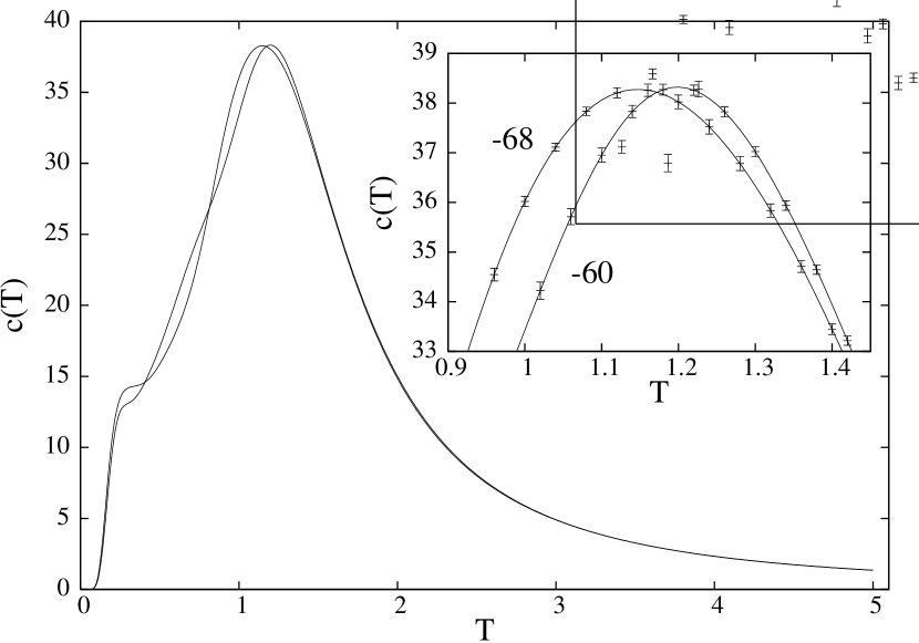
Figure 1: Specific heat of a polymer of $N=100$ monomers on the square lattice, using two windows and border energies $E_{b}$ = -68 and -60. The inset shows the neighborhood of the maximum. Average values and uncertainties are calculated using ten independent runs.

To begin, we document the border effects that arise in fixed-window simulations of polymers, focusing on the specific heat $c(T)$ (calculated as usual from the variance of the energy). The polymer chain is modeled as a self-avoiding walk on the square lattice. The energy is $E=-N_{nb}$, with $N_{nb}$ the number of nearest-neighbor contacts between nonconsecutive monomers. Our simulations sample the entire energy range, from the ground state $E_{min}$ to $E_{max}=0$. We encounter strong border effects, even if, following the suggestion of Ref. schulz , we use three overlapping levels at the border(s). Varying the border energy $E_{b}$, we find that the temperature $T_{m}$ at which $c(T)$ takes its maximum varies in an analogous manner (a smaller $E_{b}$ corresponds to a smaller $T_{m}$), signaling a systematic error (see Fig. 1). Evidently WLS using fixed windows yields distorted results for $g(E)$ in this system. (We stress that such a distortion does not arise in WLS of the 2d Ising model landaupre , for which simulations using fixed windows have been performed on lattices of up to $256\times 256$ sites.)

We shall now describe a procedure that eliminates the boundary effects described above. Recall first that in WLS, the simulation begins with an arbitrary configuration, and with $g(E)=1$ for all values of energy $E$. A random walk in energy space is realized by generating trial configurations and accepting them with probability $p(E_{1}\rightarrow E_{2})=\min(g(E_{1})/g(E_{2}),1)$, where $E_{1}$ is the current energy value and $E_{2}$ the energy of the trial configuration ${\cal C}_{2}$. If ${\cal C}_{2}$ is accepted, we update $g(E_{2})\rightarrow f\times g(E_{2})$ and $H(E_{2})\rightarrow H(E_{2})+1$; otherwise, $g(E_{1})\rightarrow f\times g(E_{1})$ and $H(E_{1})\rightarrow H(E_{1})+1$, where the histogram $H(E)$ records the number of visits to energy $E$, and $f$ is the modification factor, initially set to $e=2.71828\ldots$. When $H(E)$ is sufficiently flat, it is reset to zero and a new random walk is initiated, with a smaller $f$, e.g., $f\rightarrow\sqrt{f}$, used to update $g(E)$. The simulation ends when $f$ is sufficiently close to $1$, e.g., $f\approx 1+10^{-6}$.

The histogram is said to be flat if, for all energies in the window of interest, $H(E)>\kappa\overline{H}$, where the overline denotes an average over energies. (Typically, $\kappa=0.8$, as used here.) In WLS with fixed windows, this stopping criterion is applied in each window. In our method, by contrast, we determine the range over which the histogram has attained the desired degree of uniformity at various stages of the simulation.

Initially, we allow the WLS random walk to visit all possible energies $E_{min}\leq E\leq E_{max}$, accumulating the histogram in the usual manner. After a certain number $N_{1}$ of Monte Carlo steps (in practice we use $N_{1}=10^{4}$), we check if the histogram, restricted to the interval $E_{w}\leq E\leq E_{max}$, is flat. (Here $E_{w}=E_{max}-W$, with $W$ defining the minimum acceptable window size.) If it is not flat, we perform an additional $N_{1}$ Monte Carlo steps, and check again, repeating until the histogram is flat on the minimal window. Once this condition is satisfied, we check whether the existing histogram is in fact flat on a larger window. (This is done by including the energy level just below $E_{w}$ in $\overline{H}$ and checking if the flatness criterion, $H(E)>\kappa\overline{H}$, holds in the enlarged window. In this manner, adding levels one by one, we identify the largest window over which flatness is satisfied.) Let $E^{*}\leq E_{w}$ be the smallest energy such that the histogram, restricted to the interval $[E^{*},E_{max}]$, is flat, and let $E_{1}=E^{*}+\Delta E$, where $\Delta E$ determines the overlap between adjacent windows. In the next stage of the simulation, we restrict the random walk to energies $E_{min}\leq E\leq E_{1}+\Delta E$. After $N_{1}$ steps we check if the histogram is flat on the interval $[E_{1}+\Delta E-W,E_{1}+\Delta E]$, and proceed as above, until all possible energies have been included in a window with a flat histogram (see Fig. 2). To avoid problems that might arise with very small windows, the final window (with lower limit $E_{min}$) always has a width $\geq W$. In the studies shown below we use $W=(E_{max}-E_{min})/10$ and $\Delta E=3$ for lattice polymers ($\Delta E=1$ or $\Delta M=1$ for the Potts model). Once all allowed energies have been sampled, we connect the functions $g(E)$ associated with the various windows by imposing continuity at $E_{1}$, $E_{2}$,…,$E_{n}$. Then the entire procedure is repeated using the next value of the modification factor $f$, that is, $f\to\sqrt{f}$; the simulation ends once $f-1<10^{-6}$.

Figure 2: Lower panel: schematic of adaptive windows; the value of $E_{max}$ depends on the model, while $\Delta E$ is chosen to ensure sufficient overlap. $E^{*}$ and $E_{1}$, $E_{2}$, etc., are determined during the simulation not fixed beforehand. Upper panel: example of a histogram and associated window in the lattice polymer simulation.

Note that at each iteration (using a different value of $f$), the borders $E_{j}$ are chosen differently: repetition of a border value in successive iterations is prohibited. This point is crucial to the functioning of our method; if the borders were fixed, errors incurred at a given iteration (similar to those seen in Fig. 1) would accumulate, rather than being corrected in subsequent iterations. (Here it is well to remember that WLS functions precisely because errors in $g(E)$ incurred at a given value of $f$ tend to be corrected at subsequent stages.)

Figure 3: Density of states $g(E)$ of two-dimensional polymers, $N=200$. Solid line: adaptive-window sampling; dashed line: Metropolis sampling, using the ratios $g(E)/g(E_{ref})$. Circles denote the limits of the energy ranges associated with each temperature in Metropolis sampling.

It is important to stress that energy windows are not merely a device for accelerating the simulation, but are in fact necessary in studies of large systems; without them, WLS simply does not converge. Thus, the largest lattice polymer we are able to study without windows is $N=70$; using the adaptive-window scheme, studies including the entire range of energies are possible on chains of at least 300 monomers. To test the validity of our method, we compare $g(E)$ (for $N=200$), given by our scheme with that obtained using high-resolution Metropolis Monte Carlolandau_binder ; excellent agreement is found (see Fig. 3). (Metropolis simulations are performed at temperatures $T=1.0,1.5,3.0$ and $10.0$, using $10^{8}$ MC steps per study, using the RAN2 random number generator numericalrecipes . In Metropolis MC, the expected number $m(E)$ of visits to energy $E$ satisfies $m(E)/m(E_{ref})=e^{-(E-E_{ref})/k_{B}T}g(E)/g(E_{ref})$. We use this relation to determine the ratios $g(E)/g(E_{ref})$, by equating $m(E)$ to the actual number of visits to energy $E$ during the simulation. At each temperature, a certain range of energies are well sampled; for each temperature studied, we take the reference energy $E_{ref}$ as the most visited value. The resulting values for $g(E)$ are normalized by equating $g(E_{ref})$ to the corresponding value obtained via WLS.)

We turn now to the $Q$-state Potts modelfywu , with Hamiltonian

$${\cal H}=-J\sum_{\langle ij\rangle}\delta_{\sigma_{i},\sigma_{j}}-h\sum_{i}\delta_{\sigma_{i},1}$$ (1)

where $\sigma_{i}=1,2,...,Q$; $\langle ij\rangle$ denotes pairs of nearest-neighbor spins, $J>0$ is a ferromagnetic coupling, and $h$ is an external field that couples to one of the states. (Our units are such that $J/k_{B}=1$.) We use WLS with a 2d random walk to determine the JDOS $g(E,M)$. [Here $E=-\sum_{\langle ij\rangle}\delta_{\sigma_{i},\sigma_{j}}$ and $M=\sum_{i}\delta_{\sigma_{i},1}$. Using $g(E,M)$, thermodynamic properties may be obtained for arbitrary $(T,h)$.] We study the five-state model on square lattices of 32 $\times$ 32 sites with periodic boundaries; we use the R1279 shift register random number generator landau_binder .

We tried to parallelize the 2d WLS by performing independent random walks on overlapping $(E,M)$ regions. We divided the parameter space into strips with: (i) restricted values of $E$ and unrestricted $M$; (ii) restricted $M$ and unrestricted $E$; and (iii) rectangles with both $E$ and $M$ restricted. The independent random walks were carried out in parallel and the densities of states from adjacent regions were normalized at a single common $(E,M)$ point, or by minimizing the least-square distance between an overlapping $(E,M)$ region. We found, however, that the resulting density of states exhibits some small discontinuities which affect the probability distributions of energy and magnetization, as illustrated by the dashed line in Fig.4 for $P(M,T,h)$ for the case (ii) above. This curve was obtained with one simulation (hence no error bars are displayed); the temperature is taken such that $P(M,T,h)$ has two peaks of approximately equal height. When we average $P(M,T,h)$ from multiple independent simulations the jumps are somewhat smoothed out; nevertheless, the thermodynamic quantities obtained with these implementations of parallel WLS suffer from a small systematic error, as illustrated in Fig.5 for the specific heat.

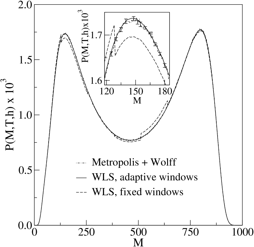
Figure 4: Magnetization probability distribution $P(M,T,h)$ for $T=0.86177$ and $h=0.005$ computed from $g(E,M)$ obtained via WLS with fixed windows using case (ii) above (dashed line), adaptive windows (solid line), and from a hybrid Monte Carlo (MC) method (dot-dashed line). In the inset only a few typical error bars are shown for the hybrid MC result (error bars for the WLS with adaptive windows are slightly smaller).

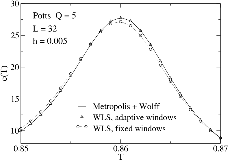
Figure 5: Specific heat versus temperature for $h=0.005$, obtained with different sampling methods. Error bars are smaller than the symbol sizes.

The discontinuities in the probability distributions, and the systematic error in thermodynamic quantities arise because the slope of the JDOS is discontinuous at the borders between neighboring fixed windows. These problems can be partly circumvented by using a larger overlap region, so that the JDOS used in the calculation of thermodynamic properties does not come from the immediate vicinity of any border. The disadvantage of such an approach is that the overlap between adjacent windows has to be quite large. There is, moreover, no guarantee that these regions will be sampled properly. Using adaptive windows, by contrast, the slopes of the JDOS at the borders of neighboring windows are equal to within numerical uncertainty. (In WLS with adaptive windows, we normalize the JDOS by applying a least-square-difference criterion along the line of overlap between neighboring sampling windows.)

The magnetization probability distribution computed from $g(E,M)$ (obtained from an average over ten independent runs using WLS with adaptive windows), is also shown in Figure 4 (solid line). This result is in good agreement with the distribution obtained using a hybrid Monte Carlo method landau_binder with $10^{8}$ MC steps. Here one MC step comprises $4L^{2}$ single spin-change trials with the Metropolis algorithm and $6$ Wolff cluster updates. (In the main graph of Fig.4 the result from adaptive-window WLS is almost indistinguishable from that using hybrid MC.) The specific heat obtained with WLS using adaptive windows is also in excellent agreement with the result of the hybrid Monte Carlo method, as shown in Fig.5. Although we illustrate the effectiveness of WLS with adaptive windows for $L=32$, a relatively small lattice size, the reader should recall that we are performing two-dimensional random walks; therefore, the parameter space is much larger than for a one-dimensional random walk using the same system size. The resulting JDOS allows us to obtain thermodynamic quantities for the entire $(T,h)$ space. We note in passing that because the 5-state Potts model has a very weak first-order phase transition, the hybrid Monte Carlo method, employed here to test our new method, can be used to sample equilibrium states; however, as $Q$ increases, it becomes forbiddingly difficult for this method to equilibrate the system using currently available computational resources. In contrast, the WLS method works well even in the presence of strong first-order phase transitions and, when combined with the adaptive windows method presented here, can be used to simulate quite large systems.

In summary, we show how WLS, arguably the most promising method presently available for simulating complex spin and fluid models, may be applied reliably to large systems without border effects. For the models considered here, such effects are strong and effectively prohibit the study of large systems using fixed windows. In our method, errors that may arise near the border of a given window are corrected in subsequent stages, in which the border positions are shifted. We expect this improvement of WLS to find broad application in studies of polymers, spin systems with complex phase diagrams, and complex fluids.

We are grateful to CAPES, CNPq, FUNAPE-UFG, Fapemig (Brazil), and NSF grant number DMR-0341874 (USA) for financial support.

References

- (1) F. Wang and D. P. Landau, Phys. Rev. Lett. 86, 2050 (2001).
- (2) F. Wang and D. P. Landau, Phys. Rev. E 64, 056101 (2001).
- (3) D. P. Landau and F. Wang, Comput. Phys. Commun. 147, 674 (2002); F. Wang and D. P. Landau, Braz. J. Phys. 34, 354 (2004).
- (4) For a partial list of applications of WLS, see e.g., D. P. Landau, S.-H. Tsai, and M. Exler, Amer. J. Phys. 72, 1294 (2004).
- (5) A. G. Cunha-Netto, C. J. Silva, A. A. Caparica and R. Dickman, Braz. J. Phys. 36, 619 (2006).
- (6) T.S. Jain and J.J. de Pablo, J. Chem. Phys. 116, 7238 (2002); J. Chem. Phys. 118, 4226 (2003).
- (7) F. Rampf, K. Binder, and W. Paul, J. Polym. Sci. Part B: Polym. Phys. 44, 2542 (2006); W. Paul, T. Strauch, F. Rampf, and K. Binder, Phys. Rev. E 75, 060801(R), (2007).
- (8) D. F. Parsons and D. R. M. Williams, Phys. Rev. E 74, 041804 (2006); J. Chem. Phys. 124, 221103 (2006).
- (9) N. Rathore and J.J. de Pablo, J. Chem. Phys. 116, 7225 (2002); J. Chem. Phys. 118, 4285 (2003).
- (10) T. Wüst and D. P. Landau, Comput. Phys. Commun. 179, 124 (2008).
- (11) C. Zhou, T. C. Schulthess, S. Torbrügge, and D. P. Landau, Phys. Rev. Lett. 96, 120201 (2006); C. J. Silva, A. A. Caparica, and J. A. Plascak, Phys. Rev. E 73, 036702 (2006).
- (12) B.J. Schulz, K. Binder, M. Müller, and D.P. Landau, Phys. Rev. E 67, 067102 (2003).
- (13) A. G. Cunha-Netto, A. A. Caparica and R. Dickman, unpublished.
- (14) S.-H. Tsai, F. Wang, and D. P. Landau, Braz. J. Phys. 38, 6 (2008).
- (15) A. Baumgärtner, J. Phys. (Paris) 43, 1407 (1982).
- (16) J. F. Douglas and T. Ishinabe, Phys. Rev. E 51, 1791 (1995).
- (17) See, e.g., D. P. Landau and K. Binder, A Guide to Monte Carlo Simulation in Statistical Physics, 2nd Edition (Cambridge University Press, Cambridge, 2005).
- (18) F. Y. Wu, Rev. Mod. Phys. 54, 235 (1982).
- (19) W. H. Press, S. A. Teukolsky, W. T. Vetterling, and B. P. Flannery, Numerical Recipes, The Art of Scientific Computing, 2nd Edition (Cambridge University Press, Cambridge, 1992).