Coupling MOAO with Integral Field Spectroscopy: specifications for the VLT and the E-ELT

Abstract

Elucidating the processes that governed the assembly and evolution of galaxies over cosmic time is one of the main objectives of all of the proposed Extremely Large Telescopes (ELT). To make a leap forward in our understanding of these processes, an ELT will want to take advantage of Multi-Objects Adaptive Optics (MOAO) systems, which can substantially improve the natural seeing over a wide field of view. We have developed an end-to-end simulation to specify the science requirements of a MOAO-fed integral field spectrograph on either an 8m or 42m telescope. Our simulations re-scales observations of local galaxies or results from numerical simulations of disk or interacting galaxies. The code is flexible in that it allows us to explore a wide range of instrumental parameters such as encircled energy (EE), pixel size, spectral resolution, etc. For the current analysis, we limit ourselves to a local disk galaxy which exhibits simple rotation and a simulation of a merger. While the number of simulations is limited, we have attempted to generalize our results by introducing the simple concepts of “PSF contrast” which is the amount of light polluting adjacent spectra which we find drives the smallest EE at a given spatial scale. The choice of the spatial sampling is driven by the “scale-coupling”. By scale-coupling we mean the relationship between the IFU pixel scale and the size of the features that need to be recovered by 3D spectroscopy in order to understand the nature of the galaxy and its substructure. Because the dynamical nature of galaxies are mostly reflected in their large-scale motions, a relatively coarse spatial resolution is enough to distinguish between a rotating disk and a major merger. Although we used a limited number of morpho-kinematic cases, our simulations suggest that, on a 42m telescope, the choice of an IFU pixel scale of 50-75 mas seems to be sufficient. Such a coarse sampling has the benefit of lowering the exposure time to reach a specific signal-to-noise as well as relaxing the performance of the MOAO system. On the other hand, recovering the full 2D-kinematics of z$\sim$4 galaxies requires high signal-to-noise and at least an EE of 34% in 150 mas (2 pixels of 75 mas). Finally, we carried out a similar study for a hypothetical galaxy/merger at z=1.6 with a MOAO-fed spectrograph for an 8m, and find that at least an EE of 30% at 0.25 arcsec spatial sampling is required to understand the nature of disks and mergers.

1 Introduction

Developing a coherent model for the mass assembly of galaxies over cosmic time is a complex and difficult task. It is difficult because developing such a coherent model involves highly non-linear physics (e.g., the cooling and collapse of baryons, or feedback from stars and super-massive blackholes which regulate both the growth of the stellar mass and black holes themselves) and all over a very wide range of physical scales (from large scale structure to star clusters to black holes). Our knowledge of galaxy formation in situ relies mostly on observations of integrated quantities,which is insufficient to understand the details of the process of formation, e.g., the interplay between the baryonic and dark matter, or the complex physics of baryons such as merging, star formation, feedback, various instabilities and heating/cooling mechanisms, etc. At the heart of our developing understanding of galaxy evolution is the relative importance of secular evolution through (quasi-)adiabatic accretion of mass, instabilities, and resonances (e.g., Semelin & Combes 2005), versus more violent evolution through merging (e.g., Hammer et al. 2005), as a function of look-back time.

Because of the complexity of the processes involved, understanding the mass assembly of galaxies over cosmic time requires constraining a wide range of phenomenology for large samples of objects. In this respect integral field spectroscopy is particularly well suited in that it allows us to map the spatially resolved physical properties of galaxies (see, e.g., Puech et al. 2006b). Unfortunately, splitting the light into many channels in a integral field spectrograph requires long integration times, even on large telescopes, to detect low surface brightness emission. Thus, conducting large statistical studies necessary for understanding the processes driving galaxy evolution will demand a high multiplex capability to efficiently investigate sufficient numbers of objects.

Using current facilities on 8m class telescopes, it is already possible to map the physical properties of distant galaxies. For example, FLAMES/GIRAFFE on the VLT offers the unique ability to observe 15 distant galaxies simultaneously. The first (complete) 3D sample of galaxies at moderate redshifts has revealed a large fraction ($\sim$40%) of all z$\sim$0.6 galaxies with $M_{B}<$-19.5 have perturbed or complex kinematics (Flores et al. 2006; Yang et al. 2008). This population of dynamically disturbed galaxies is most probably a result of a high prevalence of mergers and merger remnants (see also Puech et al. 2006a, 2008). At higher redshift, integral field spectroscopy of several objects has been obtained using single object integral field spectrographs available on 8-10 meter class telescopes (e.g., Förster-Schreiber et al. 2006). However, many of these data sets were obtained with limited spatial resolution sampling galaxies on scales of a few kpc, and the true dynamical nature of many sources sampled at these spatial and spectral resolutions remains uncertain (e.g., Law et al. 2007).

Improving and extending this approach to the general understanding of the nature of faint galaxies and to galaxies in the early Universe will require a new generation of multi-object integral field spectrographs working in the near-IR, with increased sensitivity and better spatial resolution on even larger telescopes. Because of the complex interplay between spatial and spectral features and our limited knowledge of high redshift galaxies, it is helpful, perhaps necessary, to rely on numerical simulations for constraining the design parameters of this new kind of instrument. For this purpose, we have developed software that simulate end-to-end the emission line characteristics of local galaxies and numerical simulations of galaxies to show how they would appear in the distant Universe. By changing various parameters like the resolution, pixel scale, and point spread function it is possible to constrain the instrumental characteristics and performance against a set of galaxy characteristics (e.g., velocity field). This paper is the first in a series to investigate the scientific design requirements of possible future instruments, telescope aperture and design, and site characteristics appropriate for constrain how galaxies grew and evolved with cosmic time. In this paper in particular, we aim to present the details of our assumptions that go into the software, as well as a first attempt to constrain some of the high level specification for a hypothetical but realistic multi-object integral field spectrograph assisted by MOAO system. Because 2D kinematics (i.e., velocity field and velocity dispersion maps) are one of the most obvious and easiest to currently simulate, they provide the most straight forward way of constraining the high level science design requirements for this type of instrument. We emphasize that the goal of this paper is not to study the detailed scientific capability of such instruments. Instead, the present paper aims at examining a few scientifically motivated cases to derive relevant specifications for such types of instruments with a capable MOAO system. These specifications will then be adopted as a baseline for studying their scientific capabilities subsequent papers. This paper is organized as follows: in Section 2, we detail the goals of this study and our methodology; in Sect. 3 we present the new simulation pipeline and in Sect. 4 how MOAO PSFs are simulated; In Sect. 5 we describe the kinematic measurements; In Sect. 6 and 7, we present the simulations and their results, which are discussed in Sect. 8. In Sect. 9, we draw the conclusions of this study.

2 Specifying MOAO-fed spectrographs

2.1 MOAO & 3D spectroscopy: EAGLE and FALCON

Most of current dynamical studies of distant galaxies are severely hampered by their limited spatial resolution, which introduces an important uncertainty as to their dynamical nature as discussed in the Introduction. A MOAO-fed integral field spectrograph on the VLT and/or the E-ELT will improve substantially the spatial resolution compared to non-AO assisted observations. The concept of MOAO was first proposed in the FALCON design study, a multi objects 3D spectrograph intended for the VLT (Hammer et al. 2002). Briefly, the main objectives of the FALCON concept was to obtain 3D spectroscopy of distant emission line galaxies, up to $z\sim 2$. Doing this requires us to observe in the near infrared since all of the important optical emission lines from [OII]$\lambda$3727Å  to H$\alpha$ are redshifted into the atmospheric windows from 0.8 to 2.5 $\mu$m (see, e.g., Hammer et al. 2004). Because the intrinsic size of distant galaxies is small, AO is needed to spatially resolve emission lines and thus to keep the spectroscopic signal-to-noise ratio (SNR) high enough to detect small features. Correcting a large field of view (FoV) to observe many galaxies simultaneously is challenging and normal single natural guide star AO is not sufficient. MOAO is a method for obtaining excellent correction over a relatively large FoV ($\geq$few arcmin). The basis of this concept is to correct only regions where the targets lie, instead of correcting the entire FoV of the instrument. MOAO uses atmospheric tomography techniques (Tallon & Foy 1990; Tokovinin et al. 2001) meaning several wave-front sensors (WFS) for each integral field unit (IFU) measure the off-axis wavefront coming from stars located within the FoV, and the on-axis wavefront from the galaxy is deduced from off-axis measurements and corrected by an AO system within the optical train of each IFU. A detailed description of FALCON can be found in Assémat et al. (2007). The general concept of MOAO was subsequently adapted to the future European Extremely Large Telescope (E-ELT) in the WFSPEC study (Moretto et al. 2006), which was a precursor to the current EAGLE concept. One of the most important goals in setting the science design requirements for EAGLE is mapping the physical properties of galaxies up to z$\sim$5, in order to better understand the processes that drive the evolution of galaxies.

2.2 Goals of this study

As a first study, we want to help derive high-level design specifications for the EAGLE and FALCON MOAO-fed instruments by addressing the following:

• Explore the necessary order of magnitude of integration times that will be required to reliably derive the kinematics of distant emission line galaxies, allowing their classification;

• By selecting a simple rotating disk with little substructure and a merger simulation with two overlapping disks, explore the most relaxed requirements for the design of the instrument in terms of the necessary adaptive optics performance and coarseness of the pixel scale. To this end we have limited our simulations to spatial sampling of 50-75 mas pixel^-1;

• Help constrain the requirements on the MOAO system by specifying its spectroscopic coupling (which is defined here as the Ensquared Energy [EE] per element of the spatial resolution, see Sect. 4).

A detailed study of the scientific capabilities of these instruments is beyond the scope of this paper. Instead, we want to use a limited number of comparisons between scientifically motivated cases in order to help derive the most relaxed high-level specifications.

2.3 Methodology

Flux is the zero-order moment of an emission line, while the velocity and width are the first and second moment, and higher order moments always have more relative uncertainty. For this reason, kinematics will set stringent requirements on the SNR necessary to fully characterize faint extended emission line gas.

The characteristics of these moments depend on the underlying source of an emission line’s excitation and kinematics. Because the most easily reached goal of MOAO-fed spectrographs will be to understand the kinematics of the emission line gas in galaxies, a natural kinematic reference case for such a study is a simple spiral rotating disk. In the following we will use Fabry-Perot observations of the local rotating disk UGC5253 taken as part of the GHASP survey (Amram et al. 2002; see its main photometric and dynamical properties in Tab. 1; see also Fig. 1) as such a reference case.

UGC	Type	z	D(’)	MB	inc($\deg$)	Vmax
5253	SA(rs)ab	0.004306	4.168	-20.8	40	261.8

Table 1: Main photometric and dynamical properties of UGC5253, used as a typical rotating disk in the simulations: Morphological type (from Garrido et al. 2002), redshift (from CDS), absolute B-band magnitude, inclination, and maximal velocity of rotation (from Garrido et al. 2002).

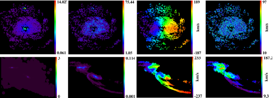
Figure 1: Morphology and kinematics of the two objects used in the simulations. Up: UGC5253 (rotating disk). Down: Merging between two Sbc galaxies. From left to right: continuum map, monochromatic map, velocity field, and velocity dispersion map. The original spatial scale is $\sim$85 pc/pix for UGC5253, and $\sim$200 pc/pix for the merger simulation. These templates are rescaled in terms of size and flux to simulate realistic distant galaxies.

Several different mechanisms have been proposed to explain how galaxies assembled their mass: major mergers (merging between galaxies having similar masses), minor mergers (merging between galaxies with a mass ratio larger than 5:1), and gas accretion (of cold or hot gas from the IGM or dark matter halo). For each of these processes, there are a large number of possible configurations or characteristics that need to be modeled or analyzed (e.g., mass ratio of merging galaxies, the relative angular momentum vectors of each merging galaxy and of the orbit, the temperature and density distribution of the gas as it is being accreted, etc.). However, our goal here is not to conduct a systematic study of the scientific capabilities of MOAO-fed spectrograph in discriminating between all possible evolutionary mechanisms. Instead, we want to investigate the surface brightness limits of such instruments and focus on the possibility to use a relatively coarse spatial resolution to recover large scale motions, whereby the process underlying the dynamics may be divined (following for example Flores et al. 2006; Puech et al. 2006a; Yang et al. 2008). Because we only want to help determine plausible design requirements relative to this goal, it is sufficient to explore the most extreme large-scale kinematic patterns, which are produced by major mergers. Indeed, during such processes, the disks of the progenitors are usually completely destroyed, which leads to complex kinematic patterns with abrupt changes in the velocity gradient(s). In the following, we will use a major merger extracted from an hydrodynamic simulation of a pair of two merging Sbc galaxies (Cox et al. 2006), just before the bodies of the two galaxies coalesce, but are still discrete entities, which also provides us with the relaxed requirements in terms of spatial resolution (see Fig. 1). In addition, the relatively low surface brightness extended gas produced during such events (see, e.g., the tidal tail in Fig. 1) will also allow us to explore the ability of MOAO in recovering such faint discrete features. Trying to detect these features again emphasizes our choice of simulations and is really leading toward constraints that optimize for surface brightness detection and away from resolving structures within disks and in the chaotic central regions of advanced mergers. In the next three sections, we describe the different steps of this study: (a) Simulation of data-cubes (Sect. 3); (b) Simulations of MOAO PSFs (Sect. 4); (c) Kinematic analysis of the data-cubes (Sect. 5).

3 An end-to-end simulation pipeline for 3D spectroscopy

3.1 General Description

The main steps of the process can be summarized as follows. First, a data-cube with with the spatial resolution of the telescope diffraction limit (i.e., $\sim\lambda/2D$, where D is the telescope diameter) is generated. For each pixel of this high resolution data-cube, a spectrum is constructed from observations of local galaxies or results from numerical simulations. In the second step the spatial resolution of the data-cube is reduced by convolving each spectral and spatial pixel of the high resolution data-cube by a PSF. This PSF used in this convolution is representative of the optical path through the atmosphere and the telescope up to the output of the (optional) AO system. In the third step, the spatial sampling of the data-cube is reduced to match that of the IFU of the simulated instrument. Finally, realistic sky as well as photon and detector noise are added. Note that this software can also be used to simulate images of distant galaxies, since an image can be viewed as a particular case of a data-cube, with a single broad-band spectral channel. We now describe each step in detail; all input parameters are summarized in Table 2.

3.2 High resolution data-cube

At very high spatial resolution, emission lines with kinematics driven only by gravitational motions is well described by a simple Gaussian (Beauvais & Bothun 1999). Under this assumption, for each pixel of the data-cube, only four parameters are required to fully define a spectral line. The first three parameters are the position in wavelength, the width, and the area (or, equivalently the height) of the emission line. The current version of the software only models emission lines and does not take into account the detailed shape of the continuum in galaxies – it is simply modeled as a constant in f_λ. So only one parameter is required to set the level of this pseudo-continuum around the emission line. We assumed a perfect Atmospheric Dispersion Corrector (ADC) and did not take into account atmospheric refraction effects (see, e.g., Goncharov et al. 2007). Each spectrum is generated in the observational frame, at a given spectral sampling of $\lambda_{obs}$/$2R$, where $R$ is the spectroscopic power of resolution of the instrument, and $\lambda_{obs}\sim(1+z)\lambda_{em}$, $\lambda_{em}$ being the rest-frame wavelength of the emission line, and $z$ the redshift of the simulated object. During this process, the rest-frame line width is multiplied by (1+z), as one needs to take into account the widening of emission lines with increasing redshift.

All four parameters can be extracted from observations of local galaxies. In the following, we use Fabry-Perot (FP) observations of the H$\alpha$ emission distributions of nearby galaxies obtained as part of the GHASP survey (Amram et al. 2002). From these data, we can extract four parameters, wavelength, width, area, and continuum level to construct the velocity field, the velocity dispersion map, the flux map of the H$\alpha$ emitting gas, and the continuum map of the galaxy. The software first re-scales all these maps at a given angular size (in arcsec) provided by the user. These maps are then interpolated at a spatial sampling of $\sim\lambda/2D$. This spatial sampling is motivated by the fact that the AO PSFs used have been simulated at this sampling (see §4). The software then re-scales the overall amplitude of the continuum map at a given integrated number of photons using an integrated magnitude $m_{AB}$ directly provided by the user. This magnitude is converted to the number of photons per spectral pixel depending on the telescope diameter $D$, the integration time $t_{intg}$, and the global transmission $t_{trans}$ of the system (atmosphere excluded). The overall amplitude of the H$\alpha$ map is also rescaled with a given integrated number of photons, derived from the integrated continuum value and a rest-frame equivalent width $EW_{0}$ provided by the user, the latter being re-scaled in the observed-frame by multiplying by (1+z).

All parameters can also be extracted from outputs of hydro-dynamical simulations (Cox et al. 2004). In this case, the last two parameters (area and continuum level) can respectively be extracted from total gas and stellar surface density maps which are by-products of the numerical simulation, also rescaled in terms of size and flux.

3.3 Modeling the IFU and the detector

Each monochromatic slice of the high resolution data-cube is convolved by a PSF with matching spatial sampling. This PSF must be representative of all elements along the optical path, from the atmosphere to the output of an (optional) Adaptive Optic system. Because the isoplanetic patch (Fried 1981; the median value at Paranal is $\sim$2.4 arcsec at $\lambda\sim$ 0.5 $\mu$m, which leads, e.g., to $\sim$10 arcsec at $\lambda\sim$ 1.6 $\mu$m) is larger than the individual FoV of the IFU (typically a few arcsec, depending on the size of objects at a given redshift), the same PSF can be used to convolve the data-cube regardless of position within the IFU. We also neglected the variation of the PSF with the wavelength (with a FWHM varying as $\lambda^{-1/5}$ in a Kolmogorov model of the atmospheric turbulence, see, e.g., Roddier 1981), as we are only interested in the narrow spectral range around a single emission line.

The next step is to reduce the spatial sampling of the data-cube. This is done by re-binning each monochromatic channel of the data-cube at the pixel size $\Delta_{pix}$ of the simulated IFU. A wavelength dependent atmospheric absorption curve taken from ESO Paranal is then applied to each spectrum of the data-cube. Sky continuum, detector dark level and bias are then added to the spectra. We used a sky spectrum model (including zodiacal emission, thermal emission from the atmosphere, and an average amount of moonlight) from Mauna Kea, which has the advantage over other available sky spectra to be very well sampled with 0.2 Å/pixel. Photon and detector noise are then added to each individual exposure. The detector noise is due, in the NIR, to the dark current ($dark$), and readout noise ($ron$). The simulation pipeline generates $ndit$ data-cubes with individual exposure time of $dit$, which are combined by estimating the median of each pixel to simulate several individual realistic exposures. Since we have only included random noise, it is similar to having dithered all of individual exposures and combining them after aligning them spatially and spectrally. The spectroscopic SNR is then derived as follows:

$$SNR(i_{x},j_{y},k_{\lambda})=\frac{O(i_{x},j_{y},k_{\lambda})*\sqrt{ndit}}{\sqrt{O(i_{x},j_{y},k_{\lambda})+S(i_{x},j_{y},k_{\lambda})+ron^{2}+dark}},$$

where $O(i_{x},j_{y},k_{\lambda})$ and $S(i_{x},j_{y},\lambda)$ are respectively the object and sky flux per $dit$ (after accounting for atmospheric transmission) in the spatial position $(i_{x},j_{y})$ of the data-cube (in pixels), and at the spectral position $k_{\lambda}$ along the wavelength axis (in pixels). In the following, the “maximal SNR in the emission line in the pixel $(i_{x},j_{y})$” refers to MAX${}_{k_{\lambda}}$[$SNR(i_{x},j_{y},k_{\lambda})$], and the “total SNR” refers to the flux weighted average of this quantity over the galaxy (i.e., the spatially integrated SNR in the spectral pixel where the emission line peaks, and not the spatially integrated SNR within the whole emission line width, as sometimes used in other studies).

Parameter	Description (Unit)	EAGLE/E-ELT	FALCON/VLT
$M1$	Telescope Primary mirror size (m)	42	8.2
$M2$	Telescope Secondary mirror size (m)	0	1.116
$R$	Spectral resolution power	5000	5000
$\Delta_{pix}$	IFU pixel size (arcsec)	0.075”	0.125”
$t_{transm}$	Telescope + Instrument transmission factor	0.2	0.2
$dark$	Dark level (e/sec/pix)	0.01	0.01
$ron$	Read-out-noise (e/pix)	2.3	2.3
$dit$	detector integration time (s)	3600	3600
$ndit$	Number of dit per simulation	200-24-8	200-24-8
$z$	Redshift of the object	4.0	1.6
$S$	Object angular diameter (arcsec)	0.8	2.0
$m_{AB}$	Integrated magnitude of the object continuum (AB mag)	24.5	22.5
$\lambda_{em}$	Emission line wavelength (Å)	3727	6563
$EW_{0}$	Equivalent width at rest of the emission line (Å)	30	50

Table 2: First and second columns: Input parameters of the simulation pipeline provided by the user. Third column: parameters used for the simulations of z=4 galaxies with EAGLE on the E-ELT. Fourth column: parameters used for the simulations of z=1.6 galaxies with FALCON on the VLT.

4 Generating MOAO PSFs

The coupling between the MOAO system and the 3D spectrograph is captured through the MOAO system PSF. Therefore, it is a crucial element that needs to be carefully simulated, and cannot be approximated by, e.g., a simple Gaussian. We describe here how these PSFs were modelled, and briefly describe how the MOAO correction influences the PSF shape at the spatial scale of the instrument IFU.

4.1 MOAO PSFs for EAGLE

A preliminary study of the PSF shape generated by a hypothetical MOAO system can be found in Neichel et al. (2006). In the following, we used eight PSFs generated in a similar manner as in the Neichel et al. study. Briefly, three off axis guide stars, located at the edges of an equilateral triangle, are used to perform a tomographic measurement of the turbulent atmospheric volume. We have used a turbulent profile typical of that on Cerro Paranal, which can be modeled using three equivalent layers (Fusco et al. 1999). The seeing and the outer scale of the turbulence were respectively set to 0.95 arcsec (at 0.5 $\mu m$, the $\sim$0.75 percentile on Paranal) and to 22m (the median value on Paranal). Guide stars are assumed to be bright (V$\sim$13), i.e., WFS noise is neglected. The optimal correction is deduced from the characteristics of the turbulence volume and applied assuming a single Deformable Mirror (DM) per direction of interest, here taken as the center of the guide star constellation. To explore a wide range of correction, we consider different GS-constellation sizes, as well as a DM with an inter-actuator size of either 1 m or 0.75 m in the pupil plane (for a 42 meter telescope), which corresponds to 42x42 or 56x56 actuators (see Tab. 3). Of note, the SPHERE eXtreme AO (XAO) project (Beuzit et al. 2006) will use a 41x41 actuators DM (Fusco et al. 2006). PSFs are shown in Figure 2.

Pitch	FoVWFS	EE	Strehl Ratio (%)
1.00	4.00	22	0.1
1.00	3.00	24	0.2
1.00	2.00	26	0.6
1.00	1.00	31	3.9
1.00	0.50	34	6.7
1.00	0.25	40	11.5
1.00	0.00	43	10.5
0.75	0.00	47	11.7

Table 3: AO system parameters used for the simulation of the EAGLE PSFs. The EE is given in 0.15 arcsec, and the pitch corresponds to the inter-actuator distance on the telescope pupil, in meters. The second column gives the diameter of the constellation of three stars (at equal distance of the central galaxy) used to sense the wavefront, in arcmin. Strehl Ratios are given in the last column.

Usually, AO PSFs are characterized using the Strehl Ratio [SR], which provides a useful way for comparing different PSFs relatively to the diffraction limited case. However, MOAO does not provide diffraction limited PSFs but performs only partial corrections in order to increase the spectroscopic coupling with the 3D spectrograph (Assémat et al. 2007), which cannot be easily described by using the SR. Instead, the spectroscopic coupling can be directly quantified by the fraction of light under the PSF that enters a spatial element of resolution of the IFU, i.e., the Ensquared Energy entering an aperture equal to twice the IFU pixel size. Such a parameter is an extrapolation of the classical “Encircled Energy” used in optics to characterize optical system quality, and is directly related to the achieved SNR. It is therefore a more natural choice to parametrize the MOAO performance than the SR. In the presence of speckle noise on the PSF as it is the case in the end-to-end MOAO simulations used here, the SR measurement can be severally affected by this noise, which produces artificially low SR values and contributes to disconnect the SR measurement from the spectroscopic coupling: at a given EE, a PSF affected by speckle noise will have a lower SR than a PSF without speckle noise, all else being equal. We list both SR and EE for the simulated PSFs in Tab. 3.

To explore how the AO correction impacts the PSF shape, we first derived the PSF FWHM using Sextractor (Bertin & Arnouts 1996). We compared these to their Ensquared Energy [EE] in a aperture equal to twice the pixel size (i.e., 0.15 arcsec) in Fig. 3. The EE is measured as the fraction of light under the PSF that enters this aperture. Fig. 3 reveals two regimes, depending on the EE. In the first regime, the EE and the FWHM are roughly linearly correlated, so that the EE can alternatively be used as an indirect measure of the FWHM. This regime corresponds to the formation of a central diffraction limited core in the PSF. When the adaptive system does not correct for the overall atmospheric turbulence, it is indeed well known that the resulting PSF can be approximately described by a double core-halo structure, with a coherent central diffraction-limited peak surrounded by seeing-limited wings. This regime corresponds to an improvement of the spatial resolution, as long as the PSF FWHM remains larger than twice the IFU pixel scale. When the PSF FWHM becomes smaller than twice the IFU pixel size, the spatial resolution is now set up by the IFU pixel scale. In this case, the AO corrections does not dramatically influence the spatial resolution any longer, but can still provide better EE and SR by further narrowing the core below the IFU pixel scale (see Tab. 3), which translates into an improvement of the SNR. When EE$\geq$27-30%, the diffraction limited core is now well formed, which explains why the measurement of the FWHM of the PSF saturates, since the FWHM is then only sensitive to the PSF central core as it does not “see” the residual halo around it. In this new regime, the SR keeps rising with the EE because the AO system is still able to bring energy located in the PSF halo into the central diffraction limited peak. In most situations, the MOAO system will provide EE larger than this limit, which justifies the choice of characterizing the EE in an aperture equal to twice the pixel size.

In the intermediate regime where the PSF FWHM is smaller than twice the IFU pixel scale, but where the diffraction core is not completely formed (e.g., EE ranging between 23 and 35% in Fig. 3), the PSF halo can be an important limitation in the observations of high redshift galaxies, because it can result in a mixing of the spectra coming from adjacent spatial elements of resolution. In the following, we use the total energy entering the first ring of 0.15 arcsec apertures around the one centered on the PSF to measure this effect. This provides a useful proxy to quantify the amount of light coming from adjacent spatial element of resolution, and polluting the element of resolution centered on the PSF. We called this effect “PSF cross-talk” (PCT), by analogy with the instrumental crosstalk, which measures the amount of scattering that spreads information beyond the PSF due to instrumental effects. Figure 3 also compares the PCT with the EE for the set of eight simulated PSFs, and shows a linear correlation between these two parameters: while the AO system provides a better correction, the energy located in the wings of the PSF is brought into the central diffraction-limited core (see Assémat et al. 2007), increasing the EE and decreasing the PCT. PCT gives as useful measurement of the “PSF contrast”: having a PCT smaller than 50% means that the light entering a spatial element of resolution is not dominated by polluting light coming from adjacent spatial elements of resolution. In the EAGLE case and at a pixel scale of 75 mas, this occurs at EE$\sim$35% (see Fig. 3).

Figure 2: Transverse cut of the simulated EAGLE MOAO PSFs. The EE in 0.15 arcsec increases from bottom to top: 22%, 24%, 26%, 31%, 34%, 40%, 43%, and 47%. The vertical dashed-lines represent the spatial element of resolution used for EAGLE simulations, i.e., 0.15 arcsec.

Figure 3: Top: FWHM vs. EE (in 0.15 arcsec) for the eight simulated EAGLE PSFs. The dotted line represents the diffraction limit on a 42m ELT in H band, i.e., $\lambda_{diff}(H)=0.008$ arcsec. The black line is an exponential fit between the FWHM and the EE, and the dotted-dashed line is a simple linear fit to the three first points. The dashed lines shows when the FWHM becomes lower than 0.15 arcsec, i.e., twice the pixel size (under-sampling of the PSF). Bottom: PCT vs. EE for the eight simulated EAGLE PSFs. The black line is a simple linear fit between PCT et EE.

4.2 MOAO for FALCON

An extensive study of the FALCON MOAO system has been carried out by Assémat et al. (2007). As part of this study, a simulation pipeline of FALCON PSF was developed. We used this tool to generate a set of eight PSFs (see Fig. 4). All PSFs were simulated using typical atmospheric conditions at ESO/Paranal. Briefly, a median seeing of 0.81 was used, with an outer scale of the turbulence of 24m, and an atmosphere model composed of three layers located at [0,1,10]km with respective weights of [20, 60, 20]%. We set the parameters of the MOAO system in order to explore a wide range of EE in 0.25 arcsec (twice the pixel size), ranging from 19% to 46% (see Tab. 4). Technical details about the concept can be found in, e.g., Puech et al. (2005).

Table 4: AO system parameters used for the simulation of the FALCON PSFs. The EE is given in 0.25 arcsec, and the value quantifying the correction corresponds to the radial number n of Zernike modes corrected. The third column gives the diameter of the constellation of three stars (at equal distance of the central galaxy) used to sense the wavefront, in arcsec. Following Puech et al. (2005), n=7 corresponds roughly to a $\sim$1.4m pitch, and n=9 to a $\sim$1.1m pitch. The first PSF is the seeing limited case, with no correction. Strehl Ratio are given in the last column.

Correction	FoVWFS	EE	Strehl Ratio (%)
0	N.A.	19	1.03
7	300	26	1.56
7	180	27	1.51
7	60	31	2.26
7	30	34	4.04
7	10	35	4.55
7	60	39	20.82
9	60	46	30.03

Figure 4: Transverse cut of the FALCON MOAO PSFs simulated. The EE in 0.25 arcsec increases from bottom to top: 19%, 26%, 27%, 31%, 34%, 34%, 35%, 39%, and 46%. The vertical dashed-lines represent the spatial element of resolution used for FALCON simulations (0.25 arcsec aperture) within which EE are derived.

For this set of PSFs, we compared their FWHM and PCT to their EE in 0.25 arcsec in Figure 5, which reveals a similar behavior compared to Fig. 3. Note that when EE$\geq$30%, the FWHM becomes lower than 0.25 arcsec (i.e., twice the pixel size). This means that when EE$\geq$30%, the spatial resolution is oversampled at twice the IFU pixel size. This is why, in the following, all EE are computed in a 0.25 arcsec size aperture. Finally, PCT becomes smaller than 50% for EE$\sim$35%, which is the limit for a good “PSF contrast” in the FALCON case, at a pixel scale of 0.25 arcsec.

Figure 5: Top: FWHM vs. EE for the eight simulated FALCON PSFs. The left most point corresponds to the seeing limited PSF. The horizontal line represents the diffraction limit on the VLT in H band, i.e., $\lambda_{diff}(H)=0.04$ arcsec. The dashed lines show when the spatial resolution, as measured by the FWHM, is lower than 0.25 arcsec, i.e., twice the pixel size. The black line is a linear fit between FWHM and EE (the last point, where the FWHM saturates, has been discarded from the fit). Bottom: PCT vs. EE for the eight simulated FALCON PSFs. The left most point corresponds to the seeing limited PSF. The black line is a linear fit between the PCT and the EE.

5 Simulating and measuring 2D kinematics

5.1 Kinematic measurements

The simulated data-cubes are analyzed using a data analysis pipeline similar to those generally used to analyze data of high redshift galaxies. During this process, each spatial pixel of the simulated data-cube is fitted with a Gaussian in wavelength, whose position and width correspond to the velocity and velocity dispersion of the gas in this spatial pixel. Because the accuracy of these measurements is driven by the flux within the emission line relative to the noise in the continuum, one has to define a kinematic signal-to-noise ratio $SNR_{kin}$ specific for this measurement. We chose to rely on the definition of Flores et al. (2006), who defined $SNR_{kin}$ as the total flux in the emission line divided by the noise on the continuum $\sigma_{continuum}$ and $\sqrt{N}_{pix}$, the number of pixels within the emission line. We emphasize that this $SNR_{kin}$ is different from the classical $SNR$, as defined in Sect. 3.3: the latter quantifies the signal to noise ratio relative to the sky and detector noise (detectability of the emission line), while the former characterizes the capability of measuring the first and second order moments of the emission line, relative to the noise in the continuum (Sarzi et al. 2006). Although they are different in nature, we find that both SNRs roughly correlates provided that $SNR>3$ (corresponding the $SNR_{kin}\sim$3-4). Because a lot of data-cubes are simulated and need to be analyzed, one has to rely on a fully automatic analysis pipeline. Tests show that pixels with a “kinematic” $SNR_{kin}<$ 3 have very large errors mostly due to misidentification of emission lines with noise peaks. Hence, only pixels having a $SNR_{kin}$ of at least three have been kept for further analysis.

5.2 Kinematic diagnostic diagrams

To help distinguish between the two kinematic templates (i.e., the major merger and the rotating disk), we fitted a rotating disk model to each velocity field. This model assumes a constant dynamical center, PA, inclination, and $V_{sys}$ over the galaxy, and a simple arctan shape for the rotation curve. During the fit, the pixels of the velocity field are weighted by the corresponding error in bins of SNR, which were determined using Monte-Carlo simulations. Finally, the residuals between the velocity field and the fitted model are derived, together with the reduced $\chi^{2}$ map.

We then adopted two criteria for judging whether or not the fit to a particular simulated galaxy is appropriate. Because we are interested only in large-scale motions (i.e., circular rotation vs. non-structured motions), we need to adopt a criterion not affected by smaller-scale variations due to non-circular perturbations like, e.g., spiral arms or bars. For characterizing the 2D-fit as a whole, we therefore rely on the median $\chi^{2}_{m}(VF)$ over the galaxy. When smaller than unity, it means than at least 50% of the pixels on the velocity field are reliably fitted by a rotating disk model, and that galaxy motions are actually dominated by circular rotation. In addition, we choose to compare the distance between the fitted dynamical center and the velocity dispersion barycenter. We used such a criterion because in the case of data which are heavily smoothed by the seeing, a process that leads to more complex dynamics like merging would only rarely have its dynamical center of the entire system coincident with the maximum in the distribution of velocity dispersions. For this, we derived the associated uncertainty, using classical propagation of errors due to the uncertainties on the dynamical center fit and on the sigma barycenter. We then derived a parameter $\Delta\sigma_{peaks}$ defined as the distance between the fitted dynamical center and the velocity dispersion barycenter, normalized by the corresponding uncertainty. Having $\Delta\sigma_{peaks}<1$ means that the fitted dynamical center is found close enough to the sigma barycenter location relative to the associated uncertainty, to be considered as compatible with the dynamics of a rotating disk.

In summary, the kinematics of a galaxy can be considered as compatible with that of a rotating disk, provided that it falls on a region of a “diagnostic diagram” ($\chi^{2}_{m}(VF)$,$\Delta\sigma_{peaks}$) where the median normalized residual is smaller than one, and provided that $\Delta\sigma_{peaks}\leq$ 1. We need to emphasize that this classification (as any) is not without limitations. As an example, let us consider a merging pair of galaxies. If both progenitors are equally distant from the center of mass of the system, the velocity dispersion map will show two peaks equally distant from this center, and the resulting barycenter of the sigma map may then be found very close to the dynamical center of orbital motions between the two progenitors if the separation of the two is small compared to the intrinsic resolution of the data and the exact distribution of the emission line gas. Of course, that is a limitation of most techniques as it can be difficult to identify close merging pairs at high redshift. It is important to be aware that there are some configurations that are difficult to distinguish between. Be that as it may, we use this approach as a first attempt in quantifying the rotation in very distant galaxies.

6 Simulations

6.1 Assumptions

It was decided not to simulate observations in the K-band as the detectability of lines in the thermal infrared is highly dependent on the achieved emissivity of the instrument. To generalize these first simulations and to remove additional free parameters, such as the telescope and instrumental emissivities and temperatures, we consider the H band only, assuming no thermal emission from the instrument and the telescope in the H-band. Our tests show that this assumption leads to overestimate the SNR in the H-band by no more than $\sim$10%. This makes these first simulations less dependent of the telescope design (e.g., number of mirrors), environmental conditions (site selection), and instrument characteristics (e.g., number of warm mirrors). Moreover, working in the H-band will help disentangle spatial effects from flux limitation arising from the high thermal background in the K-band.

For this study, we assumed a spectral power of resolution $R$=5000 as a compromise between our desire to minimize the impact of the OH sky lines and not wanting to over-resolve the line by a large factor. Moreover, appropriate targets in the NIR are usually selected as they have emission lines that fall in regions free of strong OH lines. We estimated that about one third of the H-band is free from strong sky background variations (i.e., larger that 10% of the sky continuum) in continuous windows of at least 200 km/s. Therefore, for simplicity, all simulations have been performed without OH sky lines, accounting for the sky continuum only. Usually, R=3000 is considered as a strict minimal spectral resolution to work between OH sky lines. In comparison, R=5000 will allow a better sky subtraction and limit kinematic measurement (i.e., velocity and velocity dispersion) uncertainties. In addition, for simplicity, we assume that the [OII] emission line is a single line, instead of a doublet. This does not influence any results presented here, as these are scaled with the total flux, i.e. the flux inside both lines of the doublet (assuming the low density limit for the ratio of the two lines).

The instrumental parameters of the simulation were set to typical values used in the IR (see Tab.2), relying on a cooled Rockwell HAWAII-2RG IR array working at $\sim$80K, as described by Finger et al. (2006). An array of this type is already used in SINFONI, and arrays with similar characteristics will be implemented in next VLT generation IR instruments such as HAWK-I, KMOS, or X-SHOOTER. Table 2 summarizes the main parameters used in the simulations.

Previous studies of FALCON have considered a pixel scale of 0.125 arcsec (Puech & Sayède 2004; Assémat et al. 2007). We will thus adopt this scale in the following. For EAGLE, we chose to firstly explore a pixel scale of 75 mas. This choice is suggested by recent 2D-kinematical studies of distant galaxies with GIRAFFE, which show that a relatively coarse pixel scale can already provide us with enough information to properly recover large scale motions in distant galaxies, and then discriminate between simple rotating disks and major mergers (see Flores et al. 2006; Puech et al. 2006a).

6.2 Simulation of z$\sim$4 galaxies with EAGLE

We conducted simulations at z=4, where the [OII] emission line falls in the H band. Both objects have been rescaled in half-light radius and flux to account for evolution and redshift (see bottom of Tab.2). Ferguson et al. (2004) and Bouwens et al. (2004) found that the typical r_half of z$\sim$4 galaxies is $\sim$0.2 arcsec in the UV. Hence, we adopted an optical diameter of 0.8 arcsec for z$\sim$4 galaxies ($R_{opt}\sim 2r_{half}$). The continuum magnitude was chosen considering Yoshida et al. (2006), who studied z$\sim$4 Lyman Break Galaxies luminosity functions in the UV. They found a typical UV magnitude of 24.5. We neglected any color corrections between UV and blue optical ([OII]$\lambda$3727Å): as spiral Spectral Energy Distributions [SEDs] rise from UV to optical, this choice can be considered as a minimal value for a typical pseudo-continuum for z$\sim$4 galaxies. We assumed an integrated rest-frame equivalent-width EW₀([OII])=30Å, extrapolating the median values found in z$<$1 galaxies by Hammer et al. (1997). This leads to an integrated emission line flux $\sim$7.5$\times$10^-18erg/s/cm² (observed-frame).

6.3 Simulations of z$\sim$1.6 galaxies with FALCON

We choose as a rest-frame Equivalent Width $EW_{0}$ for the H$\alpha$ emission line, the minimal value observed in the sample of Erb et al. (2006) at z$\sim$2. In their sample, the continuum at 1500Å  ranges from $m_{AB}$ = 22 to 26. Assuming a U-H color of 3.5, typical of Sa-Sb galaxies (Mannucci et al. 2001), and assuming that this value can be extrapolated at z$\sim$1.6, this leads us to a minimal magnitude in the H band of $\sim$22.5. As a cross-check, we looked at the sample of BM/BX galaxies of Reddy et al. (2006). We found 22 sources having a redshift between 1.4 and 1.8, for which Reddy et al. give J and K bands AB magnitudes. Assuming that the H-band magnitude can roughly be approximated by an average between J and K bands magnitudes, we found in these 22 sources, a median (mean) H-band magnitude of 22.55 (22.56). We can thus assume with some confidence that m_AB(H)=22.5 is quite representative of luminous z$\sim$1.6 galaxies. This leads to an integrated emission line flux $\sim$4.9$\times$10^-17erg/s/cm² (observed-frame). Finally, following Ferguson et al. (2004), we assumed a typical half-light radius r_half of 0.5 arcsec in UV ($\sim$1500Å) for z$\sim$1.6 galaxies. A similar value was found by Dahlen et al. (2007) at 2800Å, with 0.4 arcsec for z=1.75 galaxies with M${}_{*}\geq$10¹⁰M_⊙. We took 2 arcsec as a linear diameter for z$\sim$1.6 galaxies, neglecting the k-morphological correction between UV and rest-frame optical (H$\alpha$). The parameters adopted for the simulations are listed in Tab. 2.

7 Results

7.1 The Design Requirements for EAGLE on the E-ELT

As explained above, the effects of the PSF on the data-cube are twofold. On one hand, the FWHM (and the PCT) influences the spatial resolution of the observations. On the other hand, the EE strongly influences the number of photons reaching the detector. Because the EE roughly correlates with the FWHM (and the PCT), both effects are related. An easy way to distinguish them and to focus on spatial features is to simulate data-cubes with very large SNRs. We therefore first ran a set of simulations with t${}_{intg}\sim$ 200h: Figure 7 shows the velocity fields, velocity dispersion maps, and emission line flux map for the z$\sim$4 simulated rotating disk. The effect of the PSF can clearly be seen on each of these three maps (from left to right). More flux (SNR) if brought toward the galaxy center, the “spider” shape of the isovelocities are more robustly recovered, and the peak at the dynamical center of the dispersion map is not so heavily smoothed as the correction increases. These effects are even clearer in the simulation of the major merger: the two peaks in the emission flux maps (see also the velocity dispersion maps), which correspond to the two progenitors, are clearly better distinguished as the correction improved, as are the non-circular motions in the velocity field. The two progenitors can be distinguished provided that EE $>$ 26%. It is worth to note that this EE corresponds to a FWHM smaller than 2 pixels (see Fig. 3), i.e. to a regime where the central diffraction peak is already formed (see Sect. 4.1). As the two progenitors are separated by only 2-3 pixels, a poor correction mixes the two corresponding peaks in the emission line flux maps and/or the velocity dispersion maps. Obviously, detecting smaller spatial-scale features would require a finer pixel scale. However, at a given pixel size, these simulations suggest that, from a purely spatial point of view (i.e. at infinite SNR), an optimal way to couple AO with 3D spectroscopy is to tune the MOAO system in order to get a PSF whose FWHM is not larger than twice the pixel size. Improving the correction further will not provide a better spatial resolution, but at that point a finer pixel scale may help (see Sect. 4). However, even with a relatively coarse sampling, a higher EE, will in turn lead to a higher SNR in a given integration time: with realistic integration times, the optimal choice of AO correction must take into account achieving sufficient SNR to detect low surface brightness regions.

To investigate the impact of the SNR on the AO requirements, we ran simulations with shorter total integration times: we adopted perhaps more realistic values of 24 and 8 hours. With an integration time of 24hr, the total SNR over the entire galaxy ranges between $\sim$11 and $\sim$22, depending on the EE (see Fig. 10). This SNR goes down between $\sim$7 and $\sim$12 with 8hr of exposure time, scaling as the square root of the integration time, as expected. For a given surface brightness distribution and integration time, the SNR scales linearly with EE, as expected in a background dominated regime. Adopting a total SNR of 5 as a lower limit to recover reliable and meaningful information over a galaxy, one can derive that between 1.5 and 4 hours of integration time is a strict minimum to recover z=4 galaxy kinematics, depending on the EE provided by the MOAO system and the pixel scale.

In Fig. 8, we plot radial-average profiles of the maximal SNR reached in the emission line for the rotating disk simulations, both with 24 and 8hr of exposure time, and with 22 and 47% of the EE (the smallest and largest values used in the simulations). This figure shows the effect of increasing the EE for a given integration time: it mainly increases the SNR in the central part of the galaxy (which has some structure fine enough to benefit from good AO correction). On the other hand, the outer and lower surface brightness regions are much more difficult to recover: with 8hr of exposure time, emission lines are only detected over only a limited region of the galaxy; at least 24hr are required to obtain full coverage of the galaxy or merger, i.e., a SNR of at least 3 in the outer parts. We find that at least 24hr and an EE of at least 34% are needed to recover the merger’s low surface brightness tail (see Fig. 6). We note that this EE corresponds to the EE required to have a PCT smaller than 50%, i.e., to have a good “PSF contrast”, which limits the spectroscopic coupling between adjacent spectra (see Fig. 3).

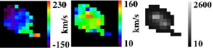
Figure 6: Kinematics of a major merger as derived from simulations of EAGLE observations at z$\sim$4, with 75mas/pixel, t_intg=24h and EE=34%. The velocity fields (first column), the velocity dispersion maps (second column), and the emission line flux maps (last column, units are in median counts per dit) are shown. The object size is 0.8 arcsec in diameter, which represents $\sim$0.12 kpc at z=4.

Even when the full kinematics of the galaxy or merger is not recovered, the total SNR is always larger that 5, down to 8hr of exposure time. We see that this partial information is sufficient to recover the dynamical nature of both the major merger and the rotating disk, for a large range of EE (see Fig. 9). Although based on a limited number of cases, this suggests that it is not mandatory to recover the full 2D kinematics to infer the dynamical nature of distant galaxies. The dynamical state of a galaxy is mostly reflected in its large scale motions, rather than in its small scale perturbations (see also Flores et al. 2006). This is why it appears sufficient to recover only part of the 2D information, providing that this information is reliable enough (i.e., recovered with enough SNR). We will discuss this point further in Sect. 8.1.

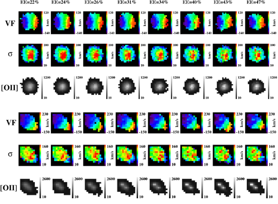
Figure 7: Kinematics of a rotating disk (three top lines) and a major merger (three lowest lines) as derived from simulations of EAGLE observations at z$\sim$4, with 75 mas pixel^-1 and t_intg=200h. The velocity fields (VF), the velocity dispersion maps ($\sigma$), and the emission line flux maps ([OII], units are in median counts per dit) are shown. Each column corresponds to a given EE in 0.15 arcsec, as indicated at the top.

Figure 8: Radius-average profile of the maximal SNR in the [OII] emission line of the rotating disk, obtained after 24hr (full lines) and 8hr (dotted lines) of exposure time. In each case, the upper curve is obtained for the highest EE (47%), and the bottom one for the smallest EE (22%). Error-bars account for the 1-sigma dispersion in SNR and positions within each ring of the profile. Only pixels having $SNR_{kin}>$3 have been considered to build the profile.

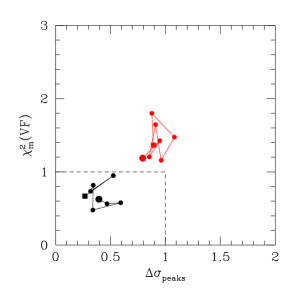
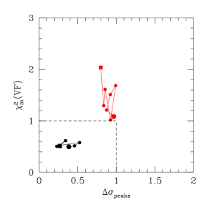
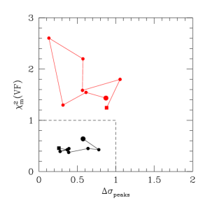
Figure 9: From left to right: Diagnostic diagram for identifying rotating disks in EAGLE simulations of z$\sim$4 galaxies with 75mas/pixel and t${}_{intg}\sim$200h, 24h, and 8h. Each point represents a different AO correction, from the worst one (EE=22%, see the biggest point) to the best one (EE=47%, see the bigger square). The black track corresponds to the rotating disk, and the red one to the major merger.

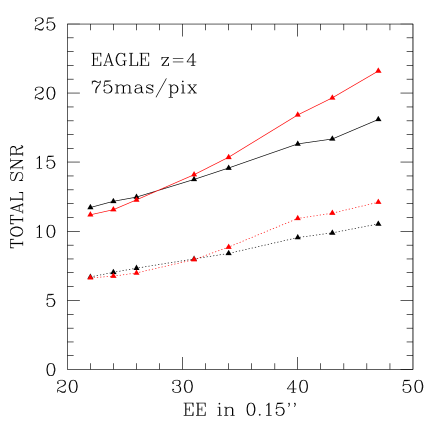
Figure 10: Flux-weighted SNR in the center of the emission line, integrated over the galaxy for EAGLE simulations with 75mas/pix and 24 or 8 hr of exposure times (respectively: full lines and dotted lines). The black curves correspond to the rotating disk, while the red ones correspond to the major merger.

7.2 The Design Requirements for FALCON on the VLT

We proceed as described in §3.6, and ran a set of simulations with a total integration time t_intg=200h (see Fig. 11). To distinguish a merger from a simple rotating disk in both the $\sigma$ and velocity maps, we find that a minimum $\sim$30% of EE (in 0.25 arcsec) is required. Again, this EE corresponds to a FWHM smaller than 2 pixels (see Fig. 5).

With 24hr of exposure time, the total SNR ranges between $\sim$6 and $\sim$11, and between $\sim$4 and $\sim$8 with 8hr, depending on the EE (see Fig. 14). Reaching a total SNR of 5 thus requires at least 8hr with a minimal EE of 30%, or more than 3hr, assuming an EE of 46%.

We find that recovering the full kinematic information requires at least 24hr of exposure time and an EE of 35% (see Fig. 12). Again, this EE corresponds to a PCT smaller than 50% (see Fig. 5), i.e., to a good “PSF contrast”. In a previous study, Assémat et al. (2007) found that 35% of EE was required for detecting the H$\alpha$ emission line at a 3$\sigma$ level. However, one can expect that for measuring higher moments of the emission line, i.e., the first and second moments, a larger SNR will be required. If the velocity measurement does not seem to be affected much by the SNR, the velocity dispersion clearly suffers from a too low SNR, since the two progenitors can hardly be directly identified in Fig 12, relying on velocity dispersion maps only.

With 8hr of integration time, it is possible to recover the true underlying nature of dynamics of high redshift galaxies, using the diagnostic diagram (see Fig. 13). However, a minimal EE of 26% and 35% are respectively necessary for integration times of 24 and 8h. However, the diagnostic diagram generally fails when the total SNR is smaller than $\sim$5 (see Fig. 14), confirming once again that 5 appears to be the lowest acceptable SNR.

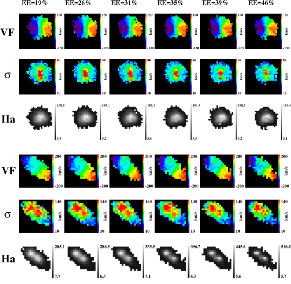
Figure 11: Kinematics of a rotating disk (three top lines) and a major merge (three lowest lines) as derived from simulations of FALCON observations at z$\sim$1.6, with t_intg=200h. For both objects, the velocity fields (VF), velocity dispersion maps ($\sigma$), and emission line maps (H$\alpha$, units are in median counts per dit) are shown. Each column corresponds to a given EE in 0.25 arcsec, as indicated at the top.

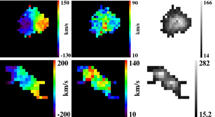
Figure 12: Kinematics of a rotating disk and major merger as derived from simulations of FALCON observations at z$\sim$1.6 (0.125 arcsec/pixel), with t_intg=24h and EE=35%. For both objects, the velocity fields (first column), velocity dispersion maps (second column), and emission line maps (third column, units are in median counts per dit) are shown. The objects size is 2 arcsec in diameter, which represents $\sim$0.24 kpc at z=1.6.

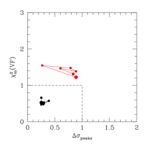
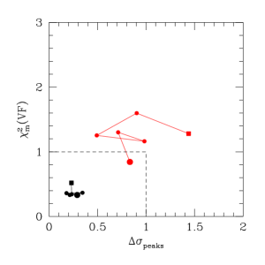
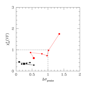
Figure 13: Diagnostic diagram for identifying rotating disks in FALCON simulations of z$\sim$1.6 galaxies with 125mas/pixel and t${}_{intg}\sim$200h, 24h, and 8h (from left to right). Each point represents a different AO correction, from the worst one (EE=19%, see the biggest point) to the best one (EE=46%, see the bigger square). The black track corresponds to the rotating disk, and the red one to the major merger.

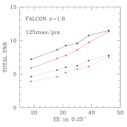
Figure 14: Total flux-weighted SNR over the galaxy for FALCON simulations with 24 and 8 hr of exposure times (respectively: full lines, dashed lines, and dotted lines). The black curves correspond to the rotating disk, while the red ones correspond to the major merger.

8 Discussion & Summary

8.1 Spatial “scale-coupling”: Influence of the pixel size for EAGLE

We also ran simulations of the EAGLE instrument concept for the E-ELT with a smaller pixel scale, 50 mas (see Fig. 16). FWHMs and PCTs are shown in Fig. 15. The two progenitors of the major merger can be clearly separated in both the $\sigma$ and the [OII] maps (see Fig. 16) with EE $>$15% (in 0.1 arcsec), which again corresponds to the EE where the FWHM becomes smaller than two pixels.

Figure 15: Top: FWHM vs. EE for the eight simulated EAGLE PSFs. The dotted line represents the diffraction limit on a 42m ELT in the H-band, i.e., $\lambda_{diff}(H)=0.008$ arcsec. The dashed lines shows when the FWHM becomes lower than 0.1 arcsec, i.e., twice the pixel size (under-sampling). Bottom: PCT vs. EE for the eight simulated EAGLE PSFs. The black line is a linear fit between FWHM et EE.

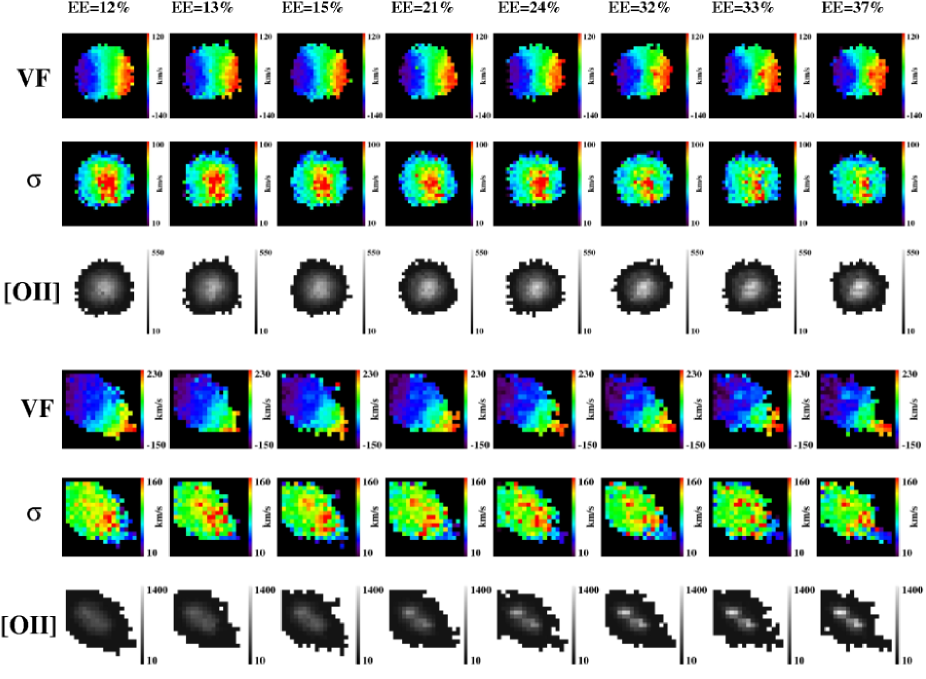
Figure 16: Kinematics of a rotating disk (three top lines) and a major merger (three lowest lines) as derived from simulations of EAGLE observations at z$\sim$4, with 50mas/pixel and t_intg=200h. The velocity fields (VF), the velocity dispersion maps ($\sigma$), and the emission line flux maps ([OII], units are in median counts per dit) are shown. Each column corresponds to a given EE in 0.1 arcsec, as indicated at the top.

As expected, the achieved total SNR at a given integration time and EE, is lower with a 50 mas pixel scale than with one of 75 mas pixel^-1 (see Fig. 18). Reaching a minimal total SNR of 5 requires at least 8hr of exposure time with an EE of 21%, or at least $\sim$3hr with a larger EE.

With 50 mas pixel^-1, we find that the low surface brightness tidal tail of the merger can be detected in t_intg=24h with at least 32% of EE. In contrast to the previous cases, this EE does not correspond to the one giving 50% of PCT: this condition now gives a much smaller EE (smaller than 10, see Fig. 15), which does not provide enough SNR to make this distinction (Fig. 18). With the 75 mas pixel^-1 scale, detecting the tidal tail required a total SNR of $\sim$15: this is roughly the total SNR that is now provided by 32% of EE with the 50 mas pixel^-1 scale. This is obviously related to subdividing the total flux of the tail into smaller and smaller sampling of a structure with a relatively smooth surface brightness distribution.

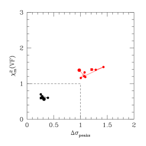
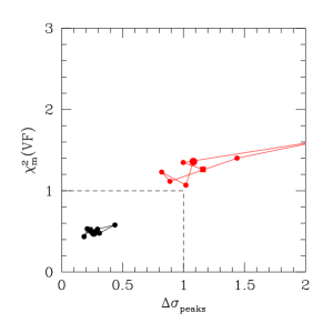
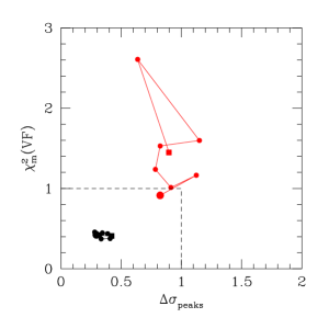
Figure 17: From left to right: Diagnostic diagram for identifying rotating disks in EAGLE simulations of z$\sim$4 galaxies with 50 mas pixel^-1 and t${}_{intg}\sim$200h, 24h, and 8h. Each point represents a different AO correction, from the worst one (EE=12%, see the biggest point) to the best one (EE=37%, see the bigger square). The black track corresponds to the rotating disk, and the red one to the major merger.

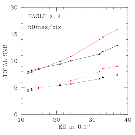
Figure 18: Total flux-weighted SNR over the galaxy for EAGLE simulations with 50mas.pix^-1 and 24 and 8 hr of exposure times (respectively: full lines, dashed lines, and dotted lines). The black curves correspond to the rotating disk, while the red ones correspond to the major merger.

Using the diagnostic diagram, it is possible to disentangle the major merger from the rotating disk with a pixel scale of 50 mas pixel^-1 (see Fig. 17). Again, the diagnostic diagram tends to fail when the total SNR is smaller than 5 (see Fig. 18).

The comparison of the 50 and 75 mas pixel^-1 scales reveals that the former does not bring significant more information compared to the latter, relatively to the goal of distinguishing between the major merger and the rotating disk. This is related to the fact that, as mentioned before, the dynamical state of a galaxy is reflected in its large scale motions, rather than in its small scale perturbations. Hence, having a very fine pixel scale does not provide any advantage in this respect, and might limit the SNR achievable for a given integration time. Obviously, such a conclusion depends on the spatial scale of the kinematic feature to be recovered: if one wants to recover smaller-scale kinematic details like, e.g., the precise rotation curve, or to detect clumps in distant disks, a finer spatial scale will be then preferable. This optimal “scale-coupling” between the IFU pixel scale and the spatial scale of the physical feature that one wants to recover using this IFU can be quantified by the ratio between the size of this feature (here, the galaxy diameter, as one wants to recover the large-scale rotation) and the size of the IFU resolution element. At z$\sim$4, this “scale-coupling” is found to be 5.3 using the 75 mas pixel^-1 scale, and 8, using the 50 mas pixel^-1 scale. In other words, our simulations suggest that a “scale-coupling” of 5.3 is already large enough to recover large-scale motions in z$\sim$4 galaxies. This is in line with 3D observations of z$\sim$0.6 galaxies with FLAMES/GIRAFFE, which provides a “scale-coupling” of about 3 (Flores et al. 2006; Yang et al. 2008): this is the minimum value necessary to ensure that each side of the galaxy is at least spatially sampled by the IFU at the Nyquist rate. Using this minimum ratio, one finds that a pixel scale of at least $\sim$130 mas is mandatory for studying large-scale motions in z$\sim$4 galaxies if they are simply scaled versions of nearby galaxies. On the other hand, the smallest pixel scale that can be used for a given scientific goal is limited by the achievable SNR at this scale, which is in turn constrained by the “PSF contrast” as discussed above in Sect. 7.

8.2 Influence of Telescope Diameter

As discussed previously, in most cases MOAO will provide 3D spectroscopy of distant galaxies with a spatial resolution limited by the IFU pixel scale, because MOAO essentially provides partial AO corrections. Everything else being equal, using a larger aperture telescope will then only influence the integration time needed to reach a given SNR, thanks to the larger collecting power of the primary mirror.

We show in Sect. 4, that an MOAO-fed IFS on the VLT could provide us with improved 2D-kinematics of z$\leq$2 galaxies. In Fig. 19, we show what the maps of the same galaxy would look like if observed with EAGLE on the E-ELT, using 50 mas pixel^-1 and t_intg=2h. Observations, with 24% of EE in 0.1 arcsec, provide a radial SNR profile comparable to the one obtained with FALCON after 24hr of exposure time and EE=39% (see Fig. 20). The E-ELT, equipped with an multi-object IFS, even with a low EE, would represent a huge improvement over 8-meter class telescopes, even equipped with future-generation MOAO-fed instruments. In return, the VLT, equipped with an MOAO-fed spectrograph would provide us with an important advancement in our knowledge of distant galaxies, increasing the number of spatial element of resolution from typically 2-3 to 13-20. This will be possible at the VLT with the Laser Guide Star Facility and SINFONI (pixel scale of 50 mas). This is already available with OSIRIS at Keck (with 20 to 100 mas pix^-1 AO-corrected; see Law et al. 2007; Wright et al. 2007). Other VLT second-generation NIR spectrographs, such as KMOS, will on the other hand allow us to gather further information on kinematics of 24 distant objects simultaneously, which is a great advantage in obtaining the statistical properties. However, it only has seeing limited performance over a 0.2 arcsec pixel^-1 scale. High spatial resolution integral field spectroscopy at the VLT will remain limited to single object observations. The number density of objects at z$\sim$1.4-2.5 is expected to be $\sim$ 9 per square arcmin, down to $I_{AB}\sim$25 (Steidel et al. 2004). KMOS will undoubtedly identify interesting objects amount the ensemble of z$\approx$2 galaxies with which to observe in more detail with AO-fed integral field spectrographs on 8-m class telescopes. However, an MOAO-fed spectrograph on currently available or a future extremely large telescope would optimally take advantage of these high target densities.

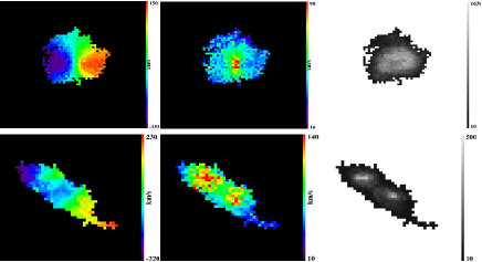
Figure 19: Kinematics of a rotating disk (first line) and a major merger (second line) as derived from EAGLE simulations at z$\sim$1.6, with t_intg=2h and EE=24% in 0.1 arcsec. For both objects, the velocity fields (first column), velocity dispersion maps (second column) and emission line maps (third column) are shown. Object size is 2 arcsec in diameter, which represents $\sim$0.24 arcsec at z=1.6.

Figure 20: Radius-average profile of the maximal SNR in the emission line, obtained after 24hr of exposure time and 39% of EE in 0.25 arcsec with FALCON (full lines), and after 8hr of exposure time and 24% of EE in 0.1 arcsec with EAGLE (dotted lines). Error-bars account for bootstrap uncertainties on the medians in SNR and positions within each ring of the profile.

8.3 Summary: High Level Design Requirements for MOAO systems

We first presented simulations of z$\sim$4 galaxies with very large SNRs, to focus on spatial smoothing effects due to partial corrections of the atmospheric turbulence by the MOAO system. In all cases, we find that the EE required to clearly identify the two components of the major merger considered in our simulations roughly corresponds the EE that provides us with a FWHM smaller than 2 pixels. For z=4 galaxies and using a 75mas pixel scale, this corresponds to an EE of $\sim$25% in 150 mas, while this condition translates into 15% in 100 mas with a 50mas pixel^-1 scale. At z=1.6, an EE of at least $\sim$30% within 0.25 arcsec is required, using a 0.125 arcsec pixel^-1 scale. Considering the spatial resolution only, (i.e., with an infinite SNR), these specifications are indications of the minimum we will realistically require to recover spatially resolved kinematic information on distant galaxies.

Considering the impact of signal to noise, if one wants to recover the full 2D kinematics of z=4 galaxies, at least 24 hr of integration time, and 34% of EE (in 0.15 arcsec, using the 75 mas pixel^-1 scale) are needed (or 32% in 0.1 arcsec using the 50 mas pixel^-1 scale). For z=1.6 FALCON simulations, at least 24 hr and 35% of EE in 0.25 arcsec are needed for recovering the full 2D kinematics in our simulations. When the SNR provided by the MOAO system is large enough, these EE roughly corresponds to a PCT smaller than 50%. This provides a good “PSF constrast” at a given spatial scale, which avoids significant amount of polluting light from adjacent spectra.

At lower SNR, the required EE naturally depends on the surface brightness of the faintest regions to be detected, as well as on the adopted pixel scale. The choice of the latter strongly depends on the scientific goal and the size of the features to be recovered by 3D spectroscopy: a good “scale-coupling” between them must provide a least a few spatial element of resolutions per important scale. Because the dynamical state of galaxies is mostly reflected in their large-scale motions, this means that only a few spatial element of resolution are needed per galaxy diameter: we performed additional simulations (not shown here) using another rotating disk with a less steep rotation curve (UGC6778, see Garrido et al. 2002), and found no quantitative difference in our results using this other rotating disk. Although based on a limited number of simulations, we find that indeed a spatial resolution element of 150 mas (pixel size of 75 mas) seems to be a good choice for recovering large scale motions, providing relatively large SNR with a “scale-coupling” $\sim$5.3 element of resolution per galaxy diameter (0.8 arcsec). At the 50mas pixel^-1 scale, a 42 m ELT will typically need 8 hr of exposure time to reach a SNR of at least 5 over a galaxy. Such a SNR allows us to use the diagnostic diagram as a useful tool to recover the dynamical nature of rotating disks and major mergers. Because of the much smaller collecting area of the VLT, this exercise is limited to 8 hr with at least 35% of EE in 0.25 arcsec, for z=1.6 galaxies. In this case, the “coupling factor” is 4. These results are consistent with previous studies at lower redshift (z$\sim$0.6), where the dynamical nature of galaxies have been recovered using GIRAFFE, with only 3 or so resolution elements (at 0.52 arcsec pixel^-1) across each galaxy.

9 Conclusion

We have developed software capable of end-to-end simulations of integral field spectrograph fed by an MOAO system. We have used this software to investigate a limited number of simulations in H-band, in order to give insights into how such MOAO-fed systems should perform on the VLT and the E-ELT. By requiring that the instrument is able to distinguish between a rotating disk and a major merger, we were able to constrain the required Ensquared Energy to be able to recover their large-scale motions. Separating the progenitors of the major merger requires only modest EE (15-26% at z=4 in a sample of 100-150mas; 30% at z=1.6 in 0.25 arcsec), but long exposure times ($\sim$24hr). Higher EEs are generally needed to recover the full 2D kinematics in our simulations, typically 35%. Provided that the total SNR is large enough over the galaxy (typically $\sim$ 5), it is possible to use more sophisticated methods, such as the diagnostic diagram introduced here, to distinguish between both types of objects, even at relatively low integration time for such distant objects (8 hrs). To generalize these results beyond what we described here, we have related these specifications to the concept of “PSF contrast”, which is the amount of polluting light from adjacent spectra and which drives the minimal EE at a given spatial scale. The choice of the latter is driven mostly by the “scale-coupling” which is the relative size of the IFU pixel and the size of the features that the observe wishes to recovered in the data cube. Distinguishing between a major merger and a disk, for example, can be largely done by investigating the large scale motions within a system, and a relatively coarse spatial resolution appears then to be sufficient. Given this situation, a pixel scale of 50-75 mas seems to be a relatively good choice, since it provides sufficient SNR in less time than a finer sampling and also has the advantage of relaxing the MOAO system requirements. More stringent requirements can be set by attempting to resolve and investigate structure in high redshift galaxies and that will be simulated in subsequent papers.

References

- Amram et al. (2002) Amram, P., Adami, C., Balkowski, C., et al. 2002, Ap&SS, 281, 393
- Assémat et al. (2007) Assémat, F., Gendron, E., & Hammer, F. 2007, MNRAS, 376, 287
- Beauvais & Bothun (1999) Beauvais, C., & Bothun, G. 1999, ApJS, 125, 99
- Bertin & Arnouts (1996) Bertin, E., & Arnouts, S. 1996, A&AS, 117, 393
- Beuzit et al. (2006) Beuzit, J.L., Feldt, M., Dohlen, K., et al. 2006, Msngr, 125, 29
- Bosma (1978) Bosma, A. 1978, PhD Thesis dissertation
- Bouwens et al. (2004) Bouwens, R.J., Illingworth, G.D., Blakeslee, J.P., et al. 2004, ApJ, 611, 1
- Cox et al. (2004) Cox, T.J., Primack, J., Jonsson, P., et al. 2004, ApJ, 607, 87
- Cox et al. (2006) Cox, T.J., Jonsson, P., Primack, J., et al. 2006, MNRAS, 373, 1013
- Dahlen et al. (2007) Dahlen, T., Mobasher, B., Dickinson, M., et al. 2007, ApJ, 654, 172
- Erb et al. (2006) Erb, D.K., Steidel, C.C., Shapley, et al. 2006, ApJ, 647, 128
- Ferguson et al. (2004) Ferguson, H.C., Dickinson, M., Giavalisco, M. et al. 2004, ApJ, 600, 107
- Finger et al. (2006) Finger, G., Garnett, J., Bezawada, N., et al. 2006, Nuclear Instruments & Methods in Physics Research A, 565, 241
- Flores et al. (2006) Flores, H., Hammer, F., Puech, M., et al. 2006, A&A, 455, 107
- Förster-Schreiber et al. (2006) Förster-Schreiber, N., Genzel, R., Lehnert, M.D., et al. 2006, ApJ, 645, 1062
- Fried (1981) Fried, D.L. 1981, JOSAA, 72, 52
- Fuentes-Carrera et al. (2004) Fuentes-Carrera, I., Rosado, M. Amram, P., et al. 2004, A&A, 415, 451
- Fusco et al. (1999) Fusco, T., Conan, J.-M., Michau, V., et al. 1999, SPIE Proc. Vol. 3763, 125
- Fusco et al. (2006) Fusco, T., Rousset, G., Sauvage, J.-F., et al., 2006, Opt. Expr., 14, 7515
- Garrido et al. (2002) Garrido, O., Marcelin, M., Amram, P. et al. 2002, A&A, 387, 821
- Goncharov et al. (2007) Goncharov, A.V., Devaney, N., & Dainty, C. 2007, Opt. Expr. 15, 1534
- Hammer et al. (1997) Hammer, F., Flores, H., Lilly, S.J., et al. 1997, ApJ, 481, 49
- Hammer et al. (2002) Hammer, F., Sayède, F., Gendron, E., et al. 2002, Proc. of the ESO workshop Scientific Drivers for ESO Future VLT/VLTI Instrumentation, 139
- Hammer et al. (2004) Hammer, F., Puech, M., Assémat, F., et al. 2004, Proc. SPIE Vol. 5382, 727
- Hammer et al. (2005) Hammer, F., Flores, H., Elbaz, D., et al. 2005, A&A, 430, 115
- Law et al. (2007) Law, D.R., Steidel, C.C., Erb, D.K., et al. 2007, ApJ, accepted, astro-ph/0707.3634
- Mannucci et al. (2001) Mannucci, F., Basile, F., Poggianti, B.M., et al. 2001, MNRAS, 326, 745
- Moretto et al. (2006) Moretto, G., Bacon, R., Cuby, J.-G., et al. 2006, Proc. SPIE Vol. 6269, 76
- Neichel et al. (2006) Neichel, B., Conan, J.-M., Fusco, T., et al. 2006, Proc. SPIE Vol. 6272, 58
- Puech & Sayède (2004) Puech, M., & Sayède, F., Proc. SPIE Vol. 5492, 303
- Puech et al. (2005) Puech, M., Chemla, F., Laporte, P., et al. 2005, Proc. SPIE Vol. 5903, 272
- Puech et al. (2006a) Puech, M., Hammer, F., Flores, H., et al. 2006, A&A, 455, 119
- Puech et al. (2006b) Puech, M., Flores, H., Hammer, F., et al. 2006, A&A, 455, 131
- Puech et al. (2008) Puech, M., Flores, H., Hammer, F., et al. 2008, A&A accepted, astro-ph/0803.3002
- Reddy et al. (2006) Reddy, N.A., Steidel, C.C., Erb, D.K., et al. 2006, ApJ, 653, 1004
- Roddier (1981) Roddier, F. 1981, Progress in Optics, 19, 281
- Sarzi et al. (2006) Sarzi, M., Falcon-Barroso, J., Davies, R.L., et al. 2006, MNRAS, 366, 1151
- Semelin & Combes (2005) Semelin, B., & Combes, F. 2005, A&A, 441, 55
- Steidel et al. (2004) Steidel, C.C., Shapley, A.E., Pettini, M., et al. 2004, ApJ, 604, 534
- Tallon & Foy (1990) Tallon, M. & Foy, R. 1990, A&A, 235, 549
- Tokovinin et al. (2001) Tokovinin, A. & Viard, E. 2001, JOSA, 18, 873
- Wright et al. (2007) Wright, S.A., Larkin, J.E., Barczys, M., et al. 2007, ApJ, 658, 78
- Yang et al. (2008) Yang, Y., Flores, H., Hammer, F., et al. 2008, A&A, 477, 789
- Yoshida et al. (2006) Yoshida, M., Shimasaku, K., Kashikawa, N., et al. 2006, ApJ, 653, 988