Loop series expansion with propagation diagrams

Abstract

The Bethe approximation is a successful method for approximating partition functions of probabilistic models associated with a graph. Recently, Chertkov and Chernyak derived an interesting formula called “Loop Series Expansion”, which is an expansion of the partition function. The main term of the series is the Bethe approximation while other terms are labelled by subgraphs called generalized loops. In this paper, we derive a loop series expansion of binary pairwise Markov random fields with “propagation diagrams”, which describe rules how “first messages” and “secondary messages” propagate. Our approach allows to express the loop series in the form of a polynomial with coefficients positive integers. Using the propagation diagrams, we establish a new formula that shows a relation between the exact marginal probabilities and their Bethe approximations.

1 Introduction

@ A Markov random field (MRF) associated with a graph is given by a joint probability distribution over a set of variables. In the associated graph, the nodes represent variables and the edges represent probabilistic dependence between variables. A typical example of a MRF is a Gibbs distribution of the Ising model on a finite lattice. The joint distribution is often given in an unnormalized form, and the normalization factor of a MRF is called a partition function.

The main topic of this paper is computation of the partition function and the marginal distributions of a MRF with discrete variables. This problem is in general computationally intractable for a large number of variables, and some approximation method is required. Among many approximation methods, the Bethe approximation [1] has attracted renewed interest of computer scientists; it is equivalent to Loopy Belief Propagation (LBP) algorithm [2, 3], which has been successfully used for many applications such as error correcting codes, inference on graphs, image processing, and so on [4, 5, 6].

Chertkov and Chernyak [7, 8] give a new and interesting formula called loop series expansion, which expresses the partition function in terms of a finite series. The first term is the Bethe approximation, and the others are labelled by so-called generalized loops. The Bethe approximation can be corrected with this formula, though summing up all the terms requires computational efforts exponential to the number of linearly independent cycles.

In this paper we propose an alternative diagram-based method for deriving the loop series expansion formula. In our approach, we define secondary messages, which are orthogonal to the messages used in the LBP algorithm, and show that they satisfy a set of rules as they propagate. For each node and edge, we associate parameters $\{\gamma_{i}\}$ and $\{\beta_{ij}\}$, respectively; $\gamma_{i}$ is related to the approximated marginal of a node $i$, and $\beta_{ij}$ to the approximated correlation of adjacent nodes $i$ and $j$. The loop series is represented by a polynomial of these variables with coefficients positive integers. This positivity is useful for deriving a bound on the number of generalized loops.

The main result of this paper is theorem 4, with which we can calculate the true marginal probabilities in terms of the beliefs at the convergence of the LBP, $\{\gamma_{i}\}$, and $\{\beta_{ij}\}$. The terms in the formula of the marginals depend on the topological structure of the graph.

This paper is organized as follows. In section 2, we briefly review the definition of pairwise MRF, the Bethe approximation and the LBP algorithm. In section 3, we characterize the Bethe approximation as the fixed points of the LBP and deduce the fixed point equation in theorem 1. In section 4, we define first and secondary messages, and study their propagation rules. These rules are fundamental tools for our analysis. In section 5, we derive the loop series formula, and compare it with the results of Chertkov and Chernyak. We deduce consequences of our representation of the expansion: the connection to the partition function of the Ising model (with uniform coupling constant and external field) and the upper bound on the number of generalized loops. In section 6, we prove an expansion formula for the true marginal probability, and provide some examples.

2 Bethe approximation and loopy belief propagation algorithm

2.1 Pairwise Markov random field

We introduce a probabilistic model considered in this paper, MRF of binary states with pairwise interactions. Let $G:=(V,E)$ be a connected undirected graph, where $V=\{1,\ldots,N\}$ is a set of nodes and $E\subset\{(i,j);1\leq i<j\leq N\}$ is a set of undirected edges. Each node $i\in V$ is associated with a binary space $\chi_{i}=\{\pm 1\}$. We make a set of directed edges from $E$ by $\vec{E}=\{(i,j),(j,i);(i,j)\in E\}$. The neighbours of $i$ is denoted by $N(i)\subset V$, and $d_{i}=|N(i)|$ is called the degree of $i$. A joint probability distribution on the graph $G$ is given by the form:

$$p(x)=\frac{1}{Z}\prod_{ij\in E}\psi_{ij}(x_{i},x_{j})\prod_{i\in V}\phi_{i}(x_{i}),$$ (1)

where $\psi_{ij}(x_{i},x_{j}):\chi_{i}\times\chi_{j}\rightarrow\mathbb{R}_{>0}$ and $\phi_{i}:\chi_{i}\rightarrow\mathbb{R}_{>0}$ are positive functions called compatibility functions. The normalization factor $Z$ is called the partition function. A set of random variables which has a probability distribution in the form of (1) is called a Markov random field (MRF) or an undirected graphical model on the graph $G$. This class of probability distributions is equivalent to the Ising model with arbitrary coupling constants and local magnetic fields. In traditional literatures of statistical physics, a graph $G$ is often given by an infinite lattice, but as per recent interest, especially in computer science, $G$ has an arbitrary topology with finite nodes.

Without loss of generality, univariate compatibility functions $\phi_{i}$ can be neglected because they can be included in bivariate compatibility functions $\psi_{ij}$. This operation does not affect the Bethe approximation and the LBP algorithm given below; we assume it as per the following.

2.2 Loopy belief propagation algorithm

The LBP algorithm computes the Bethe approximation of the partition function and the marginal distribution of each node with the message passing method [9, 2, 3]. This algorithm is summarized as follows.

1. Initialization:
   For all $(j,i)\in\vec{E}$, the message from $i$ to $j$ is a vector $m_{(j,i)}^{0}\in\large{\mathbb{R}}^{2}$. Initialize as

   $$m_{(j,i)}^{0}(x_{j})=1\quad\forall x_{j}\in\chi_{j}.$$ (2)

2. Message Passing:
   For each $t=0,1,\ldots$, update the messages by

   $$m^{t+1}_{(j,i)}(x_{j})=\omega\sum_{x_{i}\in\chi_{i}}\psi_{ji}(x_{j},x_{i})\prod_{k\in N(i)\backslash\{j\}}m^{t}_{(i,k)}(x_{i}),$$ (3)

   until it converges. Finally we obtain $\{m^{*}_{(j,i)}\}_{(j,i)\in\vec{E}}$.

3. Approximated marginals and the partition function are computed by the following formulas:

   $$b_{i}(x_{i}):=\omega\prod_{j\in N(i)}m^{*}_{(i,j)}(x_{i}),$$ (4)

   $$b_{ji}(x_{j},x_{i}):=\omega\quad\psi_{ji}(x_{j},x_{i})\prod_{k\in N(j)\backslash\{i\}}m^{*}_{(j,k)}(x_{j})\prod_{k^{\prime}\in N(i)\backslash\{j\}}m^{*}_{(i,k^{\prime})}(x_{i}),$$ (5)

   $$\log Z_{B}:=\sum_{(j,i)\in{E}}\sum_{x_{j},x_{i}}b_{ji}(x_{j},x_{i})\log\psi_{ji}(x_{j},x_{i})-\sum_{(j,i)\in{E}}\sum_{x_{j}x_{i}}b_{ji}(x_{j},x_{i})\log b_{ji}(x_{j},x_{i})$$

   $$+\sum_{i\in V}(d_{i}-1)\sum_{x_{i}}b_{i}(x_{i})\log b_{i}(x_{i}),$$ (6)

   where $\omega$ are appropriate normalization constants, $b_{i}$ are called beliefs, and $Z_{B}$ is called the Bethe approximation of the partition function.

In step (2), there is ambiguity as to the order of updating the messages. We do not specify the order, because the fixed points of LBP algorithm do not depend on its choice. Note that this LBP algorithm does not necessarily converge, and there may be more than one fixed points unless the interactions are sufficiently weak [10].

3 Fixed point equation of LBP

When LBP converges, any converged messages $\{m^{*}_{(j,i)}\}_{(j,i)\in\vec{E}}$ satisfy a certain equation shown in theorem 1. By this theorem we show that the converged messages can be normalized simultaneously and we define $\{\mu_{(j,i)}\}_{(j,i)_{\in\vec{E}}}$ called first messages.

3.1 Graph operations

First, we remark that we can always add a new node without changing the marginals and beliefs of the others. For an edge $(i,j)$, we can add a node $k$ between $i$ and $j$ as in figure 2 with new compatibility functions $\psi_{ik},\psi_{kj}$ satisfying

$$\psi_{ij}(x_{i},x_{j})=\sum_{x_{k}}\psi_{ik}(x_{i},x_{k})\psi_{kj}(x_{k},x_{j}).$$ (7)

This operation will be used implicitly many times in this paper. Adding new nodes, if necessary, we can always assume that “there are sufficiently many nodes of degree two”.

Next we define a graph $\hat{G}$ by $G$. Let $L:=|E|-|V|+1$, the number of linearly independent cycles. Cutting and duplicating $L$ nodes of degree two appropriately, we obtain a connected tree $\hat{G}$, since we assume that there are sufficiently many nodes of degree two [11]. See figure 2. Renumbering the nodes of $V$, we assume that the cut nodes are numbered by $\{1,\ldots,L\}$. We define $\hat{G}=(\hat{V},\hat{E})$ by $\hat{V_{1}}=\{1,\ldots,L\}\cup\{\bar{1},\ldots,\bar{L}\}$, $\hat{V_{2}}=\{L+1,\ldots,N\}$ and $\hat{V}=\hat{V_{2}}\cup\hat{V_{1}}$. $\hat{E}$ is also naturally defined. We call $\hat{V}_{1}$ leaf nodes.

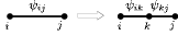
Figure 1: A new node can be added on an edge.

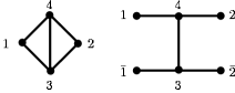
Figure 2: An example of $G$ and $\hat{G}$.

3.2 Belief propagation equations

Using the converged messages $\{m^{*}_{(j,i)}\}$, we define messages coming into the leaf nodes of the graph $\hat{G}$ as follows. Let $s$ be a cut node with the neighbour $N(s)=\{u,v\}$ in $G$, and let $(s,v),(\bar{s},u)\in\hat{E}$ be the edges at the duplicated nodes We define $\mu_{{s}}\propto m^{*}_{(s,u)}$, $\mu_{\bar{s}}\propto m^{*}_{(s,v)}$ and normalize them by $\sum_{x_{s}}\mu_{s}(x_{s})\mu_{\bar{s}}(x_{s})=1$. Generalizations of the transfer matrices are defined by

$$T^{x_{1},\ldots,x_{L}}_{\quad x_{\bar{1}},\ldots,x_{\bar{L}}}=\sum_{x_{L+1},\ldots,x_{N}}\prod_{(i,j)\in\hat{E}}\psi_{ij}(x_{i},x_{j}),$$ (8)

$${T_{s}}^{x_{s}}_{\quad{x_{\bar{s}}}}=\sum_{x_{1},\ldots,x_{s-1},\atop x_{s+1},\ldots,x_{L}}\sum_{x_{\bar{1}},\ldots,x_{\bar{s-1}},\atop x_{\bar{s+1}},\ldots,x_{\bar{L}}}T^{x_{1},\ldots,x_{L}}_{\quad x_{\bar{1}},\ldots,x_{\bar{L}}}\prod^{L}_{m=1\atop m\neq s}\mu_{m}(x_{m})\mu_{\bar{m}}(x_{\bar{m}}).$$ (9)

Since $\{m^{*}_{(j,i)}\}$ is the convergence point of the LBP algorithm, it is easy to see that there is $\alpha_{s}>0$ that satisfies $\alpha_{s}\mu_{s}(x_{s})=\sum_{{x_{s}}^{\prime}}{T_{s}}^{{x_{s}}^{\prime}}_{\quad{x_{s}}}\mu_{s}({x_{s}}^{\prime}).$ The following theorem states that all $\alpha_{s}$ are equal to $Z_{B}$.

Theorem 1.

for $s=1,\ldots,L$

$$Z_{B}\mu_{s}(x_{\bar{s}})=\sum_{{x_{s}}}{T_{s}}^{{x_{s}}}_{\quad{x_{\bar{s}}}}\mu_{s}({x_{s}})\quad x_{\bar{s}}\in\chi_{\bar{s}},$$ (10)

$$Z_{B}\mu_{\bar{s}}(x_{s})=\sum_{{x_{\bar{s}}}}{T_{s}}^{{x_{s}}}_{\quad{x_{\bar{s}}}}\mu_{\bar{s}}({x_{\bar{s}}})\quad {x_{s}}\in\chi_{{s}}.$$ (11)

Proof.

From $\alpha_{s}\mu_{s}(x_{s})=\sum_{{x_{s}}^{\prime}}{T_{s}}^{{x_{s}}^{\prime}}_{\quad{x_{s}}}\mu_{s}({x_{s}}^{\prime})$, $\alpha_{s}$ and $\alpha_{\bar{s}}$ are the Perron-Frobenius eigenvalues of the matrix ${T_{s}}^{{x_{s}}^{\prime}}_{\quad{x_{s}}}$ and its transpose, respectively. Therefore $\alpha_{s}=\alpha_{\bar{s}}$ for $1\leq s\leq L$. Next, we prove $\alpha_{s}=\alpha_{l}$ for $1\leq s,l\leq L$. As we normalize $\sum_{x_{s}}\mu_{s}(x_{s})\mu_{\bar{s}}(x_{s})=1$,

$$\alpha_{s} =\sum_{x_{s}}\{\alpha_{s}\mu_{s}(x_{s})\}\mu_{\bar{s}}(x_{s})$$

$$=\sum_{x_{1}\ldots,x_{L}}\sum_{x_{\bar{1}}\ldots,x_{\bar{L}}}T_{\quad x_{\bar{1}},\ldots,x_{\bar{L}}}^{x_{1},\ldots,x_{L}}\prod^{L}_{m=1}\mu_{m}(x_{m})\mu_{\bar{m}}(x_{\bar{m}})$$

$$=\alpha_{l},$$

which shows $\alpha_{l}=\alpha_{s}=\alpha$. Finally we prove $\alpha=Z_{B}$. By dividing some $\psi$ function by $\alpha$ from the first, we can assume that $\alpha=1$. Then it is sufficient to prove $\log Z_{B}=0$. By distributing the messages $\{\mu_{s}\}_{s\in\hat{V}_{1}}$ on the tree $\hat{G}$ from its leaf nodes $\hat{V}_{1}$ without normalization, we define a message $\mu_{(j,i)}$ at each edge $(j,i)\in\vec{E}$. Because $\hat{G}$ is a tree, the messages $\{\mu_{(j,i)}\}_{(j,i)\in\vec{E}}$ are uniquely defined step by step from the leaf nodes. By the assumption $\alpha=1$, we have $\mu_{s}=\mu_{(s,u)}$. Therefore,

$$\mu_{(j,i)}(x_{j})=\sum_{x_{i}\in\chi_{i}}\psi_{ji}(x_{j},x_{i})\prod_{s\in N(i)\backslash\{j\}}\mu_{(i,s)}(x_{i}),\qquad{}^{\forall}(j,i)\in\vec{E}.$$ (12)

By the relation

$$\sum_{x_{i}}\prod_{j\in N(i)}\mu_{(i,j)}(x_{i})=\sum_{x_{1}\ldots,x_{L}}\sum_{x_{1}\ldots,x_{L}}T_{\quad x_{\bar{1}},\ldots,x_{\bar{L}}}^{x_{1},\ldots,x_{L}}\prod^{L}_{m=1}\mu_{m}(x_{m})\mu_{\bar{m}}(x_{\bar{m}})=1,$$ (13)

we obtain

$$b_{i}(x_{i})=\prod_{j\in N(i)}\mu_{(i,j)}(x_{i}),$$ (14)

$$b_{ji}(x_{j},x_{i})=\psi_{ji}(x_{j},x_{i})\prod_{s\in N(j)\backslash\{i\}}\mu_{(j,s)}(x_{j})\prod_{s^{\prime}\in N(i)\backslash\{j\}}\mu_{(i,s^{\prime})}(x_{i}).$$ (15)

The assertion follows from putting (14) and (15) into the definition of $Z_{B}$ (6). ∎

As used in the proof of above theorem, the normalization $Z_{B}=1$ is convenient; in the rest of this paper we assume the following.

Assumption.

By normalizing one of $\{\psi_{ij}\}$, we assume $Z_{B}=1$.

In the proof of the above theorem, we defined the messages $\mu_{(j,i)}\propto m^{*}_{(j,i)}$ satisfying (12),(14) and (15). We call $\mu_{(j,i)}$ (normalized) first messages. While these conditions are similar to (3),(4) and (5), an important difference is disappearance of the normalization constants $\omega$. By the above assumption, the first messages satisfy (12). Notice that we define $\{\mu_{(j,i)}\}_{(j,i)\in\vec{E}}$ on the graph $G$, not only on the graph $\hat{G}$.

This equation is a generalization of recursive expression for calculating free energy of the Bethe lattice [12]. For each fixed point of the LBP algorithm $\{m^{*}_{(j,i)}\}$, there is a solution of equation (10),(11). On the other hand, for each solution of (10) and (11), there is a LBP fixed point.

4 Propagation diagrams

We proved in the previous section, if we normalize $\sum_{x_{s}}\mu_{s}(x_{s})\mu_{\bar{s}}(x_{s})=1$, the Bethe-approximated partition function is given by

$$Z_{B}=\sum_{x_{{1}}\ldots,x_{{L}}}\sum_{x_{\bar{1}}\ldots,x_{\bar{L}}}T_{\quad x_{\bar{1}},\ldots,x_{\bar{L}}}^{x_{1},\ldots,x_{L}}\prod^{L}_{m=1}\mu_{m}(x_{m})\mu_{\bar{m}}(x_{\bar{m}}),$$ (16)

while the true partition function is

$$Z=\sum_{x_{{1}}\ldots,x_{{L}}}T_{\quad x_{{1}},\ldots,x_{{L}}}^{x_{1},\ldots,x_{L}}=\sum_{x_{{1}}\ldots,x_{{L}}}\sum_{x_{\bar{1}}\ldots,x_{\bar{L}}}T_{\quad x_{\bar{1}},\ldots,x_{\bar{L}}}^{x_{1},\ldots,x_{L}}\prod^{L}_{m=1}\delta_{x_{m},x_{\bar{m}}}.$$ (17)

Let us define vectors $\nu_{s}$ and $\nu_{\bar{s}}$ for $s=1,\ldots,L$ as to satisfy

$$\sum_{x_{s}}\mu_{s}(x_{s})\nu_{\bar{s}}(x_{s})=0,\quad\sum_{x_{s}}\mu_{\bar{s}}(x_{s})\nu_{{s}}(x_{s})=0,\quad\sum_{x_{s}}\nu_{s}(x_{s})\nu_{\bar{s}}(x_{s})=1.$$ (18)

Then, we have a decomposition of the unit matrix

$$\delta_{x_{s},x_{\bar{s}}}=\mu_{s}(x_{s})\mu_{\bar{s}}(x_{\bar{s}})+\nu_{s}(x_{s})\nu_{\bar{s}}(x_{\bar{s}}).$$ (19)

We can expand (17) using (19) in a sum of $2^{L}$ terms. The first term is obviously the Bethe approximated partition function (16). But the explicit form of the remaining $2^{L}-1$ terms is not obvious. In this section we define secondary messages $\{\nu(i,j)\}_{(i,j)\in\vec{E}}$ and derive rules, which describe how these messages propagate, for deriving the remaining terms.

4.1 Definition of secondary messages

By splitting nodes as in figure 3, any graphs can be transformed so that every node is of degree at most three. We make the compatibility functions of new edges infinitely strong: $\psi_{ij}(x_{i},x_{j})=\delta_{x_{i},x_{j}}$. This change does not affect the fixed points of LBP algorithm, hence the Bethe approximation. In subsections 4.1 and 4.2 we assume that the graph $G$ has undergone this transformation. The same transformation also appears in [13] and [14]. The first messages $\mu$ are defined on this transformed graph.

Figure 3: A node of degree $n$ can be split into $n-2$ nodes of degree 3.

We define “secondary messages” $\{\nu_{(i,j)}\}$ on the transformed graph using $\{\mu_{(i,j)}\}$. First, let $j$ be a node of degree two such that at least one adjacent node, denoted by $k$, has degree two (figure 5). We define $\nu$ at the node $j$ by the following conditions:

$$\sum_{x_{j}}\nu_{(j,i)}(x_{j})\mu_{(j,k)}(x_{j})=0,\quad\sum_{x_{j}}\mu_{(j,i)}(x_{j})\nu_{(j,k)}(x_{j})=0,$$ (20)

$$\sum_{x_{j}}\nu_{(j,i)}(x_{j})\nu_{(j,k)}(x_{j})=1.$$ (21)

Similarly, let $j$ be a node of degree two such that at least one adjacent node, denoted by $i$, has degree two (figure 5). We define $\nu$ at node $j$ by the following conditions:

$$\sum_{x_{j}}\nu_{(j,i)}(x_{j})\mu_{(j,k)}(x_{j})\mu_{(j,l)}(x_{j})=0,\quad\sum_{x_{j}}\mu_{(j,i)}(x_{j})\nu_{(j,k)}(x_{j})\mu_{(j,l)}(x_{j})=0,$$

$$\sum_{x_{j}}\mu_{(j,i)}(x_{j})\mu_{(j,k)}(x_{j})\nu_{(j,l)}(x_{j})=0,$$ (22)

$$\sum_{x_{j}}\nu_{(j,i)}(x_{j})\nu_{(j,k)}(x_{j})\mu_{(j,l)}(x_{l})=1,\quad\sum_{x_{j}}\mu_{(j,i)}(x_{j})\nu_{(j,k)}(x_{j})\nu_{(j,l)}(x_{j})=1,$$

$$\sum_{x_{j}}\nu_{(j,i)}(x_{j})\mu_{(j,k)}(x_{j})\nu_{(j,l)}(x_{j})=1.$$ (23)

These conditions determine $\nu_{(j,i)}$ uniquely up to a scalar factor at nodes of degree two, and up to sign at nodes of degree three. We assume that the first component $\nu_{(i,j)}(+)$ is negative without loss of generality.

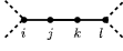
Figure 4: Node $j$ is degree 2.

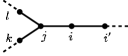
Figure 5: Node $j$ is degree 3, node $i$ is degree 2.

The above relations and $\sum_{x_{j}}\prod_{i\in N(j)}\mu_{(j,i)}(x_{j})=1$ (13) are pictorially summarized in figure 6. These cases are sufficient because we can add a node of degree two at any edge if necessary. We call such diagrams propagation diagrams. The blue dashed and the light red arrows express $\mu$ and $\nu$, respectively.

A condition which is similar to (20) and (22) is imposed in [15] to deduce the update rule of the LBP algorithm, though they consider a graphical model with variables on the edges.

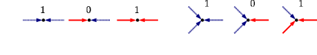
Figure 6: Rules at degree 2 and 3 nodes.

4.2 Propagation rules

The rules depicted in figure 6 describe what happens when messages collide at a node. The next two lemmas show how first and secondary messages propagate.

Lemma 1.

See figure 5. Suppose nodes $j$ and $k$ are of degree 2. Then, there is $\beta_{jk}\in\mathbb{R}$ such that

$$\beta_{jk}\nu_{(j,k)}(x_{j})=\sum_{x_{k}}\psi_{jk}(x_{j},x_{k})\nu_{(k,l)}(x_{k}),\qquad\beta_{jk}\nu_{(k,j)}(x_{k})=\sum_{x_{j}}\psi_{kj}(x_{k},x_{j})\nu_{(j,i)}(x_{j}).$$ (24)

Proof.

Using (12) and (20), $\sum_{x_{j},x_{k}}\mu_{(j,i)}(x_{j})\psi_{(j,k)}(x_{j},x_{k})\nu_{(k,l)}(x_{k})=\sum_{x_{k}}\mu_{(k,j)}(x_{k})\nu_{(k,l)}(x_{k})=0$. Hence $\sum_{x_{k}}\psi_{jk}(x_{j},x_{k})\nu_{(k,l)}(x_{k})\propto\nu_{(j,k)}(x_{j})$. The proportion is equal in the both directions $(j,k)$ and $(k,j)$ because of the condition (21). ∎

Next we proceed to a degree three node.

Lemma 2.

See figure 5. Suppose node $j$ is of degree three and $i$ is of degree two. Then, there is $\beta_{ji}\in\mathbb{R}$ such that

$$\beta_{ji}\nu_{(j,i)}(x_{j})=\sum_{x_{i}}\psi_{ji}(x_{j},x_{i})\nu_{(i,{i}^{\prime})}(x_{i}),$$ (25)

$$\beta_{ji}\nu_{(i,j)}(x_{i})=\sum_{x_{j}}\psi_{ji}(x_{j},x_{i})\nu_{(j,l)}(x_{j})\mu_{(j,k)}(x_{j}),$$ (26)

$$\beta_{ji}\nu_{(i,j)}(x_{i})=\sum_{x_{j}}\psi_{ji}(x_{j},x_{i})\mu_{(j,l)}(x_{j})\nu_{(j,k)}(x_{j}).$$ (27)

Proof.

We can show in the same way as the previous lemma. ∎

These lemmas say that the secondary messages $\nu$ propagate with rate $\beta$ for both directions, though the first messages $\mu$ propagate without variation in scales. Equations (26) and (27) hold when the adjacent nodes $i$ and $j$ have degree three as in figure 8. We associate numbers $\beta_{ij}$ for all undirected edges in $E$. Propagation diagrams of these results are summarized in figure 7.

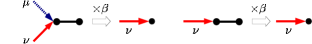
Figure 7: Propagation rules.

4.2.1 Two more rules

In addition to the rules in figure 6, we have to give a rule for the case in which three secondary messages $\nu$ collide at a node.

Lemma 3.

Let $N(j)=\{i,k,l\}$, then

$$\quad\sum_{x_{i}}\nu_{(j,i)}(x_{j})\nu_{(j,k)}(x_{j})\nu_{(j,l)}(x_{j})=\frac{1}{\sqrt{b_{j}(+)b_{j}(-)}}(b_{j}(+)-b_{j}(-))=:\gamma_{j}.$$ (28)

Proof.

We need direct computation of the message vectors. By the orthogonal condition (22), $\nu_{(j,i)}$, $\nu_{(j,k)}$ and $\nu_{(j,l)}$ are determined up to scalar factors. The scales are determined by (23). Since we assume the first components of $\nu$ are negative, $\nu$ must have the following form:

$$\nu_{(j,i)}(x_{j})=-x_{j}\sqrt{\frac{\mu_{(j,i)}(1)\mu_{(j,i)}(-1)}{\mu_{(j,k)}(1)\mu_{(j,k)}(-1)\mu_{(j,l)}(1)\mu_{(j,l)}(-1)}}\mu_{(j,k)}(-x_{j})\mu_{(j,l)}(-x_{j}).$$ (29)

From (14) the result follows. ∎

We use the next lemma when we split a node as in figure 3

Lemma 4.

See figure 8. If the nodes $j$ and $i$ are of degree three and $\psi_{i,j}{(x_{i},x_{j})}=\delta_{x_{i},x_{j}}$, then $\beta_{ij}=1$.

Proof.

By (27), (29) and the remark after lemma 2,

$$\beta_{ij}\nu_{(i,j)}(x_{i}) =\sum_{x_{j}}\psi_{ij}(x_{i},x_{j})\mu_{(j,l)}(x_{j})\nu_{(j,k)}(x_{j})$$

$$=\mu_{(j,l)}(x_{i})\nu_{(j,k)}(x_{i})$$

$$=-x_{i}\sqrt{\frac{\mu_{(j,k)}(1)\mu_{(j,k)}(-1)\mu_{(j,l)}(1)\mu_{(j,l)}(-1)}{\mu_{(j,i)}(1)\mu_{(j,i)}(-1)}}\mu_{(j,i)}(-x_{i}).$$

Since $\mu_{(j,i)}(x_{i})=\mu_{(i,l^{\prime})}(x_{i})\mu_{(i,k^{\prime})}(x_{i})$ and $\mu_{(i,j)}(x_{i})=\mu_{(j,l)}(x_{i})\mu_{(j,k)}(x_{i})$, we can show $\beta_{ij}=1$ by using (29) for $(i,j)$. ∎

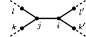
Figure 8: Node $j$ and $i$ have degree three.

4.3 At general nodes

We have defined $\nu$ on the transformed graph $G_{T}=(V_{T},E_{T})$ in which the degree of every node is at most three. By shrinking added edges, we define $\nu$ on the original graph $G=(V,E)$. In other words the injection $\vec{E}\rightarrow\vec{{E}_{T}}$ induces the messages on the original graph from the transformed graph. At each node of the original graph, we show that the following theorem holds. This theorem generalizes the rules in figure 6 and lemma 3.

Theorem 2.

Let $j\in V$ and $N(j)=\{i_{1},\ldots,i_{d_{j}}\}$. Then, we have

$$f_{n}(\gamma_{j})=\sum_{x_{j}}\prod_{s=1}^{n}\nu_{(j,i_{s})}(x_{j})\prod_{t=1}^{d_{j}-n}\mu_{(j,i_{n+t})}(x_{j}),$$ (30)

where $\{f_{n}(x)\}_{n=0}^{\infty}$ is a set of polynomials defined inductively by the relations $f_{0}(x)=1,f_{1}(x)=0$ and $f_{n+1}(x)=xf_{n}(x)+f_{n-1}(x)$.

Proof.

We can reduce to the case of $n=d_{j}$ by splitting node $j$ and using the propagation rules in figure 7. See figure 9 for example. The proof is done by induction; the cases of $n=1,2,3$ is obtained by definition. In the case of $n$ we split the node $j$ into $j^{\prime}$ and $j^{\prime\prime}$ where $2$ and $n-2$ secondary messages join at $j^{\prime}$ and $j^{\prime\prime}$, respectively. Adding a node $k$ between $j^{\prime}$ and $j^{\prime\prime}$, we use the relation $\mu_{(k,j^{\prime})}(x_{k})\mu_{(k,j^{\prime\prime})}({x_{k}}^{\prime})+\nu_{(k,j^{\prime})}(x_{k})\nu_{(k,j^{\prime\prime})}({x_{k}}^{\prime})=\delta_{x_{k},{x_{k}}^{\prime}}$. By lemma 4 and the induction hypothesis, we obtain $f_{n}(\gamma_{j})=f_{2}(\gamma_{j})f_{n-2}(\gamma_{j})+f_{3}(\gamma_{j})f_{n-1}(\gamma_{j})$. The assertion follows from the definition of the polynomials $f_{n}$. Figure 10 illustrate this procedure. ∎

It is surprising that the right hand side is determined by the value $\gamma_{j}$ which depends only on the belief $b_{j}$, while the messages $\mu_{(j,i_{s})}$ and $\nu_{(j,i_{s})}$ are not determined by $b_{j}$.

In this section we have derived a set of rules. In addition to the diagrams to show the rules, diagrams in which these rules are successively applied are also called propagation diagrams.

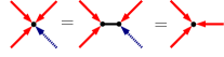
Figure 9: Reduction to the case of $n=d_{j}$.

Figure 10: Derivation of the inductive relation in the case of $n=4$.

4.4 In the case of one dimensional systems

In the case of one dimensional spin systems, results of section 3 and 4 are reduced to easy observations. Let the graph $G$ be a cycle of length $N$. We cut the node $1$ as discussed in section 3.1 to obtain a string. The partition function is

$$Z=\sum_{x_{1}=\pm 1}T^{x_{1}}_{\quad x_{\bar{1}}}$$ (31)

where the transfer matrix $T=T_{1}$ is defined by (8) and (9). Therefore $Z$ is equal to the sum of the first and second eigenvalues of the matrix $T$. By theorem 1, the first messages $\mu_{1}$ and $\mu_{\bar{1}}$ are the first right and left eigenvectors of the transfer matrix, where the first eigenvalue is $Z_{B}$. By lemma 1, we see that $\nu_{1}$ and $\nu_{\bar{1}}$ are the second right and left eigenvectors, and the second eigenvalue is $Z_{B}\prod\beta_{ji}$. The conditions of (20) are regarded as orthogonality of eigenvectors. The results of these sections are a generalization to the transfer tensor associated with more complicated graphs with nodes of degree three.

5 Loop series expansion formula

5.1 Derivation of loop series expansion formula

Let $G=(V,E)$ be a graph, and $D$ be a subset of the edge-set $E$. An edge-induced subgraph of $D$ is a subgraph of the graph $G$ whose edge-set is $D$ and whose node-set consists of all nodes that are incident with at least one edge in $D$.

We are now ready to prove the expansion formula of the partition function.

Theorem 3.

For each solution of (10),(11), define $\{\beta_{ij}\},\{\gamma_{i}\}$ by the above lemmas. Then the following expansion formula holds.

$$Z=Z_{B}(1+\sum_{\phi\neq C\in\mathcal{G}}r(C)),$$ (32)

$$r(C):=\prod_{ij\in{E}_{C}}\beta_{ij}\prod_{i\in V_{C}}f_{d_{i}(C)}(\gamma_{i}),$$

Where $\mathcal{G}$ is the set of all edge-induced subgraphs of $G$ and $C=(V_{C},E_{C})$.

Proof.

Adding a node $k$ on each edge $(i,j)$ of $G$, we expand the partition function by the relation $\mu_{(k,i)}(x_{k})\mu_{(k,j)}({x_{k}}^{\prime})+\nu_{(k,i)}(x_{k})\nu_{(k,j)}({x_{k}}^{\prime})=\delta_{x_{k},{x_{k}}^{\prime}}$. We have $2^{|E|}$ terms in this expansion, because for each edge $(i,j)$ there is a choice: $\mu_{(k,i)}(x_{k})\mu_{(k,j)}({x_{k}}^{\prime})$ or $\nu_{(k,i)}(x_{k})\nu_{(k,j)}({x_{k}}^{\prime})$. If we regard the $\nu$-edges as a edge-set, each term can be identified with an edge-induced graph. By theorem 2 and lemma 1 and 2, the term corresponding to $C$ is equal to $r(C)$. ∎

Since $f_{1}(x)=0$, $C$ makes a contribution to the sum only if $C$ does not have a node of degree one in $C$. Such $C$ is called a generalized loop. In the case that $G$ is a tree, there is no generalized loop, therefore $Z=Z_{B}$. This is well-known [9].

Note that $f_{n}(0)=1$ if $n$ is even, and $f_{n}(0)=0$ if $n$ is odd. If $\gamma_{i}=0$ for all $i\in V$, only generalized loops with even degrees contribute to the sum. This is reminiscent of the high temperature expansion of the Ising model without magnetic field. We further discuss this point in section 5.3. In addition, if the graph is planar, these terms are summed by a single Pfaffian [13, 14].

We can choose and expand some of the edges step by step with propagation diagrams as in A.1, while we expand at all edges in the above proof.

Let $\Theta(\{\beta_{ij}\},\{\gamma_{i}\}):=1+\sum_{\phi\neq C\in\mathcal{G}}r(C)$ . This is a polynomial of indeterminates $\{\beta_{ij}\}$ and $\{\gamma_{i}\}$, and its coefficients are positive integers, because $f_{n}(x)$ are polynomials with coefficients positive integers. We can assign other quantities to nodes and edges such as $\{m_{i}\}$ and $\{\tau_{ij}\}$ discussed later in section 5.2, and represent the formula in different manner with these quantities, but such assignment may cause large positive and negative coefficients. Advantage of using $\gamma$ and $\beta$ is that the coefficients are not huge because they are all positive and the total sum is determined by $L$ as discussed later in 5.4.2. Note that the method of propagation diagrams gives an algorithm for computing $\Theta$.

The messages $\mu$ and $\nu$ are explicitly given if we change the compatibility functions. By the definitions of the beliefs (4) and (5), we see that

$$\prod_{(i,j)\in E}\psi_{ij}(x_{i},x_{j})\propto\prod_{(i,j)\in E}b_{ij}(x_{i},x_{j})\prod_{i\in V}\frac{1}{{b_{i}(x_{i})}^{d_{i}-1}}.$$ (33)

Therefore, we can retake compatibility functions as

$$\psi_{ij}(x_{i},x_{j})=\frac{b_{ij}(x_{i},x_{j})}{{b_{i}(x_{i})}^{(d_{i}-1)/d_{i}}{b_{j}(x_{j})}^{(d_{j}-1)/d_{j}}}$$ (34)

without changing the joint probability distribution. Moreover, this does not cause any change to the result of the LBP algorithm, namely beliefs. In the rest of section 5.1 and section 5.2, we assume this representation of compatibility functions. By (12), for all $(j,i)\in\vec{E}$ the first messages have the following forms: $\mu_{(j,i)}(x_{j})=b_{j}(x_{j})^{1/{d_{j}}}$. The secondary messages are determined by theorem 2 as

$$\nu_{(j,i)}(x_{j})=\frac{-x_{j}b_{j}(-x_{j})^{(d_{j}-1)/d_{j}}}{b_{j}(+)^{(d_{j}-2)/2d_{j}}b_{j}(-)^{(d_{j}-2)/2d_{j}}}\quad{}^{\forall}(j,i)\in\vec{E}.$$ (35)

Using lemma 1 and lemma 2 on the transformed graph, we see that

$$\beta_{ij}=\sum_{x_{i},x_{j}}\frac{b_{ij}(x_{i},x_{j})}{{b_{i}(x_{i})}^{(d_{i}-1)/d_{i}}{b_{j}(x_{j})}^{(d_{j}-1)/d_{j}}}\nu_{(i,i_{1})}(x_{i})\nu_{(j,j_{1})}(x_{j})\prod_{s=2}^{d_{i}-1}\mu_{(i,i_{s})}(x_{i})\prod_{t=2}^{d_{j}-1}\mu_{(j,j_{t})}(x_{j}),$$ (36)

where $N(i)=\{j,i_{1},\ldots,i_{d_{i}-1}\}$ and $N(j)=\{i,j_{1},\ldots,j_{d_{j}-1}\}$. A direct computation shows that,

$$\beta_{ij}=\frac{b_{ij}(+,+)b_{ij}(-,-)-b_{ij}(+,-)b_{ij}(-,+)}{\sqrt{b_{i}(+)b_{i}(-)}\sqrt{b_{j}(+)b_{j}(-)}}\quad{}^{\forall}(i,j)\in{E}.$$ (37)

Equation (37) implies that $|\beta_{ij}|\leq 1$. By (5), $\beta_{ij}=0$ if and only if $\psi_{ij}$ can be factorized by some functions as $\psi_{ij}(x_{i},x_{j})=\psi_{i}(x_{i})\psi_{j}(x_{j})$; no interaction between node $i$ and $j$.

5.2 Relation to the result of Chertkov and Chernyak

Chertkov and Chernyak [8] show the loop series expansion formula for general vertex models and factor graph models, which are more general than pairwise interaction models considered in this paper. Focusing on pairwise interaction models, however, we found the further relations of the first and secondary messages in theorem 2, which derives our representation of $r(C)$. In this section we show that the expansion formula given in theorem 3 is equivalent to the result of Chertkov and Chernyak in [8]. Let us briefly review their result in the case of pairwise MRF:

$$Z=Z_{B}(1+\sum_{C\in\mathcal{G}}\check{r}(C)),\quad\check{r}(C)=\prod_{ij\in E_{C}}\tau_{ij}\prod_{i\in V_{C}}\rho_{i}(C),$$ (38)

$$\rho_{i}(C)=\frac{(1-m_{i})^{d_{i}(C)-1}+(-1)^{d_{i}(C)}(1+m_{i})^{d_{i}(C)-1}}{2(1-m_{i}^{2})^{d_{i}(C)-1}},$$

$$\tau_{ij}=\sum_{x_{i},x_{j}}b_{ij}(x_{i},x_{j})(x_{i}-m_{i})(x_{j}-m_{j}),\quad m_{i}=b_{i}(1)-b_{i}(-1).$$

It suffices to prove $r(C)=\check{r}(C)$ for all generalized loops $C$.

By the inductive definition of the polynomials $f_{n}$, we see that

$$f_{n}(x)=\frac{\lambda_{1}^{n-1}-\lambda_{2}^{n-1}}{\lambda_{1}-\lambda_{2}},$$ (39)

where $\lambda_{1},\lambda_{2}$ are the roots of the quadratic equation $\lambda^{2}-x\lambda-1=0$. Using the definition of $\gamma_{i}$, direct calculation derives

$$\rho_{i}(C)(2\sqrt{b_{i}(1)b_{i}(-1)})^{d_{i}(C)}=f_{d_{i}(C)}(\gamma_{i}).$$ (40)

Using (37), we see that

$$\tau_{ij}=\beta_{ij}(2\sqrt{b_{i}(1)b_{i}(-1)})(2\sqrt{b_{j}(1)b_{j}(-1)}).$$ (41)

Combining (40) and (41) gives the claim.

We append two comments on the difference between our approach and theirs. First, we derived the expansion from the viewpoint of message passing operation. The quantities $\beta_{ij}$ and $\gamma_{i}$ are characterized by propagation of messages. On the other hand, Chertkov and Chernyak used covariances and means of the beliefs for the expansion. Secondly, we interpreted the recursion relation of $f_{n}$ by transformations of the graphs in the proof of theorem 2, though the corresponding relation is not clear in their choice of variables $\tau_{ij}$ and $\rho_{i}$. The recursion is effectively used for upper bounding the number of generalized loops in section 5.4.2.

5.3 Ising partition function on a regular graph

In this section we briefly discuss the connection between the polynomial $\theta(\beta,\gamma):=\Theta(\{\beta_{ij}=\beta\},\{\gamma_{i}=\gamma\})$ and the partition function of the Ising model on a regular graph $G$. A graph $G$ is called regular if all of the degrees of nodes are the same. We see in corollary 1 that $\theta$ can be regarded as a transform of the partition function on the basis of the Bethe approximation, and apply it to the derivation of susceptibility formula. In this subsection, we assume $\gamma_{i}=\gamma$, $\beta_{ij}=\beta$ and $G$ is regular graph of degree $d$.

Since we have relations (28) and (37), we solve $b_{ij}$ by $\beta$ and $\gamma$ as

$$b_{ij}(x_{i},x_{j})=\frac{1}{4}\left(1+\frac{x_{i}\gamma}{\sqrt{4+\gamma^{2}}}+\frac{x_{j}\gamma}{\sqrt{4+\gamma^{2}}}+\frac{x_{i}x_{j}\gamma^{2}}{{4+\gamma^{2}}}\right)+\frac{x_{i}x_{j}\beta}{{4+\gamma^{2}}}.$$ (42)

By (32) and (34), the polynomial $\theta$ admits the following identity:

$$\theta(\beta,\gamma)=\sum_{x_{i}}\prod_{(i,j)}b_{ij}(x_{i},x_{j})\prod_{i}b_{i}(x_{i})^{1-d}$$ (43)

where $b_{ij}$ is defined by (42) and $b_{i}$ is defined by $\sum_{x_{j}=\pm 1}b_{ij}$. Let $Z(K,h)=\sum_{x_{i}}\exp({K\sum_{ij}x_{i}x_{j}+h\sum_{i}x_{i}})$ be a partition function. As a function of $y$ and $z$, we obtain the following identity.

Corollary 1.

For a regular graph $G$ of degree $d$,

$$\theta(\beta,\gamma)=Z(K,h)\Big{(}\frac{\sqrt{1-z^{2}}(1+y^{2}z)}{1-y^{2}z^{2}}\Big{)}^{|E|}\Big{(}\frac{\sqrt{(1-y^{2})(1-y^{2}z^{2})}}{2(1+y^{2}z)}\Big{)}^{|V|}$$ (44)

where $\beta={(1-y^{2})z}/{(1-y^{2}z^{2})}$ and $\gamma={2y(1+z)}/{\sqrt{(1-y^{2})(1-y^{2}z^{2})}}$. Furthermore, $K=\tanh^{-1}z$ and

$$\exp({2h})=\Big{(}\frac{1+y}{1-y}\Big{)}\Big{(}\frac{1+yz}{1-yz}\Big{)}^{1-d}.$$ (45)

Proof.

The proof is accomplished by calculations based on (43). Let $b_{ij}(x_{i},x_{j})=\exp({Kx_{i}x_{j}+h^{\prime}x_{i}+h^{\prime}x_{j}+C})$ and $b_{i}(x_{i})=\exp({h^{\prime\prime}x_{i}+D})$. We define $z=\tanh K$ and $y=\tanh h^{\prime}$. By (42), $\beta$, $\gamma$ and $C$ are solved by $y$ and $z$. The condition $b_{i}=\sum_{x_{j}=\pm 1}b_{ij}$ determines $h^{\prime\prime}$ and $D$. Let $h=dh^{\prime}+(1-d)h^{\prime\prime}$, then the product of $b_{ij}$ and $b_{i}$ is proportional to $\exp({K\sum_{ij}x_{i}x_{j}+h\sum_{i}x_{i}})$. ∎

If $y=0$, then $h=0$, $\gamma=0$ and $\beta=z$. This theorem is reduced to the well known high temperature expansion. Therefore this formula is an extension of the high temperature expansion of the Ising model with external field.

We proceed to obtain a formula of zero field susceptibility which is defined by

$$\chi(K):=\frac{d}{dh}{\log Z(K,h)}\Big{|}_{h=0}.$$ (46)

By the differentiation of (43), we have

$$(1+z-dz)^{2}\chi(K)=(1+z)(1+z-dz)+ 2z(z^{2}-1)\frac{\partial}{\partial z}\log{\theta(z,0)}$$ (47)

$$+8(1+z)^{2}\frac{\partial}{\partial\gamma^{2}}\log\theta(z,\gamma)\Big{|}_{\gamma=0}.$$

If we substitute $1$ for $\theta$, which corresponds to the Bethe approximation, this formula reduces to the well known formula of Bethe approximation of susceptibility [16]. Higher order approximation can be obtained by enumerating generalized loops that appear in $\theta$. Comparison of traditional ways of enumeration of subgraphs [17, 18] and our expansion is an interesting future research topic.

5.4 Miscellaneous topics

5.4.1 Representation of $T_{k}$

Using the first and secondary messages and $\{\beta_{ij}\}$, ${T_{k}}^{x_{k}}_{\quad{x_{\bar{k}}}}$ defined in (9) admits a simple representation. Let $k$ be a leaf node of the tree $\hat{G}$ and $N(k)=\{i,j\}$ on the original graph $G$, and let $i_{0},i_{1},\ldots,i_{l}$ be the unique path from $i_{0}=k$ to $i_{l}=\bar{k}$ on $\hat{G}$, where $i_{1}=j,i_{l-1}=i$. It is easy to see that $T_{k}\mu_{(k,i)}=\mu_{(k,i)}$ and $T_{k}\nu_{(k,i)}=\prod_{t=1}^{l}\beta_{i_{t-1}i_{t}}\nu_{(k,i)}$ with propagation diagrams on $\hat{G}$. Therefore

$${T_{k}}^{x_{k}}_{\quad{x_{\bar{k}}}}=\mu_{(k,i)}(x_{\bar{k}})\mu_{(k,j)}(x_{k})+\prod_{t=1}^{l}\beta_{i_{t-1}i_{t}}\nu_{(k,i)}(x_{\bar{k}})\nu_{(k,j)}(x_{k}).$$ (48)

This shows that $\nu_{(k,j)}$ and $\nu_{(k,i)}$ are the left and right eigenvectors of the matrix $T_{k}$ and their eigenvalue is $\prod_{t=1}^{l}\beta_{i_{t-1}i_{t}}$.

5.4.2 The number of generalized loops

We first show that the polynomial $\theta(1,\gamma)$ depends on the graph $G$ only through $L$, the number of linearly independent cycles. Since $\beta=1$, we can shrink any edges without changing corresponding polynomial $\theta$. Any graph with $L$ independent cycles can be reduced to a graph in which only one node has degree more than two. See figure 11: $L$ rings are joined at one point. Therefore, cutting $L$ loops, we obtain

$$\theta(1,\gamma) =\sum_{k=0}^{L}{L\choose k}f_{2k}(\gamma)$$ (49)

$$=\Biggl{(}\frac{2\sqrt{4+\gamma^{2}}}{\gamma+\sqrt{4+\gamma^{2}}}\Biggr{)}^{L-1}+\Biggl{(}\frac{2\sqrt{4+\gamma^{2}}}{-\gamma+\sqrt{4+\gamma^{2}}}\Biggr{)}^{L-1}.$$

This equality shows that the sum of coefficients of $\Theta$ is equal to

$$\theta(1,1)=\Biggl{(}\frac{5-\sqrt{5}}{2}\Biggr{)}^{L-1}+\Biggl{(}\frac{5+\sqrt{5}}{2}\Biggr{)}^{L-1}.$$ (50)

Moreover, we obtain a bound for the number of generalized loops.

Corollary 2.

Let $\mathcal{G}_{0}$ be the set of all generalized loops of $G$ including empty set. Then,

$$\left|\mathcal{G}_{0}\right|\leq\Biggl{(}\frac{5-\sqrt{5}}{2}\Biggr{)}^{L-1}+\Biggl{(}\frac{5+\sqrt{5}}{2}\Biggr{)}^{L-1}.$$ (51)

This bound is attained if and only if every node of a generalized loop has the degree at most three.

Proof.

Since $f_{n}(1)>1$ for all $n>4$ and $f_{2}(1)=f_{3}(1)=1$, we have $r(C)|_{\beta=\gamma=1}\geq 1$ for all $C\in\mathcal{G}_{0}$ , and the equality holds if and only if $d_{i}(C)\leq 3$ for all $i\in V_{C}$. This shows $\left|\mathcal{G}_{0}\right|\leq\theta(1,1)$ and the equality condition. ∎

Figure 11: $L=3$ case.

6 Marginal expansion formula

6.1 Derivation of the marginal expansion formula

We show relations between the approximated marginal $b_{k}$ and the true marginal $p_{k}$. In this section, we take compatibility functions as (34) once again. Without loss of generality, we assume $k=1$ and $N(1)=\{i,j\}$, i.e. node $1$ has degree two. Indeed, split of nodes as in figure 3 gives the same marginal probability to the added nodes as the original one. Because

$$\mu_{(1,i)}=\mu_{(1,j)}={\sqrt{b_{1}(+)}\choose\sqrt{b_{1}(-)}},\qquad\nu_{(1,i)}=\nu_{(1,j)}={-\sqrt{b_{1}(-)}\choose\sqrt{b_{1}(+)}},$$

we see the following equations by a direct computation:

$$\left[\begin{array}[]{cc}1&0\\ 0&0\end{array}\right]=b_{1}(+)\mu_{(1,i)}\mu_{(1,j)}^{T}+b_{1}(-)\nu_{(1,i)}\nu_{(1,j)}^{T}$$ (54)

$$-\sqrt{b_{1}(+)b_{1}(-)}\mu_{(1,i)}\nu_{(1,j)}^{T}-\sqrt{b_{1}(+)b_{1}(-)}\nu_{(1,i)}\mu_{(1,j)}^{T},$$ (55)

$$\left[\begin{array}[]{cc}0&0\\ 0&1\end{array}\right]=b_{1}(-)\mu_{(1,i)}\mu_{(1,j)}^{T}+b_{1}(+)\nu_{(1,i)}\nu_{(1,j)}^{T}$$ (58)

$$+\sqrt{b_{1}(+)b_{1}(-)}\mu_{(1,i)}\nu_{(1,j)}^{T}+\sqrt{b_{1}(+)b_{1}(-)}\nu_{(1,i)}\mu_{(1,j)}^{T}.$$ (59)

By the definition of marginal probability, we see that

$$\frac{Z}{Z_{B}}p_{1}(\pm)=\sum_{x_{1},x_{\bar{1}}}{T_{1}^{\prime}}^{x_{1}}_{\quad{x_{\bar{1}}}}I_{\{x_{1}=x_{\bar{1}}=\pm\}},$$ (60)

where ${T_{1}^{\prime}}^{x_{1}}_{\quad{x_{\bar{1}}}}:=\sum_{x_{2},\ldots,x_{L}}T^{x_{1},\ldots,x_{L}}_{\quad x_{{1}},\ldots,x_{{L}}}$ and $I$ is the indicator function. Using these equations, we can show the following theorem.

Theorem 4.

$$\frac{Z}{Z_{B}}p_{1}(\pm)=b_{1}(\pm)\left(\sum_{x_{1}}{T_{1}^{\prime}}^{x_{1}}_{\quad{x_{\bar{1}}}}\mu_{(1,i)}(x_{1})\mu_{(1,j)}(x_{1})\right)+b_{1}(\mp)\left(\sum_{x_{1}}{T_{1}^{\prime}}^{x_{1}}_{\quad{x_{\bar{1}}}}\nu_{(1,i)}(x_{1})\nu_{(1,j)}(x_{1})\right)$$

$$\mp\sqrt{b_{1}(+)b_{1}(-)}\left(\sum_{x_{1}}{T_{1}^{\prime}}^{x_{1}}_{\quad{x_{\bar{1}}}}\mu_{(1,i)}(x_{1})\nu_{(1,j)}(x_{1})+\sum_{x_{1}}{T_{1}^{\prime}}^{x_{1}}_{\quad{x_{\bar{1}}}}\nu_{(1,i)}(x_{1})\mu_{(1,j)}(x_{1})\right).$$ (61)

The four summation terms appeared in (61) can be expanded with propagation diagrams.

This expansion is computationally intractable if $L$ is large, in a similar way to the partition function $Z$. For relatively small graphs, however, we may be able to expand these terms. The terms in the expansion of the first two summations are labelled by the generalized loops, while the other terms in expansion of the last two summations are labelled by other subgraphs: each subgraph does not have nodes of degree one except the node $1$. The expansion may be heuristically used for approximate computation of marginal probability distributions, namely we can correct beliefs using terms corresponding to major subgraphs in expanded representation of (61).

With this theorem, an already known fact is easily deduced [19].

Corollary 3.

Letting $L$=1 and node $1$ is on the unique cycle in $G$, $p_{1}(+)-p_{1}(-)$ and $b_{1}(+)-b_{1}(-)$ have the same sign.

Proof.

By theorem 4,

$$\frac{Z}{Z_{B}}\frac{p_{1}(+)-p_{1}(-)}{\sqrt{b_{1}(+)b_{1}(-)}}=\gamma_{1}\Biggl{(}\sum_{x_{1}}{T_{1}^{\prime}}^{x_{1}}_{\quad{x_{\bar{1}}}}\mu_{(1,i)}(x_{1})\mu_{(1,j)}(x_{1})-\sum_{x_{1}}{T_{1}^{\prime}}^{x_{1}}_{\quad{x_{\bar{1}}}}\nu_{(1,i)}(x_{1})\nu_{(1,j)}(x_{1})\Biggr{)}$$

$$-2\Biggl{(}\sum_{x_{1}}{T_{1}^{\prime}}^{x_{1}}_{\quad{x_{\bar{1}}}}\mu_{(1,i)}(x_{1})\nu_{(1,j)}(x_{1})+\sum_{x_{1}}{T_{1}^{\prime}}^{x_{1}}_{\quad{x_{\bar{1}}}}\nu_{(1,i)}(x_{1})\mu_{(1,j)}(x_{1})\Biggr{)}.$$ (62)

The right hand side can be expanded with propagation diagrams as in figure 12. The first summation is 1, the second is a product of $\beta$, and the third and fourth is equal to 0. Since $\left|\beta_{ij}\right|\leq 1$ the result follows. ∎

A problem of finding an assignment that maximize the marginal probability $p_{1}$ is called maximum marginal assignment problem [19]. This corollary asserts that the assignment that maximize the belief $b_{1}$ is the solution of this problem.

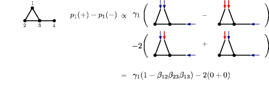
Figure 12: An example of expansion with propagation diagrams in one loop cases.

6.2 Example

Consider a graph in figure 2. In this case theorem 4 turns out to be

$$\frac{Z}{Z_{B}}p_{1}(\pm)=b_{1}(\pm)\Biggl{(}1+\beta_{23}\beta_{34}\beta_{24}\Biggr{)}+b_{1}(\mp)\beta_{14}\beta_{13}\Biggl{(}\beta_{34}+\beta_{34}\beta_{24}\beta_{23}\gamma_{3}\gamma_{4}\Biggr{)}$$

$$\mp\sqrt{b_{1}(+)b_{1}(-)}\Biggl{(}\beta_{13}\beta_{34}\beta_{23}\beta_{24}\gamma_{3}+\beta_{14}\beta_{34}\beta_{23}\beta_{24}\gamma_{4}\Biggr{)}.$$ (63)

By (63), we have

$$\frac{Z}{Z_{B}}\frac{p_{1}(+)-p_{1}(-)}{\sqrt{b_{1}(+)b_{1}(-)}}=\gamma_{1}\Biggl{(}1+\beta_{23}\beta_{34}\beta_{24}-\beta_{14}\beta_{13}\beta_{34}-\beta_{14}\beta_{13}\beta_{34}\beta_{24}\beta_{23}\gamma_{3}\gamma_{4}\Biggr{)}$$

$$-2\Biggl{(}\beta_{13}\beta_{34}\beta_{23}\beta_{24}\gamma_{3}+\beta_{14}\beta_{34}\beta_{23}\beta_{24}\gamma_{4}\Biggr{)}.$$ (64)

The right hand side discriminates which state is more plausible. Let $\beta_{34}=0$ in (64), this expression is reduced to the case of $L=1$ and consistent with the result of corollary 3. Let $\beta_{13}=0$. In this case we see that $p_{1}(+)-p_{1}(-)$ does not necessarily have the same sign as $\gamma_{1}$ [19].

If, for example, $|\beta_{ij}|\leq 1/2$, $|\gamma_{3}|,|\gamma_{4}|\leq 1$ and $|\gamma_{3}|/2,|\gamma_{2}|/2\leq|\gamma_{1}|$, then we see from (64) that $p_{1}(+)-p_{1}(-)$ and $\gamma_{1}$ have the same sign. The first condition requires weakness of the interactions, and the second condition requires that the beliefs at the nodes of degree three are not too much biased. The last condition is satisfied if $p_{1}(+)$ and $p_{1}(-)$ are not too close to each other.

If we take variables $m_{i}$ and $\tau_{ij}$ in section 5.2 instead of $\gamma_{i}$ and $\beta_{ij}$, the expressions (63) and (64) become more complicated in general, and it is hard to find simple conditions.

7 Concluding remarks

We introduced propagation diagrams that enable us to compute loop series expansion of a partition function and marginal distributions with a set of simple rules. In this method, parameters $\beta_{ij}$ and $\gamma_{i}$ are naturally assigned to each edge and node.

Accuracy of the Bethe approximation depends both on the strength of interactions and the topology of the underlying graph. The effect of the interactions is captured by the values of $\beta$ and $\gamma$. The topological aspect of the graph, in the sense of Bethe approximation, is extracted in the polynomial $\Theta$.

We suggest future research topics. First, understanding of the structure of the polynomial $\Theta$ is important to construct efficient approximation algorithms exploiting graph topology. The properties of $\Theta$ should be investigated further. Secondly, on the basis of the results of this paper, it is interesting to understand the empirically known fact: if LBP does not converge, the quality of the Bethe approximation is low [20]. Since we show a direct relation between the message passing operation and the expansion variables $\beta$ and $\gamma$, convergence of the LBP algorithm can be analyzed using them.

8 References

Appendix

A.1 Example of expansion

We consider the graph in figure 2. Normalizing $Z_{B}=1$, we can calculate the loop expansion of the partition function as in the following figure, using propagation diagrams.

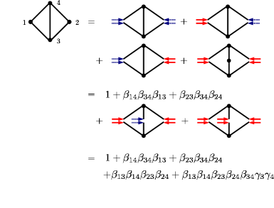
Figure 13: Expansion of the partition function with the method of propagation diagrams. It is not necessary to expand all edges as in the proof of theorem 3.

Five terms in the final expression of figure 13 correspond to the subgraphs in figure 14 respectively.

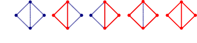
Figure 14: Light red parts are generalized loops.

References

- [1] Bethe H 1935 Proc. R. Soc.of London A 150 552–75
- [2] Murphy K, Weiss Y and Jordan M 1999 Proc. of Uncertainty in AI 467–75
- [3] Yedidia J, Freeman W and Weiss Y 2001 Adv. in Neural Information Processing Systems 13 689–95
- [4] Gallager R 1962 IEEE Trans. Inf. Theory 8 21–28
- [5] McEliece R and Cheng D 1998 IEEE J. Sel. Areas Commun. 16 140–52
- [6] Freeman W, Pasztor E and Carmichael O 2000 Int. J. Comput. Vision 40 25–47
- [7] Chertkov M and Chernyak V 2006 Phys. Rev.E 73 65102
- [8] Chertkov M and Chernyak V 2006 J. Stat. Mech: Theory Exp. 6 P06009
- [9] Pearl J 1988 Probabilistic Reasoning in Intelligent Systems: Networks of Plausible Inference (San Mateo, CA: Morgan Kaufmann Publishers)
- [10] Tatikonda S and Jordan M 2002 Uncertainty in AI 18 493–500
- [11] Yellen J and Gross J 1998 Graph Theory and Its Applications (Boca Raton: CRC Press) p 152
- [12] Baxter R 1982 Exactly Solved Models in Statistical Mechanics (London: Academic Press) p 47
- [13] Fisher M 1966 J. Math. Phys. 7 1776–81
- [14] Chertkov M, Chernyak V and Teodorescu R 2008 J. Stat. Mech: Theory Exp. 5 P05003
- [15] Chernyak V and Chertkov M 2007 Proceedings of ISIT (arXiv:cs.IT/0701086)
- [16] Domb C and Sykes M 1957 Proc. R. Soc.of London A 240 214–28
- [17] Domb C and Sykes M 1957 Philosophical Magazine 2 733–49
- [18] Sykes M 1961 J. Math. Phys. 2 52–62
- [19] Weiss Y 2000 Neural Computation 12 1–41
- [20] Mooij J and Kappen H 2005 J. Stat. Mech: Theory Exp. 11 P11012