Scale dependent galaxy bias in the SDSS as a function of
luminosity and colour

Abstract

It has been known for a long time that the clustering of galaxies changes as a function of galaxy type. This galaxy bias acts as a hindrance to the extraction of cosmological information from the galaxy power spectrum or correlation function. Theoretical arguments show that a change in the amplitude of the clustering between galaxies and mass on large-scales is unavoidable, but cosmological information can be easily extracted from the shape of the power spectrum or correlation function if this bias is independent of scale. Scale-dependent bias is generally small on large scales, $k<0.1\,h\,{\rm Mpc}^{-1}$, but on smaller scales can affect the recovery of $\Omega_{m}h$ from the measured shape of the clustering signal, and have a small effect on the Baryon Acoustic Oscillations. In this paper we investigate the transition from scale-independent to scale-dependent galaxy bias as a function of galaxy population. We use the Sloan Digital Sky Survey DR5 sample to fit various models, which attempt to parametrise the turn-off from scale-independent behaviour. For blue galaxies, we find that the strength of the turn-off is strongly dependent on galaxy luminosity, with stronger scale-dependent bias on larger scales for more luminous galaxies. For red galaxies, the scale-dependence is a weaker function of luminosity. Such trends need to be modelled in order to optimally extract the information available in future surveys, and can help with the design of such surveys.

1 Introduction

Galaxies are not expected to form a Poisson sampling of the distribution of matter in the Universe. Indeed, it has been known for some time that different populations of galaxies demonstrate different clustering strengths (Davis & Geller, 1976; Dressler, 1980; Park et al., 1994; Peacock & Dodds, 1994; Seaborne et al., 1999; Norberg et al., 2001, 2002; Zehavi et al., 2002, 2005; Li et al., 2006), showing that they cannot all have a simple relationship linking their distribution with that of the matter. This galaxy bias severely limits our ability to extract cosmological data from galaxy surveys (Percival et al., 2007; Sanchez & Cole, 2008).

The large-scale shape of the linear matter power spectrum is dependent on $\Omega_{m}h$ because of the change in the evolution of the Jeans scale after matter-radiation equality (Silk, 1968; Peebles & Yu, 1970; Sunyaev & Zel’dovich, 1970; Bond & Efstathiou, 1984, 1987; Holtzman, 1989). However, changes in the general shape of the power spectrum, such as that caused by this physical process, are hard to separate from galaxy bias, which also imprints a signature that changes smoothly with scale. Galaxy bias can also affect mode-coupling in the power spectrum by changing the non-linear scale, which can lead to small changes in the Baryon Acoustic Oscillation positions (Crocce & Scoccimarro, 2008; Matsubara, 2008). Such effects are beyond the scope of our work, and we concentrate here on the broad changes to the shape of the galaxy power spectrum.

The simplest model of galaxy bias is local, linear, deterministic bias, $\delta_{g}({\bf x})=b_{\rm lin}\delta_{\rm lin}({\bf x})$ where $\delta_{g}$ is the galaxy overdensity field, and $\delta_{\rm lin}$ is the linear mass overdensity field. In this model, the bias $b_{\rm lin}$ is constant in space, but can change for different galaxy populations. A more generic model may also include a stochastic element which enters the description as an additional term, $\delta_{g}({\bf x})=b_{\rm lin}\delta_{\rm lin}({\bf x})+\epsilon$. Or the bias could be non-local, where it depends on a smoothed version of the density field. In this paper, we will only be concerned with the relation between the galaxy and mass power spectra, and therefore define a practical measure of galaxy bias

$$P_{g}(k)=b(k)^{2}P_{\rm lin}(k).$$ (1)

Such a model can incorporate some of the complexities discussed above, but is local in $k$-space, so cannot include any mode coupling terms, which are expected to be present.

As we move to large scales, the galaxy bias is expected to tend towards a constant value. The simplest model for this is the peak-background split model (Bardeen et al., 1986; Cole & Kaiser, 1989). Here galaxy formation depends on the local density field. Large scale density modes can alter the local galaxy number density by pushing pieces of the density field above a critical threshold. On large scales we expect a linear relationship between the large scale mode amplitudes and the change in number density, so the shape of the galaxy and mass power spectra are the same. Interestingly, such a linear relationship is broken if the density field has a non-Gaussian component (Dalal et al., 2008; Slosar et al., 2008). On small scales we expect galaxy clustering to be different from that of the mass, as pairs of galaxies inside single collapsed structures become important (Seljak, 2000; Peacock & Smith, 2000; Cooray & Sheth, 2002).

Although large-scale bias is seen as a nuisance when extracting cosmological information from galaxy power spectra, it does provide constraints on possible galaxy formation models. Wild et al. (2005) proposed bivariate lognormal models of relative bias motivated by observations of galaxy distributions. The data were found to support a small (everywhere $<$5%), but significant, amount of stochasticity and non-linearity in these models on all scales, implying that galaxy formation is not solely a function of local density; these effects must be understood in order to properly utilise the next generation of galaxy surveys. A related work, Conway et al. (2005), also supported these findings.

In order to use the power spectrum to extract cosmological information, we need to investigate the transition between scale-independent and scale-dependent galaxy bias. This transition is known to be a function of the galaxy population chosen. Comparing work in Cole et al. (2005) and Percival et al. (2007), which used the same techniques, and the analysis of Sanchez & Cole (2008), shows that there are deviations between the shapes of the 2dFGRS and SDSS galaxy power spectra. If this results from galaxy bias and the fact that the 2dFGRS selected galaxies in a blue band whilst the SDSS selected galaxies in a red band, then we should expect that similar changes show up in red and blue galaxies drawn from a single survey. Using the SDSS, Percival et al. (2007) showed that at $k=0.2\,h\,{\rm Mpc}^{-1}$, the shape of the power spectrum is a strong function of the $r$-band luminosity. In this paper we extend this work by splitting in galaxy colour and luminosity, and by fitting models to the resulting power spectra, in order to see if the SDSS contains sufficient galaxies to fully explain the trend observed between SDSS and 2dFGRS galaxies.

Previous work examining the observed dependence of the large scale bias on luminosity was carried out by Norberg et al. (2001) who proposed the phenomenological model $b=b_{1}+b_{2}L/L_{\star}$, Tegmark et al. (2004) extended this to better fit the available data by including an extra parameter in the form $b=b_{1}+b_{2}L/L_{\star}+b_{3}(M-M_{\star})$. Swanson et al. (2008) reexamined both these models for samples split by galaxy colour. Wild et al. (2005) also examined the colour dependence of relative bias. Zehavi et al. (2005) presented colour dependent and luminosity dependent measurements of the projected correlation function of SDSS galaxies. In all cases subsets of the data existed where some aspect of the bias model in question was shown to be a function of colour or luminosity.

We first describe the SDSS catalogues we use in Section 2, and how we model the radial selection function of our subsamples using luminosity function fits in Section 3. Section 4 describes our calculation of power spectra and uncertainties, and the bias models to be fitted are presented in Section 5. Results of fitting the bias models are given in Section 6. In Section 7 we present simple models for the luminosity dependence of our bias parameters and the results of fitting these to our data. Conclusions and discussion are presented in Section 8.

2 Galaxy Catalogues

We use galaxy catalogues selected from the Sloan Digital Sky Survey DR5 main galaxy sample. The Sloan Digital Sky Survey (SDSS; York et al. 2000; Adelman-McCarthy et al. 2006), which was recently completed, used a 2.5m telescope (Gunn et al., 2006) to obtain $10^{4}$ square degrees of imaging data in five passbands $u$, $g$, $r$, $i$ and $z$ (Fukugita et al., 1996; Gunn et al., 1998). The main galaxy sample (Strauss et al., 2002) consists of galaxies with Petrosian $r$-band magnitude $m_{r,petrosian}\leq 17.77$. This gives approximately $90$ galaxies per square degree, with a median redshift $z=0.11$; in this paper we use the DR5 sample (Adelman-McCarthy et al., 2006). We exclude a small subset of the data taken during initial survey operation, for which the apparent magnitude limit fluctuated. This gives $410\,095$ galaxies with $14.5\leq m_{r,petrosian}\leq 17.77$ and redshift $>0.003$; the lower redshift cut strongly reduces the contribution from mis-classified stars. This is the catalogue used in Percival et al. (2007), and further details can be found here.

Where specified, we have K-corrected the galaxy luminosities using the methodology outlined in Blanton et al. (2003a, b). We also use the same $z=0.1$ shifted $r$-band filter to define our luminosities (as discussed in Blanton et al. 2003b), which we refer to as M${}_{{}^{0.1}r}$ throughout this paper. Absolute magnitudes and $k$-corrections were calculated assuming $h=100\,{\rm kms}^{-1}{\rm Mpc}^{-1}$, $\Omega_{M}=0.3$ and $\Omega_{\Lambda}=0.7$, and we have applied the recommended AB corrections to the observed SDSS magnitude system (Smith et al., 2002).

bin	absolute	mean	galaxy
	magnitude	$M_{0.1_{r}}$	count
	range
red 1	-22.30 ${\leq}$ $\,M_{0.1_{r}}<$ -21.35	$-21.79\pm 0.27$	49167
red 2	-21.35 ${\leq}$ $\,M_{0.1_{r}}<$ -20.89	$-21.12\pm 0.13$	41462
red 3	-20.89 ${\leq}$ $\,M_{0.1_{r}}<$ -20.47	$-20.70\pm 0.12$	37819
red 4	-20.47 ${\leq}$ $\,M_{0.1_{r}}<$ -20.00	$-20.27\pm 0.14$	34651
red 5	-20.00 ${\leq}$  $M_{0.1_{r}}<$ -19.34	$-19.75\pm 0.19$	29742
red 6	-19.34 ${\leq}$ $\,M_{0.1_{r}}<$ -17.00	$-19.01\pm 0.38$	17582
blue 1	-22.30 ${\leq}$ $\,M_{0.1_{r}}<$ -21.35	$-21.67\pm 0.24$	17480
blue 2	-21.35 ${\leq}$ $\,M_{0.1_{r}}<$ -20.89	$-21.22\pm 0.13$	25208
blue 3	-20.89 ${\leq}$ $\,M_{0.1_{r}}<$ -20.47	$-20.69\pm 0.12$	28928
blue 4	-20.47 ${\leq}$ $\,M_{0.1_{r}}<$ -20.00	$-20.27\pm 0.14$	32066
blue 5	-20.00 ${\leq}$  $M_{0.1_{r}}<$ -19.34	$-19.74\pm 0.19$	36889
blue 6	-19.34 ${\leq}$ $\,M_{0.1_{r}}<$ -17.00	$-18.91\pm 0.49$	48754

Table 1: Description of the subcatalogues analysed in this paper. The limits of the absolute magnitude bins are given, with the weighted mean and standard deviation. We also give the galaxy count for each bin.

Figure 1: The distribution of galaxies in colour-absolute magnitude space. The dashed line denotes the boundary of the colour split at $M_{0.1_{g}}-M_{0.1_{r}}=0.8$.

Figure 2: The distribution of galaxies in absolute magnitude–redshift space, red galaxies are shown in the top panel, blue galaxies in the lower panel. The horizontal, dashed lines denote the boundaries of the absolute magnitude bins.

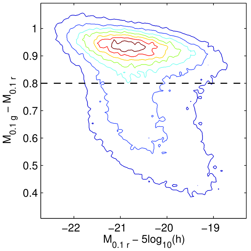
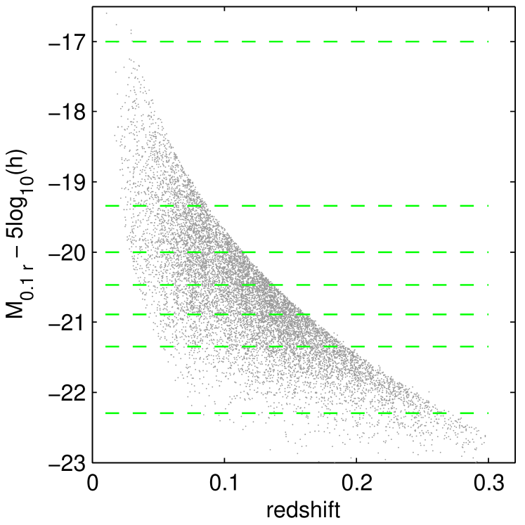
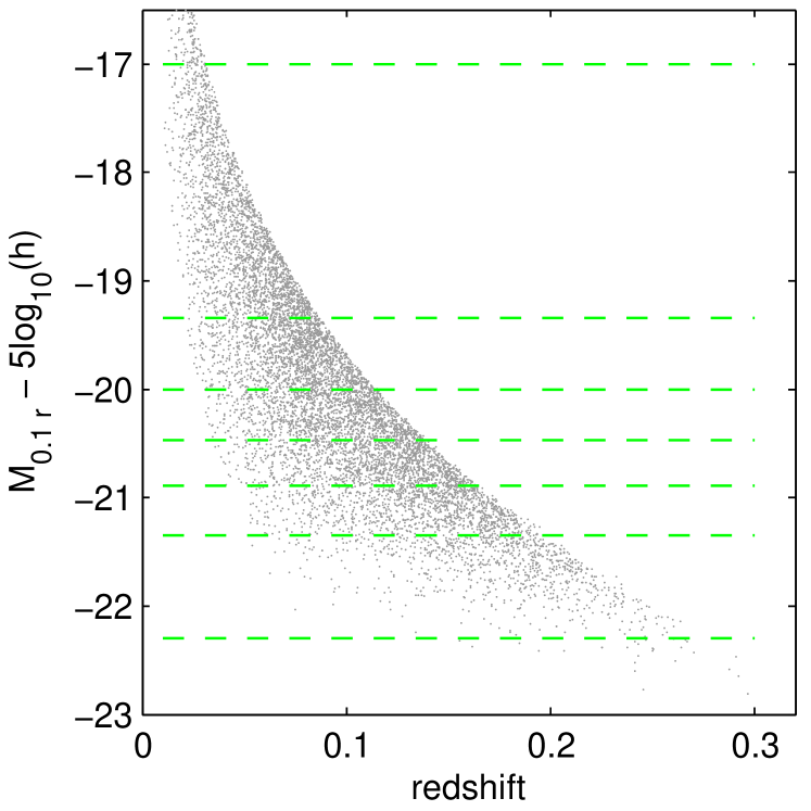
This sample of main galaxies was split into 6 absolute magnitude limited subsamples giving approximately equal numbers of galaxies in each bin. Each subsample was then further divided into red and blue subsamples defined by a constant colour cut of $M_{0.1_{g}}-M_{0.1_{r}}=0.8$. Fig. 1 illustrates our chosen simple colour split, showing that this cut clearly divides the two populations. We have tried more complicated cuts without significant change in our results.

The absolute magnitude cuts and number of galaxies in each of these subcatalogues is given in Table 1. Fig. 2 illustrates the distribution of red and blue galaxies within the imposed absolute magnitude limits. At a given absolute magnitude the high and low redshift limits result from the apparent magnitude limits of the survey, this can be seen in Fig. 2. We could have cut the catalogues in order to make these sub-catalogues volume limited, but we wish to retain as much signal as possible. Significant cuts would have been required in order to remove all effects of evolution and K-corrections. Percival et al. (2007) showed a compromise using “pseudo-volume limited” catalogues. We choose instead to estimate the redshift distribution by fitting the luminosity function (see the next section), so we can model an apparent magnitude cut as easily as a cut in absolute magnitude. This approach allows us to work with considerably more galaxies and retain the maximum information.

3 Modelling the Radial Selection Functions

For each of the catalogues described in the previous section, we need to model the radial selection function. The angular mask is the same for all catalogues as all the cuts being applied are independent of angular position. We use a HEALPIX (Górski et al., 2005) mask to describe the angular galaxy distribution as described in Percival et al. (2007). We derive the radial distribution of galaxies in each of our samples from fits to the luminosity functions for either red or blue galaxies as appropriate. Section 3.1 describes our luminosity function model and Section 3.2 describes our method for transforming this into a redshift distribution.

3.1 Redshift evolution corrected luminosity functions

Our subsamples of red and blue galaxies contain sufficiently large numbers of galaxies to allow us to calculate redshift evolution corrected luminosity functions. We have found that well known Schechter function (Schechter, 1976) fits the data well. In terms of absolute magnitude and with modifications to include redshift evolution the Schechter function is given by

$$\Phi(M,z)\,dM\,dV=\bar{n}\,0.4\log_{e}(10)\,10\,^{\,0.4\,(z-z\,_{0})\,P}\\ 10\,^{\,0.4\,(M^{\star}-M-Q\,(z-z\,_{0})\,)\,(1+\alpha)}\,exp\,{\{-10^{\,0.4\,(M^{\star}-M-Q\,(z-z\,_{0})\,)}\}}\,dM\,dV,$$ (2)

where $P$ and $Q$ are redshift evolution parameters following the convention of Lin et al. (1999): $P$ allows for density evolution, while $Q$ allows for luminosity evolution. We have also tried fitting non-parametric models, models with so many parameters that the final shape of the function is to an extent independent of the shapes of the contributing terms, based on the work of Blanton et al. (2003b). However we find no significant change in the resulting redshift distribution, and we therefore only consider fitting a Schechter function in the remainder of our paper.

Figure 3: The best fit redshift-evolution corrected Schechter functions (Eq.2, see text for details) representing the luminosity functions of the red galaxies, shown as the solid red line, and blue galaxies, shown as the dashed blue line, both at a redshift of $z=0.1$. The red, vertical crosses and blue, diagonal crosses represent the $1/V_{max}$ data estimates of the true luminosity function for red and blue galaxies respectively, redshift evolution corrected using the respective best fit parameters for Eq. 2 to a redshift of $z=0.1$.

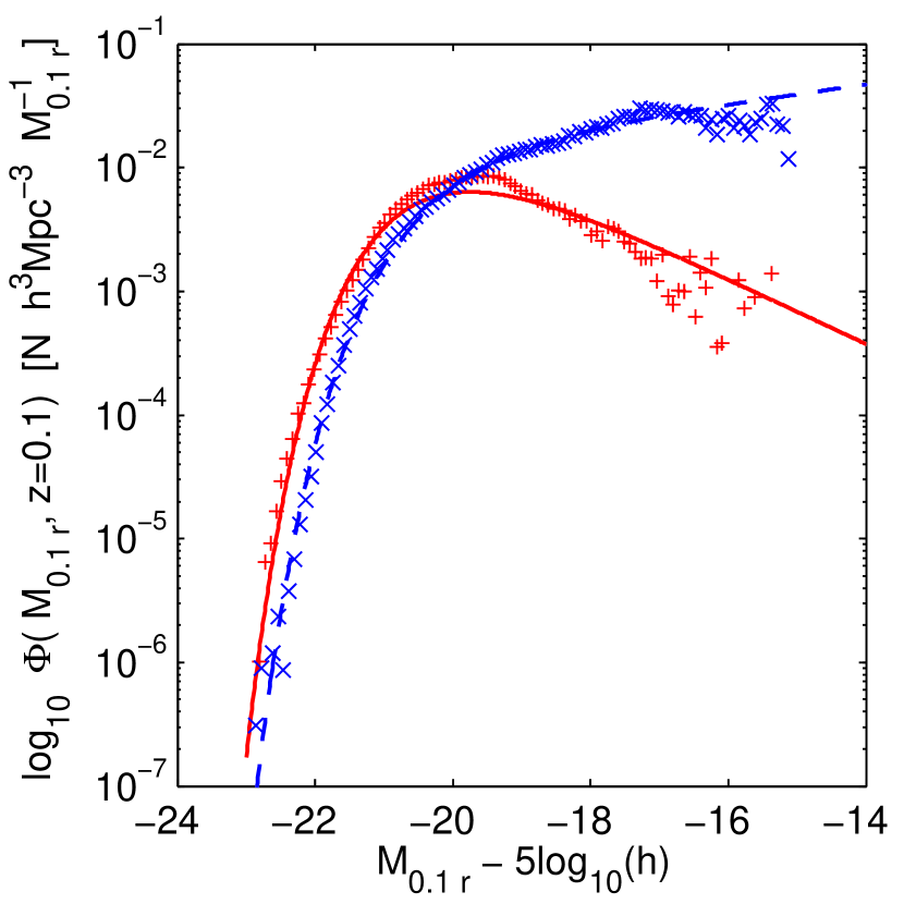
The luminosity function parameters were determined using a maximum likelihood method (Lin et al., 1999) implemented with the minimisation routine Powell (Press et al., 1992). Convergence to the Likelihood maximum was confirmed by starting the minimisation routine at a number of widely separated initial parameter sets, and observing that the same best-fit parameters were obtained. The results for the red and blue galaxy samples can be seen in Fig. 3. Note that the overall normalisation, $\bar{n}$ cannot be determined by this maximum likelihood method and we determine it directly from the data. Further discussion of our procedure to calculate luminosity functions and the parameters of the resulting fits will be presented in Cresswell et al. (2008). In this paper we simply use the luminosity functions to estimate redshift distributions for the selected catalogues, so the recovered parameters are not important, provided the fits are an adequate match to the data: for instance, there is some apparent discrepancy between the $1/V_{max}$ data estimates and the best fit Schechter function for the red galaxies near an absolute magnitude of $M_{0.1_{r}}\approx-19.3$; as the luminosity function is slowly changing in this region and the normalisation is determined independently of the fit this will have no significant effect on the shape of any derived redshift distributions, which would here be dominated by the effect of the apparent magnitude limits of the survey.

3.2 Redshift distributions

Figure 4: Histogram showing the redshift distribution of red galaxies in absolute magnitude bin 2. The thick black line is the model distribution derived from the red galaxy luminosity function via the relation shown in Eq. (3).

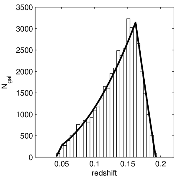
Given a luminosity function as defined in Eq. (2) we can integrate to determine the redshift distribution using

$$f(z)\,dz\propto\int_{M_{\rm lower}}^{M_{\rm upper}}\Phi(M^{\prime},z)dM^{\prime}\frac{dV}{dz}dz,$$ (3)

where $M_{\rm lower}$ is the minimum of the lower survey absolute magnitude limit at a given redshift, and the lower bin magnitude limit, and $M_{\rm upper}$ is similarly defined from the upper boundaries of the sample and bin. An example of the data and model redshift distributions for one of the subsamples, the red galaxies in absolute magnitude bin 3, is shown in Fig. 4. Good agreement is seen in this plot, and between model and data redshift distribution for all of our subsamples, validating our procedure.

4 calculating power spectra and uncertainties

Power spectra were calculated as described in Percival et al. (2007), using the standard Fourier technique of Feldman et al. (1994). The radial and angular selection functions were included in this method by creating a random catalogue with the same selection function as the galaxies, but with Poisson sampling and 10$\times$ as many galaxies. The galaxies were weighted using the optimal weights of Feldman et al. (1994). Obviously, no additional bias-dependent weighting scheme (such as that in Percival et al. 2004 was applied).

For the SDSS DR5 sample we have created 2000 Log-Normal (LN) catalogues, calculated as described in Cole et al. (2005). We assumed a flat $\Lambda$CDM power spectrum with $\Omega_{m}h=0.2$, and $\Omega_{b}/\Omega_{m}=0.15$. Normalisation was matched to that of $L_{*}$ galaxies as defined below. We have applied a colour and luminosity dependent bias model that is scale-independent to these catalogues. The scheme was iteratively matched to our results: initially we used the luminosity-bias relation of Norberg et al. (2001) to calculate catalogues and the corresponding covariance matrix for the data. Having fitted the data, we then calculated new catalogues with a colour-luminosity bias scheme that was a better fit to the data. This change resulted in a negligible change to the best-fit bias model, so we are confident that our results do not depend on this choice.

Power spectra were calculated from the mock catalogues using exactly the same process as for the actual data, and the covariance matrices were estimated for each of the subcatalogues described in Section 2. Because LN catalogues for each subcatalogue were drawn from the same underlying density fields, we use these mocks to calculate correlations between the power spectra for different subcatalogues: these will be correlated as the volumes overlap.

5 Fitting Models of Galaxy Bias

As discussed in Section 1, we define bias as the ratio between the galaxy power spectra and the linear matter power spectrum (Eq. 1). We fit the observed power spectra with models calculated from a linear model power spectra, using the fitting formulae of Eisenstein & Hu (1998), with parameters given by the concordance cosmology $\Omega_{0}=0.241$, $\Omega_{\Lambda}=0.759$, $H_{0}=73.2$, $\sigma_{8}=0.761$, $n_{s}=0.958$, $\Omega_{b}/\Omega_{m}=0.175$ (Spergel et al., 2006), multiplied by a bias model. The model is then convolved with the window function for each catalogue, as described in Percival et al. (2007). We will be interested in relatively large scales $k<0.4\,h\,{\rm Mpc}^{-1}$ and assume that, on these scales, the power spectrum band-powers result from a multi-variate Gaussian distribution, and that they are correlated within a single power spectrum, and between different power spectra. We perform Maximum Likelihood fits to the measured power spectra for three models of the bias $b(k)$. First we assume that the bias is constant and fit on scales $k<0.21\,h\,{\rm Mpc}^{-1}$. We then consider two scale-dependent models for $b(k)$, fitting to smaller scales. Results are given in section 6.

First we use the $Q$-model (Cole et al., 2005),

$$b(k)=b_{\rm lin}\sqrt{\frac{1+Qk^{2}}{1+Ak}},$$ (4)

where $b_{\rm lin}$ is the asymptotic large-scale bias, and $Q$ and $A$ are parameters. Cole et al. (2005) used halo model catalogues to suggest that $A=1.4$ in redshift-space leaving just a single nuisance parameter $Q$ to be fitted to data. $Q$ would be expected to change for different galaxy populations, and it is this that we test as a function of galaxy colour and luminosity.

We also consider a model with

$$b(k)=b_{\rm lin}\sqrt{1+\frac{P}{b_{\rm lin}^{2}P_{\rm lin}}},$$ (5)

where the parameter $P$ acts as an additional shot noise term. This model has a physical basis as this term could account for a change in the shot noise. This would arise if halos Poisson sampling the density field, and galaxies are located in those halos, i.e. $P$ is the contribution to the galaxy power spectrum from the one-halo term Seljak (2001); Schulz & White (2006); Guzik et al. (2007). We will refer to this model as the $P$-model.

The relative merits of these two models are discussed in Smith et al. (2006), who argue in favour of the ease of physical interpretation of the $P$-model. In addition, although they show that for classes of cosmological model containing a free-streaming hot dark matter component consisting of relic thermal axions, the $Q$-model becomes highly pathological due to a degeneracy between $Q$ and the particle mass. They suggest that this pathology may extend to other models with light thermal relic components.

6 Results from fitting the power spectra

Figure 5: Comparison of relative, large-scale, constant, linear bias as a function of luminosity for galaxies split into red and blue colours. Five and six pointed stars represent our measurements of bias relative to our red galaxy $M_{\star}$ bin, for red and blue galaxies respectively. Squares and circles show the results from Swanson et al. (2008) renormalised to match our $M_{\star}$ values, see text for details. The upper, solid line is a fit to Eq. 6 for our red galaxy bias points, see text for details. The lower, dash-dot line is the fit to blue galaxies. The horizontal dashed line shows no bias relative to our red $M_{\star}$ bin.

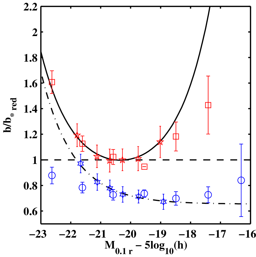
We have fitted bias models to power spectra calculated from the catalogues parametrised in Table 1. First we consider fitting scale-independent bias on large scales, and then we consider scale-dependent bias. All bias measurements were calculated relative to the bias of red galaxies of luminosity $L_{\star}$, $b_{\star,{\rm red}}$, where $L_{\star}$ was calculated from the fit to the red-galaxy luminosity function.

6.1 Large scale bias

If we assume that the bias does not change with scale, and fit to very large scales $k<0.21\,h\,{\rm Mpc}^{-1}$, then the resulting bias amplitudes, measured relative to $b_{\star,{\rm red}}$, are shown in Fig. 5. For comparison we also plot the data of Swanson et al. (2008) with an average evolution correction removed from each magnitude bin. In order to compare samples with different $L_{\star}$ values the Swanson et al. (2008) data have been offset to so that the linear interpolation of the data points either side of our $L_{\star}$ bin passes through our $L_{\star}$ bin, these corrections are small, $\approx-0.05$ M${}_{{}^{0.1}r}$ for red galaxies and $\approx+0.01$ M${}_{{}^{0.1}r}$ for blue galaxies. As can be seen, we recover the same trends with the bias of blue galaxies monotonically increasing with galaxy luminosity, while the red galaxies show more complicated behaviour with increased bias for both high and low luminosity galaxies. This comparison is discussed further in Section 8.

6.2 Scale dependent bias

The best-fit parameters for the $Q$-model and $P$-model fits are presented in Table 2. These numbers were calculated by fitting each of the 12 power spectra with the bias model multiplied by the linear power spectrum. The best-fit values and their trends as a function of galaxy colour and luminosity are analysed further in Section 7.

	$Q$-model		$P$-model
bin	$b_{lin}$	$Q$	$b_{lin}$	$P$
red 1	$1.40\pm 0.02$	$9.45\pm 0.70$	$1.35\pm 0.02$	$512\pm 48$
red 2	$1.22\pm 0.03$	$9.24\pm 0.83$	$1.17\pm 0.03$	$375\pm 40$
red 3	$1.17\pm 0.03$	$9.44\pm 0.94$	$1.13\pm 0.03$	$351\pm 42$
red 4	$1.20\pm 0.04$	$7.72\pm 0.93$	$1.16\pm 0.04$	$277\pm 46$
red 5	$1.25\pm 0.05$	$7.26\pm 1.03$	$1.20\pm 0.05$	$272\pm 51$
red 6	$1.44\pm 0.08$	$8.03\pm 1.45$	$1.39\pm 0.07$	$419\pm 80$
blue 1	$1.09\pm 0.03$	$13.74\pm 1.29$	$1.04\pm 0.03$	$541\pm 48$
blue 2	$0.96\pm 0.03$	$9.89\pm 1.34$	$0.92\pm 0.03$	$274\pm 40$
blue 3	$0.94\pm 0.04$	$7.74\pm 1.43$	$0.90\pm 0.04$	$177\pm 43$
blue 4	$0.89\pm 0.05$	$7.44\pm 1.74$	$0.86\pm 0.05$	$151\pm 46$
blue 5	$0.91\pm 0.07$	$4.64\pm 1.78$	$0.87\pm 0.06$	$66\pm 51$
blue 6	$0.92\pm 0.14$	$2.99\pm 2.97$	$0.87\pm 0.13$	$17\pm 80$

Table 2: Maximum Likelihood parameters calculated by fitting the $Q$-model and $P$-model for scale-dependent galaxy bias as given in Eqns. 4 & 5, to power spectra calculated for the catalogues described in Section 2. Best-fit values are presented together with 1-$\sigma$ uncertainties.

Figure 6: Comparison of best-fit power spectra calculated with bias from the $Q$-model (solid lines) to the data (circles with 1$\sigma$ errors). Each power spectrum is divided by our fiducial linear power spectrum convolved with the appropriate window function.

Figure 7: As Fig. 6, but now for model power spectra calculated assuming the $P$-model for galaxy bias.

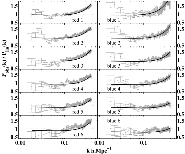
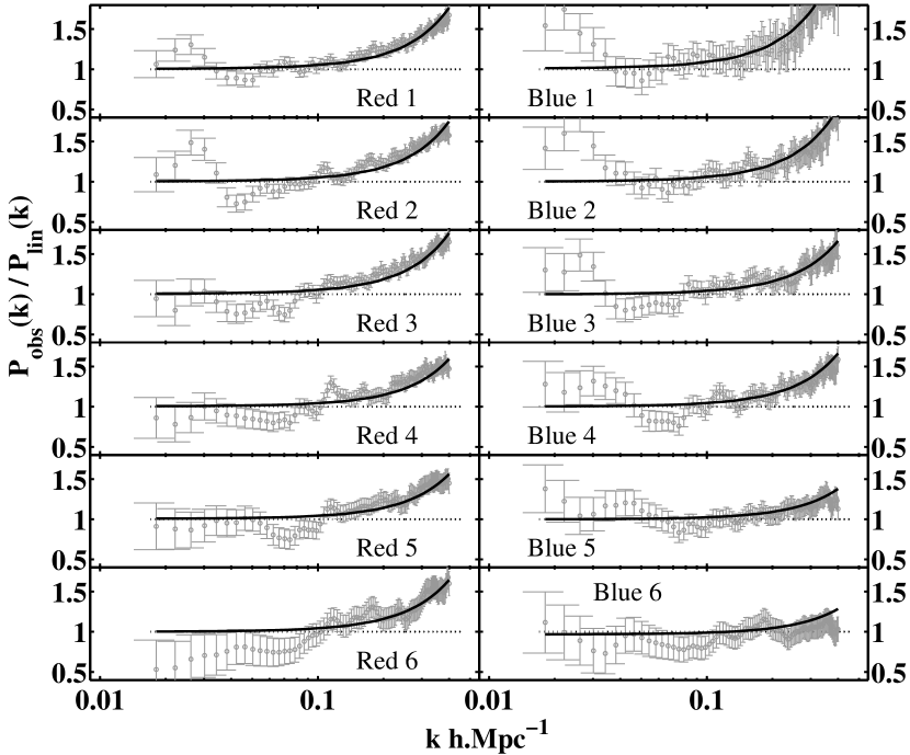
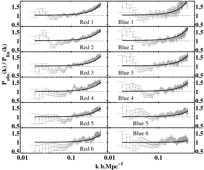
The model and data power spectra are compared in Figs. 6 & 7. These data are divided by our fiducial model convolved with the appropriate window function. Comparisons are shown for the red galaxies in the left hand panels and blue galaxies on the right, with the rows of panels showing different absolute magnitude bins with the brightest at the top and faintest at the bottom. The offset visible between the data and model in the lower left panel is due to the high best-fit large-scale bias in the best-fit solution (Eq. 6, fit parameters given in Table 2). Such effects arise because the data are correlated, and the maximum Likelihood solution does not match the $\chi$-by-eye expectation.

7 Modelling bias as a function of luminosity

Figure 8: Top row: best-fit $b_{lin}$, and $Q$ model parameters as a function of absolute magnitude, as presented in Table 2, from a fit including the $Q$-model bias prescription. Bottom row: best-fit $b_{lin}$, and $P$ model parameters as a function of absolute magnitude, as presented in Table 2, from a fit including the $P$-model bias prescription. Circles and crosses are for red and blue galaxies respectively. Solid, horizontal lines about each data point show the extent of each absolute magnitude bin. Solid lines show the models of Eqns. 9 & 11 and dashed lines show the models of  10 & 12 in the appropriate panels for red and blue galaxies respectively.

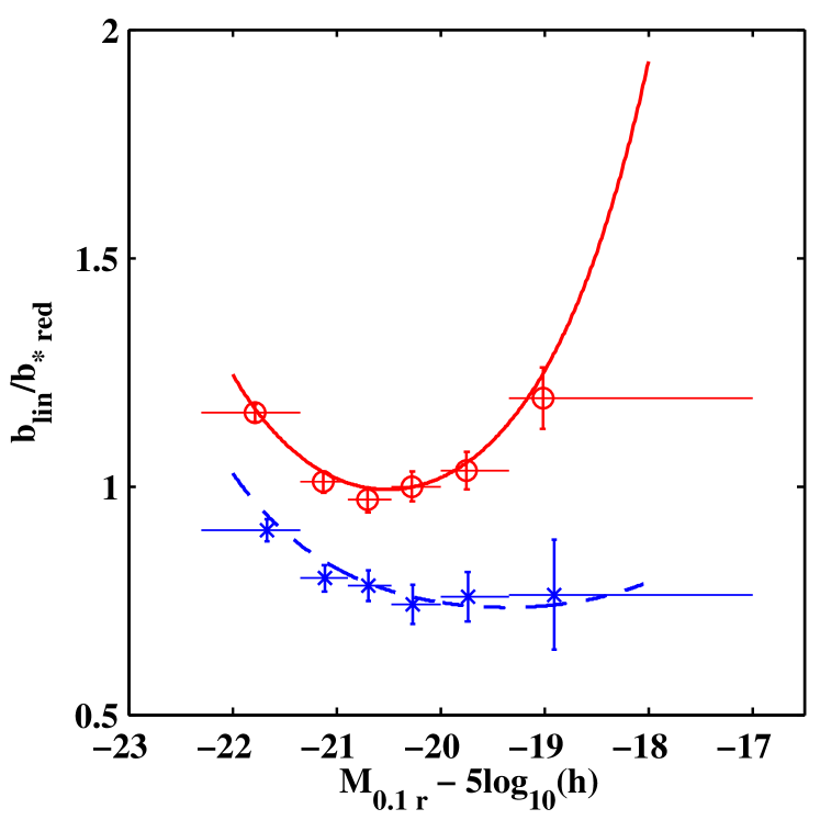
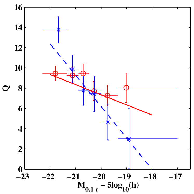
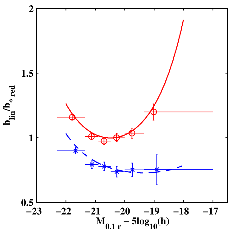
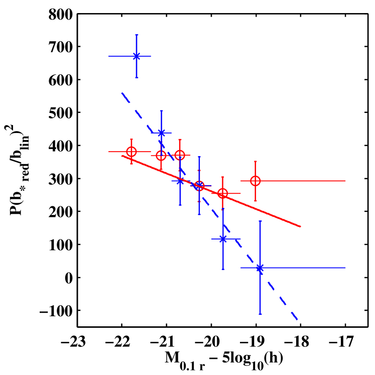
In this section we try to fit a simple model for the luminosity dependence of the parameters in the bias models given in Eqns. 4 & 5.

The asymptotic large-scale bias $b_{\rm lin}$ is known to be a function of galaxy luminosity (Norberg et al., 2001; Tegmark et al., 2004), and galaxy colour (Swanson et al., 2008). Here, we extend the form of the model introduced by Norberg et al. (2001) in order to cope with the more complicated behaviour seen when we also split galaxies by colour. We assume the three parameter model

$$b_{\rm lin}(L)=a_{1}+a_{2}\frac{L}{L_{\star}}+a_{3}\frac{L_{\star}}{L}.$$ (6)

For relative biases where $b_{\rm lin}(L_{\star})=1$, we would have that $a_{1}+a_{2}+a_{3}=1$, so the model would only have two free parameters. This model reduces to the form of Norberg et al. (2001) in the case of $a_{3}=0$.

In addition, we parametrise

$$Q(L)=q_{1}+q_{2}(M-M_{\star}),$$ (7)

and

$$P(L)=p_{1}+p_{2}(M-M_{\star}),$$ (8)

where $q_{1}$, $q_{2}$, $p_{1}$ and $p_{2}$ are parameters that we can fit to the data. We therefore have 5 free parameters in our fit to the data in addition to choice of whether to use the P or $Q$-model. We have fitted these parameters by performing a simultaneous Maximum Likelihood search using all 12 power spectra, and allowing for covariances between band powers in each, and between different power spectra. I.e. we do not simply fit the recovered data values in Fig. 8, but instead perform a new fit to the data. The resulting bias models are compared with the results calculated when we allowed $b_{\rm lin}$, $Q$ and $P$ to match each catalogue individually in Fig. 8. As can be seen, this simple model does very well in matching the luminosity-dependent trends observed.

Figure 9: As Fig. 6, but now showing models with parameters calculated from a simple fit to the luminosity dependent trends observed in Fig. 8.

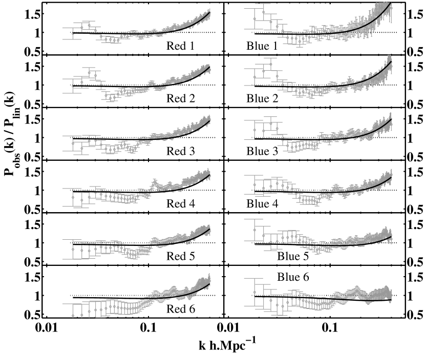
The resulting best-fit parameters allow us to define the following models for redshift-space galaxy power spectra. Using the $Q$-model, for red galaxies,

$$P_{gal\,red}(L,k)=\left(0.92+0.10\frac{L}{L_{\star}}+0.19\frac{L_{\star}}{L}\right)^{2}\\ \times P_{\rm lin}(L,k)\left(\frac{1+(7.5-1.0(M-M_{\star}))k^{2}}{1+Ak}\right),$$ (9)

and for blue galaxies,

$$P_{gal\,blue}(L,k)=\left(0.81+0.07\frac{L}{L_{\star}}+0.02\frac{L_{\star}}{L}\right)^{2}\\ \times P_{\rm lin}(L,k)\left(\frac{1+(6.3-3.1(M-M_{\star}))k^{2}}{1+Ak}\right).$$ (10)

These model power spectra are compared with those observed in Fig. 9, where good agreement is seen.

Figure 10: As Fig. 7, but now showing models with parameters calculated from our simple fit to the luminosity dependent trends observed in Fig. 8.

Using the $P$-model, for red galaxies,

$$P_{gal\,red}(L,k)=\left(0.89+0.10\frac{L}{L_{\star}}+0.18\frac{L_{\star}}{L}\right)^{2}\\ \times{P_{\rm lin}(L,k)+\left(200-40(M-M_{\star})\right)},$$ (11)

and for blue galaxies,

$$P_{gal\,blue}(L,k)=\left(0.77+0.07\frac{L}{L_{\star}}+0.02\frac{L_{\star}}{L}\right)^{2}\\ \times{P_{\rm lin}(L,k)+\left(160-130(M-M_{\star})\right)},$$ (12)

where, as previously noted in the text, $A=1.4$. These model power spectra are compared with those observed in Fig. 10 where, as in Fig. 9, good agreement is seen.

The $\chi^{2}$ values of the best-fit models including the $P$-model of bias are good, with $609$ given $571$ degrees-of-freedom for the red galaxies and $439$ for the blue galaxies given the same number of degrees of freedom for the blue galaxies. For the $Q$-model, the corresponding numbers are $624$, and $440$. These numbers depend strongly on the covariance model adopted and, as a consequence, we do not analyse these further other than to note that the fits seem to give reasonable numbers.

8 Conclusions

We have quantified the bias of red and blue galaxies as a function of luminosity on scales $k<0.4\,h\,{\rm Mpc}^{-1}$. We find clear differences in the large-scale asymptotic bias between blue and red galaxies, similar to that found by Zehavi et al. (2005) and Swanson et al. (2008), and shown in Fig. 8. At large scales red galaxies have are more biased than blue galaxies for all luminosities. The bias of blue galaxies is a strong, monotonically increasing function of luminosity, with more luminous galaxies being the most biased. For red galaxies, the picture is more complicated, with an increase in the bias of faint red galaxies (Zehavi et al. (2005) find a similar result but stress the scale dependence of the observation). This trend is significant at the $7.2-\sigma$ level.We find a stronger bias for luminous blue galaxies, compared with that of Swanson et al. (2008). The reason for this is unknown, although it is worth noting that our catalogue is larger than that used by Swanson et al. (2008), as they used additional cuts, constructing volume limited subsamples, compared with our sample selection procedure (see section 2). We performed a simple test of the dependence of this difference on observed scale, repeating our analysis for scales $0.038<k<0.070\,h\,{\rm Mpc}^{-1}$ which approximates the Swanson et al. (2008) measurement scale of $\sim 20\,h^{-1}\,{\rm Mpc}$, the discrepancy in the bias of the brightest blue galaxies was not removed. However, the change of scales brought the best fit red galaxy linear bias model into better agreement with the Swanson et al. (2008) faint, red galaxies; the model is poorly constrained at the faint end due to the lack of unique data points in that range. It is worth noting that, due to different colour cut criteria, the brightest absolute magnitude bins in Swanson et al. (2008) are inherently more red than ours, this might lead one to expect larger bias measurements for those bins, the opposite of the observed trend. The bright blue sample contains the smallest numbers of galaxies, so the errors on the relative bias should be the largest of any sample. However, our expected errors are insufficient to fully explain the discrepancy, and there remains no obvious reason for this difference.

The work on constant bias models has been extended by considering how the turn-off from constant large-scale bias depends on galaxy colour and luminosity. We have compared two models for this turn-off: the $P$-model and $Q$-model given in Eqns. 4 & 5 respectively. We find that there is little to choose between the two in terms of how well they can fit the current data, and both provide adequate fits to the power spectrum trends observed as a function of galaxy luminosity and colour at the current level of data precision. Although there is no observational motivation, Hamann et al. (2008) argued that the $P$-model has a physical motivation, and therefore offers a more attractive model of bias.

We use the values of $P$ and $Q$ obtained for these two models to quantify the degree of divergence from a constant bias model. Note that these parameters change both the position and amplitude of the turn-off. We find that the best-fit values of $P$ and $Q$, shown in Fig. 8, are a strong function of luminosity for blue galaxies. Red galaxies show far weaker evolution with luminosity, and are consistent with the hypothesis of no change in the scale at which the bias can no longer be described as a constant, to current data precision. Interestingly, this trend in the turn-off from apparent scale-independent behaviour does not match that of the amplitude of the large-scale bias. If amplitude and turn-off scale were linked, we might have expected the $Q$ and $P$ parameters to match for red galaxies of high or low luminosity, where the constant bias component matches, but be different for intermediate luminosity galaxies. We do not observe such a trend, suggesting that there might not be a simple link between the amplitude of bias and the scale at which the 1-halo term becomes important.

It is clear that the simple $P$ and $Q$-models will become insufficient to model the observational data, both on very small scales, and as the data improve. They are, after all, simply motivated to fit observed trends, and do not encompass all of the physics involved. One alternative and more complex prescription for bias prediction is that presented in Yoo et al. (2008) which can predict $P_{obs}(k)$ given a set of cosmological parameters and a HOD model, the parameters of which have been determined from the observed, projected correlation function (the correlation function provides additional information to that of the power spectrum as they are sensitive to different scales). However, the potential limits of simple, phenomenological models, such as the $P$ and $Q$-models, does not stop us being able to use them to investigate trends in the data, as we have done in this paper. The current data clearly show that, on relatively large scales (our small scale limit of $0.4\,h\,{\rm Mpc}^{-1}$ approximately corresponds to $17\,h^{-1}\,{\rm Mpc}$), blue and red galaxies have very different bias properties. It is the blue galaxies that are faint in the $r$-band whose relative clustering on different scales most closely resembles that of the mass, and the luminous blue galaxies the least. This supports the hypothesis that the shapes of the 2dFGRS and SDSS main galaxy power spectra of Cole et al. (2005) and Tegmark et al. (2004); Percival et al. (2007) differ because the average galaxy bias of each sample differs, caused by different sample selections. The clustering of the 2dFGRS galaxies, on average, would be expected to be a better tracer of the linear clustering signal out to smaller scales than the SDSS galaxies.

This highlights the importance of sample selection for future galaxy surveys, and the importance of understanding galaxy bias for extracting cosmological information from power spectrum shapes from such surveys. Red and blue galaxies show very different trends in their large-scale bias and the scale-dependent smaller-scale bias as a function of luminosity. It is clear that galaxies need to be split into sub-populations by more than just the luminosity in a single band in order to properly understand and model bias.

References

- Adelman-McCarthy et al. (2006) Adelman-McCarthy J., et al., 2006, ApJ Suppl., 162, 38
- Bardeen et al. (1986) Bardeen J.M., Bond J.R., Kaiser N., Szalay A.S., 1986, ApJ, 304, 15
- Blanton et al. (2003a) Blanton M.R., Lin H., Lupton R.H., Maley F.M., Young N., Zehavi I., Loveday J., 2003a, Astron. J., 125, 2276
- Blanton et al. (2003b) Blanton M.R., et al., 2003b, ApJ, 592, 819
- Bond & Efstathiou (1984) Bond, J.R. & Efstathiou, G. 1984, ApJ, 285, L45
- Bond & Efstathiou (1987) Bond, J.R., & Efstathiou, G., 1987, MNRAS, 226, 655
- Cole & Kaiser (1989) Cole S., Kaiser N., 1989, MNRAS, 237, 1127
- Cole et al. (2005) Cole S., et al., 2005, MNRAS, 362, 505
- Conway et al. (2005) Conway E., et al., 2005, MNRAS, 356, 456
- Cooray & Sheth (2002) Cooray A., Sheth R., 2002, Physics Reports, 372, 1
- Cresswell et al. (2008) Cresswell J.G., et al., 2008, in preparation
- Crocce & Scoccimarro (2008) Crocce M., Scoccimarro R., 2008, PRD77, 023533
- Dalal et al. (2008) Dalal N., Olivier D., Huterer D., Shirokov A., 2008, PRD77, 123514
- Davis & Geller (1976) Davis M., Geller M.J., 1976, ApJ, 208, 13
- Dressler (1980) Dressler A., 1980, ApJ, 236, 351
- Eisenstein & Hu (1998) Eisenstein D.J., Hu W., 1998, ApJ, 496, 605
- Feldman et al. (1994) Feldman H.A., Kaiser N., Peacock J.A., 1994, MNRAS, 426, 23
- Fukugita et al. (1996) Fukugita M., Ichikawa T., Gunn J.E., Doi M., Shimasaku K., Schneider D.P., 1996, Astron. J., 111, 1748
- Górski et al. (2005) Górski, K.M., Hivon E., Banday A.J., Wandelt B.D., Hansen F.K., Reinecke M., Bartelmann M., 2005, ApJ, 622, 759
- Gunn et al. (1998) Gunn J.E., et al., 1998, Astron. J., 116, 3040
- Gunn et al. (2006) Gunn J.E., et al., 2006, Astron. J., 131, 2332
- Guzik et al. (2007) Guzik J., Bernstein G., Smith R.E., 2007, MNRAS, 375, 1329
- Hamann et al. (2008) Hamann J., Hannestad S., Melchiorri A., Wong Y., 2008, JCAP, 07, 17
- Holtzman (1989) Holtzman J.A. 1989, ApJ Suppl., 71, 1
- Li et al. (2006) Li C., et al., 2006, MNRAS, 368, 21
- Lin et al. (1999) Lin H., et al., 1999, ApJ, 518, 533
- Matsubara (2008) Matsubara T., 2008, PRD77, 063530
- Norberg et al. (2001) Norberg P., et al., 2001, MNRAS, 328, 64
- Norberg et al. (2002) Norberg P., et al., 2002, MNRAS, 332, 827
- Park et al. (1994) Park C., Vogeley M.S., Geller M.J., Huchra J.P., 1994, ApJ, 431, 569
- Peacock & Dodds (1994) Peacock J.A., Dodds A.J., 1994, MNRAS, 267, 1020
- Peacock & Smith (2000) Peacock J.A., Smith R.E., 2000, MNRAS, 318, 1144
- Peebles & Yu (1970) Peebles, P. J. E. & Yu J. T., 1970, ApJ, 162, 815
- Percival et al. (2004) Percival W.J., Verde L., Peacock J.A., 2004, MNRAS, 347, 645
- Percival et al. (2007) Percival W.J., et al., 2007, ApJ, 657, 645
- Press et al. (1992) Press W.H., Teukolsky S,A., Vetterling W.T., Flannery B.P., 1992, Numerical recipes in C. The art of scientific computing, Second edition, Cambridge: University Press.
- Sanchez & Cole (2008) Sanchez A.G., Cole S., 2008, MNRAS, 385, 830
- Schechter (1976) Schechter P., 1976, ApJ, 203, 297
- Schulz & White (2006) Schulz A.E., White M., 2006, Astro. Part. Phys., 25, 172
- Seaborne et al. (1999) Seaborne M.D., et al., 1999, MNRAS, 309, 89
- Seljak (2000) Seljak U., 2000, MNRAS, 318, 203
- Seljak (2001) Seljak U., 2001, MNRAS, 325, 1359
- Silk (1968) Silk J., 1968, ApJ, 151, 459
- Slosar et al. (2008) Slosar A., Hirata C., Seljak S., Ho S., Padmanabhan N., 2008, preprint [astro-ph/0805.3580]
- Smith et al. (2002) Smith J.A., et al., 2002, Astron. J., 123, 2121
- Smith et al. (2006) Smith R.E., Scoccimarro R., Sheth R., 2006, PRD75, 063512
- Spergel et al. (2006) Spergel D.N, et al., 2006, ApJ Suppl., 170, 377
- Strauss et al. (2002) Strauss M.A., et al., 2002, Astron. J., 124, 1810
- Sunyaev & Zel’dovich (1970) Sunyaev, R.A., & Zel’dovich, Ya.B., 1970, Astrophys. & Space Science, 7, 3
- Swanson et al. (2008) Swanson M.E.C., Tegmark M., Blanton M., Zehavi I., 2008, MNRAS, 385, 1635
- Tegmark et al. (2004) Tegmark M., et al., 2004, ApJ, 606, 702
- Wild et al. (2005) Wild V., et al., 2005, MNRAS, 356, 247
- Yoo et al. (2008) Yoo, J., et al., 2008, preprint [astro-ph/0808.2988]
- York et al. (2000) York, D.G., et al., 2000, Astron. J., 120, 1579
- Zehavi et al. (2002) Zehavi I., et al., 2002, ApJ, 571, 172
- Zehavi et al. (2005) Zehavi I., et al., 2005, ApJ, 630, 1