Electron-phonon Interaction in Non-polar Quantum Dots Induced by the Amorphous Polar Environment

Abstract

We propose a mechanism of energy relaxation for carriers confined in a non-polar quantum dot surrounded by an amorphous polar environment. The carrier transitions are due to their interaction with the oscillating electric field induced by the local vibrations in the surrounding amorphous medium. We demonstrate that this mechanism controls energy relaxation for electrons in Si nanocrystals embedded in a SiO₂ matrix, where conventional mechanisms of electron-phonon interaction are not efficient.

I Introduction

Fröhlich mechanism of electron-phonon coupling is of key importance for carrier energy relaxation in bulk polar semiconductors as well as in heterostructures formed by different polar materials Ridley, ; Lassnig, ; Klein, ; Roca, . One of the examples of such heterostructures is provided by semiconductor quantum dots of polar material in a crystalline polar environment Klein, ; Roca, . Recently carrier dynamics in heterostructures combining both polar and non-polar constituents, such as Si nanocrystals embedded into a silica glass matrix, has attracted much attention Kenyon, ; Pavesi, ; Timmerman, . Therefore, it becomes interesting to analyze if the polar environment can induce Fröhlich-like interaction within a non-polar inclusion. However, the electric field associated with a wave of the LO-type propagating in a polar crystal cannot penetrate through the interface with a non-polar inclusion, since the dielectric permittivity, $\varepsilon(\omega)$, vanishes at the frequency of the LO-phonon mode $\omega=\omega_{LO}$. On the other hand, it is well known that amorphous media possess high-frequency vibrational eigenmodes of strongly localized character taraskin1, ; taraskin2, ; olig, . In this work we will show that the local modes in a polar amorphous media can induce an alternating electric field even within a non-polar inclusion and thus provide an efficient channel for relaxation of electronic excitations of the inclusion. Such a process can be responsible for electron relaxation in Si nanocrystals in SiO₂. We expect this relaxation channel to be predominant as conduction-band electron interaction with optical phonons via deformation potential is forbidden in silicon by the crystal symmetry bp, .

The rest of the paper is organized as follows. In Sec. II we describe a simplified model of a non-polar spherical quantum dot surrounded by a polar environment and derive equations for the time of carrier relaxation induced by local vibrations in the environment. In Sec. III we estimate the parameters characterizing local vibrations in a polar glass. In Sec. IV we present a calculation using the values of parameters describing Si nanocrystals in a SiO₂ matrix. Sec. V is reserved for conclusions. Some auxiliary derivations are given in the Appendix.

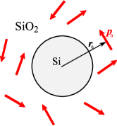
Figure 1: Schematic illustration of the Si QD surrounded by randomly oriented dipoles in SiO₂ matrix. The radius-vector $\bm{r}_{0}$ is shown for one of the dipoles $\bm{p}_{0}$.

II Interaction of confined electrons with local vibrations of a polar glass

Let us consider a spherical semiconductor nanocrystal embedded into a polar glass matrix. We will characterize the $j$th local vibration mode in the glass by the oscillating dipole moment

$${\bm{p}}^{(j)}_{0}(t)=\sum\limits_{i}e_{i}^{(j)}\,{\bm{u}}_{i}^{(j)}(t)\,,$$

where $e_{i}^{(j)}$ and ${\bm{u}}_{i}^{(j)}(t)$ are the charge and the displacement of the $i$-th ion participating in the $j$-th local vibration. The system under study is sketched in Fig. 1, where a random orientation of the dipoles is assumed.

According to electrostatic approximation (see Appendix) the potential inside the nanocrystal of the radius $R$ and dielectric constant $\varepsilon_{\rm in}$ induced by a point dipole source with polarization $\bm{p}^{(j)}_{0}\delta(\bm{r}-\bm{r}_{0}^{(j)})$, positioned in the matrix with dielectric constant $\varepsilon_{\rm out}$, can be represented as

$$\varphi\left(\bm{r},{\bm{r}}_{0}^{(j)},{\bm{p}}_{0}^{(j)}\right)=\sum\limits_{JM}\frac{\alpha_{J}r^{J}}{\left[r_{0}^{(j)}\right]^{J+2}}\left[\bm{p}_{0}^{(j)}\cdot\bm{Y}_{JM}^{J+1}\left({\bm{n}}_{0}^{(j)}\right)\right]^{*}\>,$$ (1)

where

$$\alpha_{J}=\frac{4\pi\sqrt{(J+1)(2J+1)}}{\varepsilon_{\rm in}J+\varepsilon_{\rm out}(J+1)},\>{\bm{n}}_{0}^{(j)}=\frac{{\bm{r}}_{0}^{(j)}}{r_{0}^{(j)}}\,,$$ (2)

and $\bm{Y}_{JM}^{L}(\bm{n})$ are the vector spherical harmonics introduced in Ref. vmk, .

Neglecting retardation, one can use the Fermi golden rule to calculate the rate of intraband transitions of the electron confined within the spherical nanocrystal under the influence of the quasistatic electric field induced by the local vibrations. At low temperatures lowT this rate is given by

$$\begin{split}\frac{1}{\tau}=\frac{2\pi}{\hbar}\sum\limits_{j}|\langle\psi_{f}|e\varphi(\bm{r}_{0}^{(j)}&,{\bm{p}}_{0}^{(j)})|\psi_{i}\rangle|^{2}\times\\ \,&\delta(E_{i}-E_{f}-\hbar\omega_{\rm ph}^{(j)})\,,\end{split}$$ (3)

where summation runs over all the local modes of the matrix, $E_{i}$ and $E_{f}$ are, respectively, the energies of the initial $|\psi_{i}\rangle$ and the final $|\psi_{f}\rangle$ states of the confined electron. Neglecting electron tunneling outside the sphere, one can write the transition matrix element as

$$\begin{split}&\langle\psi_{f}|e\varphi({\bm{r}}_{0}^{(j)},{\bm{p}}_{0}^{(j)})|\psi_{i}\rangle=\\ &e\sum\limits_{JM}\frac{\alpha_{J}}{\left[r_{0}^{(j)}\right]^{J+2}}\langle\psi_{f}|r^{J}Y_{JM}|\psi\rangle\left[\bm{p}_{0}^{(j)}\cdot\bm{Y}_{JM}^{J+1}\left({\bm{n}}_{0}^{(j)}\right)\right]^{*}\>.\end{split}$$ (4)

Introducing the vibration distribution function as

$$P({\bm{r}}_{0},{\bm{p}},\omega)\equiv P_{0}\,\frac{1}{4\pi}\frac{\delta(p-p_{0})}{p_{0}^{2}}\,\rho(\omega)$$

(where $P_{0}=\rm const$) summation over vibrational modes in Eq. (3) can be reduced to

$$\begin{split}\frac{1}{\tau}=\frac{2\pi}{\hbar}&\rho\left(\tfrac{E_{i}-E_{f}}{\hbar}\right)P_{0}\times\\ &\int d{\bm{r}}_{0}\int\frac{d\Omega_{{\bm{p}}_{0}}}{4\pi}|\langle\psi_{f}|e\varphi(\bm{r}_{0},{\bm{p}}_{0})|\psi_{i}\rangle|^{2}\,.\end{split}$$ (5)

The angular integration can be done with the help of

$$\iint d\Omega_{{\bm{p}}_{0}}d\Omega_{{\bm{r}}_{0}}[\bm{p}_{0}\cdot\bm{Y}_{JM}^{J+1}(\Omega_{{\bm{r}}_{0}})]\cdot[\bm{p}_{0}\cdot\bm{Y}_{J^{\prime}M^{\prime}}^{J^{\prime}+1}(\Omega_{{\bm{r}}_{0}})]^{*} =$$

$$\frac{4\pi}{3}p_{0}^{2}\delta_{JJ^{\prime}}\delta_{MM^{\prime}}.$$ (6)

Thus, finally we get

$$\frac{1}{\tau}=\frac{2\pi}{\hbar}\rho\left(\tfrac{E_{i}-E_{f}}{\hbar}\right)P_{0}\,|\langle\psi_{f}|e\varphi(r_{0})|\psi_{i}\rangle|^{2}\,,$$ (7)

where

$$|\langle\psi_{f}|e\varphi(r_{0})|\psi_{i}\rangle|^{2}\equiv\\ \frac{1}{4\pi}\int d\Omega_{{\bm{p}}_{0}}\int d\Omega_{{\bm{r}}_{0}}|\langle\psi_{f}|e\varphi(\bm{r}_{0},{\bm{p}}_{0})|\psi_{i}\rangle|^{2}=\\ \frac{e^{2}p_{0}^{2}}{3}\sum\limits_{JM}\frac{\alpha_{J}^{2}}{2J+1}\frac{1}{r_{0}^{2J+4}}|\langle\psi_{f}|r^{J}Y_{JM}|\psi_{i}\rangle|^{2}\>.$$ (8)

III Discussion

We need to estimate the mean value of the dipole moment corresponding to a given local vibrational mode. Let us first introduce characteristic values, $u$ and $M_{0}$, for the mean square displacement and atomic mass of the atoms participating in the vibration, respectively (we neglect the fact that we deal with different sorts of atoms). This enables us to write

$$\sum\limits_{i=1}^{N}M_{i}\langle u_{i}^{(j)\,2}\rangle\omega_{\rm ph}^{(j)\,2}\sim NM_{0}u^{2}\omega_{\rm ph}^{2}\,,$$

where $N$ is the number of atoms participating in the vibration, $\omega_{\rm ph}\equiv\omega_{\rm ph}^{(j)}$. At low temperatures

$$NM_{0}u^{2}\omega_{\rm ph}^{2}\sim\hbar\omega_{\rm ph}\,,$$

and, therefore,

$$u\sim\sqrt{\frac{\hbar}{NM_{0}\omega_{\rm ph}}}\>.$$ (9)

The dipole moment characterizing this vibrational mode is related to $u$ through

$$p\sim eu\gamma\,,$$ (10)

where the factor $\gamma$ depends on the relative orientations of displacements for atoms participating in the local mode.gamma,

The other glass parameters entering Eq. (7) are the concentration of dipoles, $P_{0}$, and vibrational density of states, $\rho$ . The concentration of dipoles is of the order of

$$P_{0}\sim a^{-3}N^{-1},$$ (11)

where $a$ is the characteristic atomic scale. The rough estimation for the density of states is $\rho\sim 1/(\hbar\omega_{\rm ph})$. Numerical simulations performed for silica glass  taraskin1, ; taraskin2, ; olig, show that the actual phase volume of the high-frequency localized vibrations is at least by a factor of 5 less than the total phase volume. This factor decreases the density of states by about an order of magnitude.

IV Model calculation

In this Section we will perform a model calculation of the relaxation time due to the coupling of electron confined in a quantum dot with local vibrations of the quantum dot environment. The quantum dot is treated as a spherical quantum well with the infinite potential barrier. We consider an electron from a simple band with an isotropic effective mass $m^{*}$ and use the effective mass approximation. In this case the electron states are characterized by the radial quantum number $n$, the orbital angular momentum $l$, its projection $m$ onto an arbitrary axis, and a projection of the electron spin. Neglecting for simplicity the electron spin, within the effective mass approximation one can characterize the electron states only by the envelope wave function

$$\psi_{nlm}(\bm{r})=\sqrt{\frac{2}{R^{3}}}Y_{lm}(\theta,\varphi)\frac{j_{l}(\varphi_{nl}r/R)}{j_{l+1}(\varphi_{nl})}$$ (12)

where $j_{l}(x)$ is the spherical Bessel function, the numbers $\varphi_{nl}$ are found from

$$j_{l}(\varphi_{nl})=0,$$

and the energy levels

$$\quad E_{nl}=\frac{\hbar^{2}}{2m^{*}R^{2}}\varphi_{nl}^{2}$$ (13)

are degenerate over $m$. zeros, Fig. 2 shows the dependence of first six energy levels on the nanocrystal diameter, $2R$, for $2R>4$ nm, where the density of states mass in Si, $m^{*}=0.33\,m_{0}$ was used ($m_{0}$ is the free electron mass). Comparison of the energy level positions with those provided by more accurate calculations andrei1, ; andrei2, suggests that the approximation of infinite barriers is reasonable for the dot under consideration.

A transition between two of the levels of size quantization with the energies (13) is possible when their diameter-dependent difference falls within the spectral range,

$$120~{}{\rm meV}\lesssim\hbar\omega_{\rm ph}\lesssim 160~{}{\rm meV}\>,$$ (14)

corresponding to high-frequency local vibrations of the silica glass taraskin1, ; taraskin2, ; olig, . Vertical arrows in Fig. 2 indicate these allowed regions and the corresponding transition time is shown near each arrow. The calculation is carried out for the set of QD parameters close to that of Si/SiO₂ system: $\varepsilon_{\rm in}=3$, $\varepsilon_{\rm out}=12$. Our model is too simple to describe the spectral dependence of glass parameters. Thus, we take them at a fixed value in the middle of the range (14): $\hbar\omega_{\rm ph}=140$ meV. Other parameters used are as follows: $N=15$, $\gamma=\sqrt{N}$, $P_{0}=(1/N)\cdot 1.5\times 10^{22}$ cm^-3 and $\rho(\hbar\omega)=1/(5\hbar\omega_{\rm ph})$. The vibrating mass, $M_{0}$, was taken as $M_{0}=(1/3)M_{\rm Si}+(2/3)M_{\rm O}$ where $M_{\rm Si}$ and $M_{\rm O}$ are the silicon and oxygen atomic masses, respectively. Since the levels (13) are degenerate over momentum projection $m$, we have summed the relaxation rate (7) over the final states and averaged over initial ones.

Fig. 2 demonstrates that typical value of the relaxation time is of the order of 1 ns. The transition rate is proportional to $1/R$, so it changes with the nanocrystal diameter slower than the energy difference proportional to $1/R^{2}$.

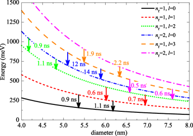
Figure 2: Relaxation time between the first six energy levels for different diameters of the nanocrystal. The values of $n_{r}$ and $l$ are shown for each curve. The transition time for the corresponding levels at given diameter is indicated near the vertical arrows.

V Conclusions

We have shown that interaction of electrons confined in a non-polar quantum dot with local vibrations of amorphous polar environment provides an efficient energy relaxation channel for the “hot” electrons. We demonstrated that this mechanism controls energy relaxation in Si nanocrystals in SiO₂ matrix with diameters in the range of $4$ – $8$ nm, where the energy relaxation process can proceed through emission of a single phonon. In this case the relaxation time is in nanosecond range. Energy relaxation in quantum dots with smaller diameters should be controlled by multiphonon processes. We expect nonradiative relaxation there to be slower with the rate comparable to that of radiative intraband transitions.emrs ; delerue

This work was supported in part by the Russian Foundation for Basic Research and by DoD under contract No. W912HZ-06-C-0057. A.N.P. also acknowledges the support of the “Dynasty” Foundation-ICFPM.

Appendix

Let us calculate electric filed induced by a point dipole $\bm{p}_{0}$ positioned at at the point $\bm{r}_{0}$ outside the sphere of radius $R$. Dielectric constants inside and outside the sphere are $\varepsilon_{\rm in}$ and $\varepsilon_{\rm out}$, respectively. We are interested in the field inside the sphere. Within electrostatic approximation the electric field $\bm{E}$ can be expressed via the scalar potential $\varphi$ as

$$\bm{E}=-\mathop{\mathrm{missing}}{grad}\nolimits\varphi.$$ (A1)

The Poisson equation for the potential $\varphi$ reads

$$\Delta\varphi=\frac{4\pi}{\varepsilon_{\rm out}}\mathop{\mathrm{missing}}{div}\nolimits[\bm{p}_{0}\delta(\bm{r}-\bm{r}_{0})],\quad(r_{0}>R),$$ (A2)

and the boundary conditions at the sphere surface are

$$\varphi|_{r=R-0}=\varphi|_{r=R+0},$$ (A3)

$$\varepsilon_{\rm in}\frac{\partial\varphi}{\partial r}\Bigl{|}_{r=R-0}=\varepsilon_{\rm out}\frac{\partial\varphi}{\partial r}\Bigl{|}_{r=R+0}\>.$$

In the case of homogeneous medium ($\varepsilon_{\rm in}=\varepsilon_{\rm out}$) the solution of (A2) is obvious,

$$\varphi_{0}(\bm{r})=-\frac{1}{\varepsilon_{\rm out}}\mathop{\mathrm{missing}}{div}\nolimits\frac{\bm{p}_{0}}{|\bm{r}-\bm{r}_{0}|}\>.$$ (A4)

In what follows it is convenient to use the basis of vector spherical harmonics $\bm{Y}_{JM}^{L}(\theta,\varphi)$ vmk,  . The identity

$$\begin{split}\frac{\bm{p}_{0}}{|\bm{r}-\bm{r}_{0}|}=\sum\limits_{JLM}\frac{4\pi}{2L+1}\frac{r_{<}^{L}}{r_{>}^{L+1}}\bm{Y}_{JM}^{L}(\bm{n})[\bm{Y}_{JM}^{L*}(\bm{n}_{0})\cdot\bm{p}_{0}],\end{split}$$

where $r_{>}=\max(r,r_{0}),r_{<}=\min(r,r_{0}),\bm{n}=\bm{r}/r,\bm{n}_{0}=\bm{r}_{0}/r_{0}$ is useful to present (A4) as a sum of scalar spherical harmonics $Y_{JM}$. After calculating the derivatives we obtain

$$\varphi_{0}(\bm{r})=\begin{cases}\sum\limits_{JM}\displaystyle\frac{r^{J}}{r_{0}^{J+2}}Y_{JM}(\bm{n})\xi_{JM},\quad r<r_{0}\\ \sum\limits_{JM}\displaystyle\frac{r_{0}^{J-1}}{r^{J+1}}Y_{JM}(\bm{n})\eta_{JM},\quad r>r_{0}\end{cases}$$ (A5)

with

$$\xi_{JM}=\frac{4\pi}{\varepsilon_{\rm out}}\sqrt{\frac{J+1}{2J+1}}[\bm{p}_{0}\cdot\bm{Y}_{JM}^{J+1}(\bm{n}_{0})]^{*},$$ (A6)

$$\quad\eta_{JM}=\frac{4\pi}{\varepsilon_{\rm out}}\sqrt{\frac{J}{2J+1}}[\bm{p}_{0}\cdot\bm{Y}_{JM}^{J-1}(\bm{n}_{0})]^{*}\>.$$ (A7)

When $\varepsilon_{\rm in}\neq\varepsilon_{\rm out}$ the scalar potential can be written as

$$\varphi(r)=\begin{cases}\sum\limits_{JM}r_{JM}Y_{JM}(\bm{n})\displaystyle\frac{R^{J}}{r^{J+1}}+\varphi_{0}(\bm{r}),&(r>R)\\ \sum\limits_{JM}t_{JM}Y_{JM}(\bm{n})\displaystyle\frac{r^{J}}{R^{J+1}},&(r<R)\>.\end{cases}$$ (A8)

Substituting (A8) and (A6) into the boundary conditions (A3) we find the coefficients $t_{JM}$ and $t_{JM}$:

$$t_{JM}=\xi_{JM}\frac{R^{J+1}}{r_{0}^{J+2}}\frac{(2J+1)\varepsilon_{\rm out}}{\varepsilon_{\rm in}J+\varepsilon_{\rm out}(J+1)},$$ (A9)

$$r_{JM}=\xi_{JM}\frac{R^{J+1}}{r_{0}^{J+2}}\frac{J(\varepsilon_{\rm out}-\varepsilon_{\rm in})}{\varepsilon_{\rm in}J+\varepsilon_{\rm out}(J+1)}\>,$$ (A10)

which allows to express the scalar potential as (1) .

References

- (1) B.K. Ridley, Phys. Rev. B 47, 4592 (1993).
- (2) R. Lassnig, Phys. Rev. B 30, 7132 (1984).
- (3) M.C. Klein, F. Hache, D. Ricard, and C. Flytzanis, Phys. Rev. B 42, 11123 (1990).
- (4) E. Roca, C. Trallero-Giner, and M. Cardona, Phys. Rev. B 49, 13704 (1994).
- (5) A. J. Kenyon, Prog. Quantum Electron. 26, 225 (2002).
- (6) L. Pavesi, L. Dal Negro, C. Mazzoleni, G. Franzo, F. Priolo, Nature 408, 440 (2000).
- (7) D. Timmerman, I. Izeddin, P. Stallinga, I. N. Yassievich, T. Gregorkiewicz, Nature Photonics 2, 105 (2008).
- (8) S.N. Taraskin and S.R. Elliott, Phys. Rev. B 56, 8605 (1997).
- (9) S.N. Taraskin and S.R. Elliott, Phys. Rev. B 59, 8572 (1999).
- (10) C. Oligschleger, Phys. Rev. B 60, 3182 (1999).
- (11) G.L. Bir and G.E. Pikus, Symmetry and Strain-Induced Effects in Semiconductors (Wiley, New York 1974).
- (12) D.A. Varshalovich, A.N. Moskalev, and V.K. Khersonskii, Quantum Theory of Angular Momentum (World Scientific, Singapore, 1988).
- (13) As the characteristical energies of local vibrations meVolig , the high-temperature range is out of interest .
- (14) In the limiting case when the dipole characterizing a given vibrational mode can be represented as elementary dipoles oscillating in phase, . We expect that randomization of phases would lead to .
- (15) S. Flügge, Practical quantum mechanics I (Springer-Verlag, Berlin – Heidelberg – New-York, 1971).
- (16) A.S. Moskalenko and I.N. Yassievich, Phys. Solid State 46, 1508 (2004).
- (17) A.S. Moskalenko, I.N. Yassievich, M. Forcales, M. Klik, and T. Gregorkiewicz, Phys. Rev. B 70, 155201 (2004).
- (18) A.A. Prokofiev, S.V. Goupalov, A.S. Moskalenko, A.N. Poddubny, I.N. Yassievich, arXiv:0805.3451v1, to be published in Physica E (2008).
- (19) G. Allan and C. Delerue, Phys. Rev. B 66, 233303 (2002) .