Structural approximations to positive maps and entanglement breaking channels

Abstract

Structural approximations to positive, but not completely positive maps are approximate physical realizations of these non-physical maps. They find applications in the design of direct entanglement detection methods. We show that many of these approximations, in the relevant case of optimal positive maps, define an entanglement breaking channel and, consequently, can be implemented via a measurement and state-preparation protocol. We also show how our findings can be useful for the design of better and simpler direct entanglement detection methods.

I Introduction

Entanglement is one of the most important, and presumably necessary, ingredients of quantum information processing review-horo . For this reason there is a considerable interest both in theory and experiments in designing feasible and efficient ways of entanglement detection. Indeed, there has been a lot of progress in this problem recently. The most frequently used and investigated entanglement detection methods include: i) tomography of the quantum state with local measurements, useful for low dimensional systems provided entanglement criteria for the states in question are known white98 ; blatt1 ; blatt2 , but impractical for higher dimensional systems; ii) methods based on detecting only some elements of the density matrix for a continuous family of measuring devices settings, such as the method of entanglement visibility visibility ; iv) tests of generalized Bell inequalities Bell , although there are states that despite being entangled do not violate any Bell inequality Werner ; lhv nor any known Bell inequality reviewbell ; v) entanglement witnesses horo96 ; terhal ; vi) direct entanglement detection schemes, for pure huelga or mixed states Mintert and, in particular, using structural approximations to positive maps pawel ; pawel_ekert ; vii) “nonlinear” entanglement witnesses guehne1 and viii) methods employing measurements of variances guehne2 or even higher order correlation functions korbicz ; blatt2 , or relying on entropic uncertainty relations guehne3 . The methods v) and vi) are the subject of the present paper and we discuss them in more detail below. First we recall some basic definitions.

Entanglement Witnesses.

An observable $E=E^{{\dagger}}$ is called an entanglement witness if and only if, for all separable states $\sigma$, the average $\text{tr}(E\sigma)\geq 0$ and there exists an entangled state $\varrho$ for which $\text{tr}(E\varrho)<0$. As shown in Ref. horo96 , the Hahn-Banach theorem implies that for every entangled state $\varrho$, there exists a witness $E$ that detects it, i.e. $\text{tr}(E\varrho)<0$. Conversely, the state $\sigma$ is separable if and only if for all witnesses it holds $\text{tr}(E\sigma)\geq 0$. As has been pointed out in Ref. guehnepra , entanglement witnesses can be efficiently measured with local measurements and, more importantly, one can optimize the complexity of this measurement with respect to, for instance, the number of measuring device settings. Nowadays, entanglement witnesses are routinely used in experiments to detect entanglement in bipartite demartini and multipartite blatt1 ; harald systems.

Positive Maps.

A related concept is that of a positive map. Let $\mathcal{B}(\mathcal{H}_{A})$ and $\mathcal{B}(\mathcal{H}_{B})$ denote the spaces of bounded operators on Hilbert spaces $\mathcal{H}_{A}$ and $\mathcal{H}_{B}$ respectively. Then a linear map $\Lambda\colon\mathcal{B}(\mathcal{H}_{A})\to\mathcal{B}(\mathcal{H}_{B})$ is called positive if $\Lambda(\varrho)\geq 0$ for every $\varrho\geq 0$. However, not every positive map can be regarded as physical, describing e.g. a quantum channel or the reduced dynamics of an open system: a stronger positivity condition is required Kraus . Namely, a map $\Lambda$ is physical whenever it is completely positive, which means that the extended map ${\bf 1}\otimes\Lambda\colon\mathcal{B}(\mathcal{K}\otimes\mathcal{H}_{A})\to\mathcal{B}(\mathcal{K}\otimes\mathcal{H}_{B})$ is positive for any extension $\mathcal{K}$.

Again, as shown in Ref. horo96 (see also Woronowicz ), a state $\varrho\in\mathcal{B}(\mathcal{H}_{A}\otimes\mathcal{H}_{B})$ is entangled if and only if there exists a positive, not completely positive map $\Lambda\colon\mathcal{B}(\mathcal{H}_{B})\to\mathcal{B}(\mathcal{H}_{A})$ that detects $\varrho$, i.e. $[{\bf 1}\otimes\Lambda](\varrho)$ is not positive definite. A paradigm example of a positive but not completely positive map is transposition, $T$, whose great significance for separability was first realized in Ref. PPT . It turns out to detect all the entangled states in $\mathcal{B}(\mathbb{C}^{2}\otimes\mathbb{C}^{2})$ and $\mathcal{B}(\mathbb{C}^{2}\otimes\mathbb{C}^{3})$ horo96 . However, as it is well known be (see also e.g. Ref. review-horo and references therein), in higher dimensions there are entangled states which possess the positive partial transpose (PPT) property.

Entanglement witnesses and positive maps notepos are related through the Jamiołkowski isomorphism jam . Let $E\in\mathcal{B}(\mathcal{H}_{A}\otimes\mathcal{H}_{B})$. From this moment on we assume that the considered Hilbert spaces are finite dimensional, $\text{dim}\mathcal{H}_{A,B}=d_{A,B}<\infty$ (for an example of infinite dimensional generalization of Jamiołkowski isomorphism see Ref. cmp ). We then define $\Lambda_{E}\colon\mathcal{B}(\mathcal{H}_{A})\to\mathcal{B}(\mathcal{H}_{B})$ as follows:

$$\Lambda_{E}(\varrho)=d_{A}\text{tr}_{A}\left[E(\varrho^{T}\otimes{\bf 1})\right].$$ (1)

Conversely, introducing a maximally entangled vector in $\mathcal{H}_{A}\otimes\mathcal{H}_{A}$,

$$|\Phi_{+}\rangle=\frac{1}{\sqrt{d_{A}}}\sum_{i=1}^{d_{A}}|ii\rangle,\quad P_{+}=|\Phi_{+}\rangle\langle\Phi_{+}|$$ (2)

we define for each map $\Lambda\colon\mathcal{B}(\mathcal{H}_{A})\to\mathcal{B}(\mathcal{H}_{B})$ an operator

$$E_{\Lambda}={\bf 1}\otimes\Lambda(P_{+})$$ (3)

acting on $\mathcal{B}(\mathcal{H}_{A}\otimes\mathcal{H}_{B})$. Then $\Lambda$ is positive if and only if $E_{\Lambda}$ is an entanglement witness, since $E_{\Lambda_{E}}=E$ jam . Moreover, $\Lambda$ is completely positive if and only if $E_{\Lambda}\geq 0$, i.e. $E_{\Lambda}$ is a (possibly unnormalized) state.

Structural Physical Approximation.

Positive maps are stronger detectors of entanglement than the corresponding witnesses, despite the described Jamiołkowski isomorphism. They detect the same states as the corresponding witnesses plus those obtained through local invertible transformation on one side. Unfortunately generic positive maps are not physical and their action cannot be directly implemented. It is therefore challenging to try to find a physical way to approximate the action of a positive map. This is the goal of the structural physical approximation pawel ; pawel_ekert . The idea is to mix a positive map $\Lambda$ with some simple completely positive map (CPM), making the mixture $\tilde{\Lambda}$ completely positive. The resulting map can then be realized in the laboratory and its action characterizes entanglement of the states detected by $\Lambda$. In the particular example studied in Refs. pawel ; pawel_ekert this idea has been applied to the map $\Lambda={\bf 1}\otimes T$. Although experimentally viable, this method is not easy to implement since, at least in its original version, it requires highly nonlocal measurements: subsequent applications of $\tilde{\Lambda}$ followed by optimal spectrum estimation. A more detailed discussion on this entanglement detection scheme is given in Section V.

In the case of finite dimensional Hilbert spaces, we can, without lost of generality, restrict our attention to contractive structural approximations, i.e. ${\rm tr}(\tilde{\Lambda}(\varrho))\leq 1$, for $\text{tr}(\varrho)=1$. If the initial map is not contractive, we can always define $\tilde{\Lambda}^{\prime}(\varrho)=\tilde{\Lambda}(\varrho)/{\rm tr}(\tilde{\Lambda}(\varrho^{*}))$, where ${\rm tr}(\tilde{\Lambda}(\varrho^{*}))=\max_{\varrho:\text{tr}(\varrho)=1}{\rm tr}(\tilde{\Lambda}(\varrho))$) and the maximum is attained for some $\varrho^{*}$ due to the compactness of the set of all states. Contractive CPM’s can be realized probabilistically as a partial result of a generalized measurement (see Ref. pawel ).

Entanglement Breaking Channels.

A different use of maps in the context of quantum theory concerns the description of quantum channels, which are completely positive and trace-preserving maps. A channel $\Lambda$ that transforms any state $\varrho$ into a separable state $\Lambda(\varrho)$ is called entanglement breaking (EB) ruskai . Clearly, these channels are useless for entanglement distribution. In Ref. ruskai , the following equivalence was obtained:

1. The channel $\Lambda$ is EB.

2. The corresponding state $E_{\Lambda}$ is separable.

3. The channel can be represented in the Holevo form:

   $$\Lambda(\varrho)=\sum_{k}\text{tr}(F_{k}\varrho)\varrho_{k},$$ (4)

   with some positive operators $F_{k}\geq 0$ defining a generalized measurement peresbook , $\sum_{k}F_{k}={\bf 1}$, and states $\varrho_{k}$ determined only by $\Lambda$.

The last property above means that the action of an EB channel can be substituted by a measurement and state-preparation protocol. Moreover, from the separable decomposition of the state $E_{\Lambda}$

$$E_{\Lambda}=\sum_{k}p_{k}|v_{k}\rangle\langle v_{k}|\otimes|w_{k}\rangle\langle w_{k}|$$ (5)

with $|v_{k}\rangle\in\mathcal{H}_{A}$ and $|w_{k}\rangle\in\mathcal{H}_{B}$, one obtains the following explicit Holevo representation of $\Lambda$ ruskai :

$$\Lambda(\varrho)=\sum_{k}|w_{k}\rangle\langle w_{k}|\text{tr}\Big{[}\left(d_{A}p_{k}|\bar{v_{k}}\rangle\langle\bar{v_{k}}|\right)\varrho\Big{]},$$ (6)

where the overbar denotes the complex conjugation. The positive operators $\{d_{A}p_{k}|\bar{v}_{k}\rangle\langle\bar{v}_{k}|\}$ define a properly normalized measurement due to the trace-preserving property of $\Lambda$.

Notice that these results can easily be extended to the case of contracting maps. Then, a Holevo decomposition is still possible for EB maps with the positive operators $F_{k}$ defining a partial measurement, $\sum_{k}F_{k}<{\bf 1}$.

In this paper we address the question of implementation of structural approximations to positive maps through (generalized) measurements. In particular, we study structural approximations to maps $\Lambda\colon\mathcal{B}(\mathcal{H}_{A})\to\mathcal{B}(\mathcal{H}_{B})$ obtained through minimal admixing of white noise:

$$\widetilde{\Lambda}(\rho)=p\,\text{tr}(\rho)\frac{\bf 1}{d_{B}}+(1-p)\Lambda(\rho).$$ (7)

Minimal means here that we take the smallest noise probability $0<p<1$ for which $\tilde{\Lambda}$ becomes completely positive. Now the key question is when such $\tilde{\Lambda}$ can be implemented through generalized measurements, i.e. when they correspond to EB maps according to Eq. (4). As a consequence, we are led to study the separability of witnesses of the form

$$\widetilde{E}_{\Lambda}={\bf 1}\otimes\widetilde{\Lambda}(P_{+})=\frac{p}{d_{A}d_{B}}{\bf 1}+(1-p)E_{\Lambda}$$ (8)

for minimal $p$ such that

$$\widetilde{E}_{\Lambda}\geq 0.$$ (9)

Recall that this is equivalent to $\widetilde{\Lambda}$ being completely positive. In general, we will consider contractive maps $\tilde{\Lambda}$ and ask whether they correspond to EB maps, not necessarily trace-preserving. Note that if a CPM $\tilde{\Lambda}$ is contractive and EB, then there exists an EB extension to a trace-preserving map, $\tilde{\Lambda}^{\prime}(\varrho)=\tilde{\Lambda}(\varrho)+[{\rm tr}(\varrho)-{\rm tr}(\tilde{\Lambda}(\varrho))]{\bf 1}/d$. In the language of witnesses, trace preservation means ${\rm tr}_{B}E_{\tilde{\Lambda}}={\bf 1}_{A}$.

The main subject of the paper is the following conjecture:

Conjecture: Structural physical approximations to optimal positive maps correspond to entanglement breaking maps. Equivalently, structural physical approximations to optimal entanglement witnesses $E$ are given by (possibly unnormalized) separable states.

We prove the above conjecture in several special cases and discuss a large number of generic examples providing evidence for its validity. This is done for both decomposable entanglement witnesses, that detect only entangled states with negative partial transposition (NPT), and also for non-decomposable witnesses which in addition detect PPT entangled states. Once more, we expect the conjecture to be valid in general, but in some cases we restrict our examples to structural approximations which are trace-preserving. Note that such restriction makes the conjecture weaker, since every contractive EB channel has a trace preserving EB extension, but not vice-versa.

The importance of our result is twofold: i) if the conjecture is true, structural physical approximations to optimal maps admit a particularly simple experimental realization—they correspond to generalized measurements remik ; ii) the results shed light on the geometry of the set of entangled and separable states (cf. Ref. karol ).

The paper is organized as follows. In Section II we recall the notions of decomposable and non-decomposable entanglement witnesses and their optimality, based on the Refs. opt1 ; opt2 . In Section III we concentrate on decomposable maps. First we study dimensions $2\otimes 2$ and $2\otimes 3$, where the positivity of the partial transpose provides the separability criterion. Here we show that in general, without the assumption of optimality, the conjecture is not true, while it obviously holds for optimal decomposable witnesses. Next, we discuss general decomposable maps in $2\otimes 4$ systems, which are nontrivial due to the existence of PPT entangled states. Other examples of maps in $3\otimes 3$ systems satisfying the conjecture are presented in Appendix B. We conclude this section proving the conjecture for the transposition and reduction map reduction in arbitrary dimension. Section IV is devoted to non-decomposable positive maps. We start the discussion by analyzing the case of Choi’s map, one of the first examples of a map in this class. Then, we study a positive map based on unextendible product bases (UPB’s) terhal_upb . Finally, we end this section with an analysis of the Breuer-Hall map Breuer ; Hall , which can be understood as the non-decomposable version of the reduction criterion. Here symmetry methods turn out to be indispensable. We introduce and study in some detail a new family of states—unitary symplectic invariant states. The most technical details of these states are mainly given in Appendix C, where, as a byproduct, we show that this family includes also bound entangled states. Finally, we study the physical approximation to partial transposition, as this map is used in the direct entanglement detection method proposed in pawel_ekert . In the latter case the analysis is again made possible due to symmetry arguments, in particular the unitary $U\bar{U}VV$ symmetry (cf. Refs. werner_sym ; masanes ). The paper ends with the conclusions in Section VI.

II Optimality of Positive Maps and Entanglement Witnesses

The notion of optimality of positive maps and entanglement witnesses has been introduced in Refs. opt1 ; opt2 . We review it here without proofs, which can be found in the original papers. There are two concepts of optimality: one general, and one strictly related to non-decomposable positive maps (or entanglement witnesses) and PPT entangled states. We focus below on entanglement witnesses—the translation to positive maps is straightforward using the Jamiołkowski’s isomorphism (cf. Eqs. (1) and (3)).

II.1 General Optimality

Let us introduce the notion of general optimality first. Given an entanglement witness $E$ we define:

• $D_{E}=\{\varrho\geq 0:\text{tr}(E\varrho)<0\}$—the set of operators detected by $E$.

• Finer witness — given two witnesses $E_{1}$ and $E_{2}$ we say that $E_{2}$ is finer than $E_{1}$, if $D_{E_{1}}\subset D_{E_{2}}$, i.e. if all the operators detected by $E_{1}$ are also detected by $E_{2}$.

• Optimal witness — $E$ is optimal if there exists no other witness which is finer than $E$.

• $P_{E}=\{u\otimes v\in\mathcal{H}_{A}\otimes\mathcal{H}_{B}:\langle u\otimes v|Eu\otimes v\rangle=0\}$ — the set of product vectors on which $E$ vanishes. As we will show, these vectors are closely related to the optimality property.

Vectors in $P_{E}$ play an important role regarding entanglement. A full characterization of optimal witnesses is provided by the following theorem:

Theorem 1: A witness $E$ is optimal if and only if for all operators $P\geq 0$ and numbers $\epsilon>0$, $E^{\prime}=E-\epsilon P$ is not an entanglement witness.

In this paper we will use the following important corollary:

Corollary 2: If the set $P_{E}$ spans the whole Hilbert space $\mathcal{H}_{A}\otimes\mathcal{H}_{B}$, then $E$ is optimal.

II.2 Decomposable witnesses

There exists a class of entanglement witnesses which is very simple to characterize—decomposable entanglement witnesses Woronowicz . Those are the witnesses which can be written in the form:

$$E=Q_{1}+Q_{2}^{\Gamma},$$ (10)

where $Q_{1,2}\geq 0$ and $\Gamma$ refers to partial transposition with respect to the second subsystem:

$$Q^{\Gamma}=({\bf 1}\otimes T)Q.$$ (11)

As it is well known, these witnesses cannot detect PPT entangled states. We recall here some simple properties of optimal decomposable entanglement witnesses:

Theorem 2: Let $E$ be a decomposable witness. If $E$ is optimal then it can be written as $E=Q^{\Gamma}$, where $Q\geq 0$ contains no product vector in its range.

This result can be slightly generalized as follows:

Theorem 2’: Let $E$ be a decomposable witness. If $E$ is optimal then it can be written as $E=Q^{\Gamma}$, where $Q\geq 0$ and there is no operator $P$ in the range of $Q$ such that $P^{\Gamma}\geq 0$.

II.3 Non-decomposable witnesses

Entanglement witnesses which are able to detect PPT entangled states cannot be written in the form (10) Woronowicz , and are therefore called non-decomposable. The present Subsection is devoted to this kind of witnesses. The importance of non-decomposable witnesses for detecting PPT entanglement is reflected by the following:

Theorem 3: An entanglement witness is non–decomposable if and only if it detects some PPT entangled state.

We now recall some definitions which are parallel to those provided previously. Given a non-decomposable witness $E$, we define:

• $d_{E}=\{\varrho\geq 0:\varrho^{\Gamma}\geq 0{\mbox{ and }}\text{tr}(E\varrho)<0\}$ — the set of PPT operators detected by $E$.

• Finer non-decomposable witness—given two non-decomposable witnesses $E_{1}$ and $E_{2}$ we say that $E_{2}$ is nd–finer than $E_{1}$ if $d_{E_{1}}\subset d_{E_{2}}$, i.e. if all PPT operators detected by $E_{1}$ are also detected by $E_{2}$.

• Optimal non-decomposable witness — $E$ is optimal non-decomposable if there exists no other non-decomposable witness which is nd-finer than $E$.

Again, vectors in $P_{E}$ play an important role regarding PPT entangled states. The full characterization of optimal non-decomposable witnesses is given by an analog of Theorem 1:

Theorem 4: A non-decomposable entanglement witness $E$ is optimal if and only if for all decomposable operators $D$ and $\epsilon>0$, $E^{\prime}=E-\epsilon D$ is not an entanglement witness.

Note that in principle non-decomposable optimality requires the witness to be finer with regard to PPT entangled states only, so that a non-decomposable optimal witness does not have to be optimal in the sense of Section II.1. However, this is not the case since we have the following:

Theorem 5: $E$ is an optimal non-decomposable entanglement witness if and only if both $E$ and $E^{\Gamma}$ are optimal witnesses.

and

Corollary 6: $E$ is an optimal non-decomposable witness if and only if $E^{\Gamma}$ is an optimal non-decomposable witness.

In Ref. opt1 optimality conditions have been derived and investigated for the case of $2\otimes N$-dimensional Hilbert spaces. These conditions are, however, very complex and for the purpose of the present work we will use Corollary 2 to check optimality, even though it provides only a sufficient condition.

III Decomposable maps

This section is devoted to the study of the conjecture for decomposable maps. We start by proving the conjecture for low dimensional systems, namely $2\otimes 2$ and $2\otimes 3$. Then, we provide some rather general results for $2\otimes 4$ systems. Moreover, Appendix B contains several relevant examples of decomposable maps in $3\otimes 3$ systems where the conjecture also holds. Finally, we prove the conjecture in arbitrary dimension for two of the most important examples of decomposable maps, the transposition and reduction maps.

III.1 $2\otimes 2$ and $2\otimes 3$

We begin with general examples in the lowest non-trivial dimensions. Take $\Lambda$ to be a positive map from $\mathcal{B}(\mathbb{C}^{2})$ to $\mathcal{B}(\mathbb{C}^{2})$ or to $\mathcal{B}(\mathbb{C}^{3})$. Recall Woronowicz that every such map is decomposable, i.e. is of the form $\Lambda=\Lambda^{CP}_{1}+T\circ\Lambda^{CP}_{2}$ and that its corresponding entanglement witness can be written as (10). We will first show that not every structural approximation to $\Lambda$ is entanglement breaking. In other words, the optimality of the positive map is essential for the conjecture. For definiteness’ sake we analyze the $2\otimes 2$-dimensional case, but the argument also holds in $2\otimes 3$ systems.

Let us consider the entanglement witness $E_{\Lambda}$ corresponding to $\Lambda$ and, $Q_{1}$ and $Q_{2}$ in (10) to be rank-one operators of the form:

$$Q_{2}=\left[\begin{array}[]{cccc}a&0&0&a\\ 0&0&0&0\\ 0&0&0&0\\ a&0&0&a\end{array}\right],\quad Q_{1}=\left[\begin{array}[]{cccc}0&0&0&0\\ 0&b&b&0\\ 0&b&b&0\\ 0&0&0&0\end{array}\right]$$ (12)

with real positive $a$ and $b$. Then the witness

$$Q_{1}+Q_{2}^{\Gamma}=\left[\begin{array}[]{cccc}a&0&0&0\\ 0&b&b+a&0\\ 0&b+a&b&0\\ 0&0&0&a\end{array}\right]$$ (13)

is not positive and therefore $\Lambda$ is not completely positive. From the general form (8) we obtain that:

$$\widetilde{E}_{\Lambda}= \frac{p}{4}{\bf 1}+(1-p)\big{(}Q_{1}+Q_{2}^{\Gamma}\big{)}$$ (18)

$$=\left[\begin{array}[]{cccc}a^{\prime}+c&0&0&0\\ 0&b^{\prime}+c&b^{\prime}+a^{\prime}&0\\ 0&b^{\prime}+a^{\prime}&b^{\prime}+c&0\\ 0&0&0&a^{\prime}+c\end{array}\right],$$

$$a^{\prime}= (1-p)a,\quad b^{\prime}=(1-p)b,\quad c=\frac{p}{4}.$$ (19)

This operator is positive for

$$p\geq\frac{4a}{4a+1},$$ (20)

which is the condition for the structural approximation.

In order to study separability, it is enough to check the PPT condition, as it is both a necessary and sufficient condition in the lowest dimensions PPT . Applying partial transposition we obtain that the state (18) is not PPT, and hence entangled, for

$$p<\frac{4b}{4b+1}.$$ (21)

Taking $b>a$ the condition (20) and (21) can be simultaneously satisfied, thus giving a structural approximation which is not entanglement breaking.

Above we have considered a general positive map from $\mathcal{B}(\mathbb{C}^{2})$ to $\mathcal{B}(\mathbb{C}^{2})$ or to $\mathcal{B}(\mathbb{C}^{3})$, i.e. $\Lambda=\Lambda^{CP}_{1}+T\circ\Lambda^{CP}_{2}$. Let us now consider an optimal one:

$$\Lambda=T\circ\Lambda^{CP},\quad E_{\Lambda}=Q^{\Gamma}.$$ (22)

It immediately follows that any structural approximation to such $\Lambda$ is entanglement breaking since

$$E_{\Lambda}^{\Gamma}=\frac{p}{4}{\bf 1}+(1-p)Q\geq 0,$$ (23)

so that $E_{\Lambda}$ is separable. Thus, in the lowest dimensions any structural approximation to an optimal map is entanglement breaking.

More generally, for arbitrary dimension we immediately obtain from Eq. (23) that any structural approximation to an optimal decomposable map (22) (cf. Section II.1) gives rise to a PPT state. However, in principle not necessarily that state is separable, i.e. not necessarily $\widetilde{\Lambda}$ is entanglement breaking, as PPT condition is no longer sufficient for separability in higher dimensions.

III.2 $2\otimes 4$

We now study optimal decomposable maps in $2\otimes 4$ dimensional systems. The main characterization of such witnesses/maps is given by Theorems 2 and 2’ from Section II.2 and we will use it extensively in what follows. In some cases we will present general results, while in others we consider what seem generic examples, giving evidence supporting our conjecture. Other examples of witnesses in $3\otimes 3$ systems fulfilling the conjecture are presented in Appendix B.

Let us then consider systems with dimension $2\otimes 4$. There are only three possibilities in this case, depending on the rank $r(Q)$ of the operator $Q$ (cf. Theorem 2, Section II.2): $r(Q)=1,2$, or $3$. Higher ranks are not possible as then $Q$ would have a product vector in its range and hence the witness $Q^{\Gamma}$ would not be optimal opt1 .

When $r(Q)=1$, then $Q$ is effectively supported in a $2\otimes 2$ subspace and the results of Section III.1 imply that its structural approximation is entanglement breaking.

When $r(Q)=2$ there are two further possibilities: $Q$ is supported either in a $2\otimes 3$ subspace or in the full $2\otimes 4$ space. The first case is again covered by Section III.1. In the latter case, $Q$ can be written as a sum of projectors:

$$Q=P_{\psi}+P_{\chi},\\$$ (24)

where

$$\psi=|0\rangle|f_{1}\rangle+|1\rangle|f_{2}\rangle,$$ (25)

$$\chi=|0\rangle|f_{3}\rangle+|1\rangle|f_{4}\rangle.$$ (26)

Here $|0\rangle,|1\rangle$ is the standard basis in $\mathbb{C}^{2}$ and $f_{1},\dots,f_{4}$ are vectors in $\mathbb{C}^{4}$. In the most general case of contractive maps, $f_{1}$ and $f_{2}$ are orthogonal to $f_{3}$ and $f_{4}$, and this consists of the only condition required for the proof. Note that if the vectors $f_{i}$ are mutually orthonormal, the map is trace-preserving. Projectors in Eq. (24) define a decomposition of $\mathbb{C}^{4}$ into a direct sum $\mathbb{C}^{2}\oplus\mathbb{C}^{2}$ and, hence, $Q$ has a block-diagonal form resulting from a split $2\otimes(2\oplus 2)=(2\otimes 2)\oplus(2\otimes 2)$. Applying the results of Section III.1 to each of the $2\otimes 2$-blocks we obtain the result.

We are left with the most interesting case: $r(Q)=3$. Take $P$ a projector on the kernel of $Q$. The state $P$ has rank 5, is PPT and possibly entangled. In this case we cannot prove the conjecture in general, and we consider an example where the range of $P$ is spanned by the product vectors $(1,\alpha)\otimes(1,\alpha,\alpha^{2},\alpha^{3})$, for all complex numbers $\alpha$. This can be always achieved applying a local invertible transformation on $\mathbb{C}^{4}$ side (cf. soms ). Since, by construction, $Q$ is supported on $P$’s kernel, it is supported on a span of the vectors

$$|10\rangle-|01\rangle,$$ (27)

$$|02\rangle-|11\rangle,$$ (28)

$$|03\rangle-|12\rangle$$ (29)

where $|ij\rangle$ denotes the standard product basis of $\mathbb{C}^{2}\otimes\mathbb{C}^{4}$. As evidence to support our conjecture, one can see that the structural approximation to $Q^{\Gamma}$, where $Q$ is given by the sum of projectors on the above vectors, is indeed entanglement breaking. The details of the separability proof are given in Appendix A. Note, that the EB map corresponding to $Q^{\Gamma}$ is not trace-preserving, but as we mentioned in the introduction it has an EB trace-preserving extension.

III.3 Transposition

We conclude the study of decomposable maps by proving the conjecture in arbitrary dimension for two of the best known positive maps, the transposition and reduction maps. Let us first consider structural approximations to transposition $T\colon\mathcal{B}(\mathcal{H})\to\mathcal{B}(\mathcal{H})$, $\mathcal{H}\cong\mathbb{C}^{d}$, which is an optimal decomposable map, for arbitrary dimension. The corresponding witness $\widetilde{E}_{T}$, obtained from Eq. (8), turns out to be a Werner state on $\mathcal{H}\otimes\mathcal{H}$:

$$\widetilde{E}_{T}=\frac{p}{d^{2}}{\bf 1}+\frac{1-p}{d}\bm{F}$$ (30)

Here $\bm{F}$ is the flip operator, such that $\bm{F}\psi\otimes\phi=\phi\otimes\psi$. One easily sees that $\widetilde{E}_{T}$ is positive, and hence $\widetilde{T}$ completely positive, when

$$p\geq\frac{d}{d+1},$$ (31)

which is the condition for the structural approximation for $T$. To check the separability of $\widetilde{E}_{T}$, we use the fact that the PPT criterion is necessary and sufficient for Werner states. Since, for all $p$, we have

$$\widetilde{E}_{T}^{\Gamma}=\frac{p}{d^{2}}{\bf 1}+(1-p)P_{+}\geq 0$$ (32)

$\widetilde{E}_{T}$ becomes separable at the point it becomes a state. This implies that the structural approximation to transposition is always entanglement breaking.

Employing the $UU$-invariance of Werner states, we find an explicit expression for $\tilde{T}$ in the Holevo form (4). Recall that each Werner state can be represented using the $UU$ depolarizing map $\mathcal{D}_{UU}$ as Werner :

$$\varrho_{W}=\mathcal{D}_{UU}(\varrho)=\int\text{d}U(U\otimes U)\varrho(U^{{\dagger}}\otimes U^{{\dagger}}),$$ (33)

where $\text{d}U$ corresponds to the Haar measure over the unitary group. Since Werner states are spanned by the operators $\{{\bf 1},\bm{F}\}$ Werner , normalized Werner states are completely defined by the parameter $\langle\bm{F}\rangle=\text{tr}(\varrho_{W}\bm{F})$.

For the critical witness, i.e. $\widetilde{E}_{T}$ with minimal $p$, we have $\langle\bm{F}\rangle=1$. One can easily check that the state $\varrho=|00\rangle\langle 00|$ has the same expectation value, hence

$$\widetilde{E}_{T}=\int\text{d}U|v_{U}\rangle\langle v_{U}|\otimes|w_{U}\rangle\langle w_{U}|$$ (34)

with $|v_{U}\rangle=|w_{U}\rangle=U|0\rangle$. Notice that this expression is a continuous version of (5), where the discrete set of states $\{|v_{k}\rangle,|w_{k}\rangle\}$ is replaced by a continuous set $\{|v_{U}\rangle,|w_{U}\rangle\}$ and the probability $p_{k}$ is replaced by the probability distribution $\text{d}U$. According to Eq. (6), $\tilde{T}$ can be written as

$$\widetilde{T}(\varrho)=\int\text{d}U|\bar{w}_{U}\rangle\langle\bar{w}_{U}|\text{tr}\Big{[}\left(d|v_{U}\rangle\langle v_{U}|\right)\varrho\Big{]},$$ (35)

where we used the invariance of the integral under conjugation. This approximation has a clear intuitive explanation. Given an unknown state, first one tries to estimate it in an optimal way using the covariance measurement defined by the infinite set of operators $\{M_{U}=d|v_{U}\rangle\langle v_{U}|\}$, distributed according to the Haar measure. If the measurement outcome corresponding to $|v_{U}\rangle$ is obtained, the state $|v_{U}\rangle\langle v_{U}|^{T}=|\bar{w}_{U}\rangle\langle\bar{w}_{U}|$ is prepared. Finally, it is important to mention that the map defining the depolarization process $\mathcal{D}_{UU}$ can also be implemented by the finite set of unitary operators $\{p_{k},U_{k}\}$ of DCLB , which in our case leads to a measurement with a finite number of outcomes.

III.4 Reduction Criterion

Finally, we consider the (normalized) reduction map $\Lambda_{R}$ defined as follows:

$$\Lambda_{R}(\rho)=\frac{1}{d-1}\Big{[}\text{tr}(\rho){\bf 1}-\rho\Big{]}.$$ (36)

which is also an optimal decomposable map reduction . The condition for the structural approximation $\widetilde{\Lambda}_{R}$ to be completely positive reads:

$${\bf 1}\otimes\widetilde{\Lambda}_{R}(P_{+})\equiv\widetilde{E}_{R}=\frac{d-p}{d^{2}(d-1)}{\bf 1}-\frac{1-p}{d-1}P_{+}\geq 0,$$ (37)

which is immediately equivalent to:

$$p\geq\frac{d}{d+1}.$$ (38)

In order to study the separability of $\widetilde{E}_{R}$, note that $\widetilde{E}_{R}$ is an isotropic state, i.e. $\widetilde{E}_{R}$ is $U\bar{U}$-invariant. For such states the PPT criterion is again both a necessary and sufficient condition for separability reduction ; werner_sym . Denote by $\Pi_{\pm}$ the projectors onto the symmetric $\text{Sym}(\mathcal{H}\otimes\mathcal{H})$ and skew-symmetric $\mathcal{H}\wedge\mathcal{H}$ subspaces respectively. With the help of the identities $P_{+}=(1/d)\bm{F}^{\Gamma}$ and $\bm{F}=\Pi_{+}-\Pi_{-}$ one obtains that:

$$\widetilde{E}_{R}^{\Gamma}=\frac{p}{d^{2}}\Pi_{+}+\frac{2d-p(d+1)}{d^{2}(d-1)}\Pi_{-},$$ (39)

which is positive for all $p$. Hence, when $\widetilde{E}_{R}$ becomes positive, it also becomes separable which implies that the structural approximation to $\Lambda_{R}$ is always entanglement breaking.

Again we use the invariance properties of $\widetilde{E}_{R}$ to write $\widetilde{\Lambda}_{R}$ in the Holevo form (4). These states belong to a space generated by $\{{\bf 1},P_{+}\}$ and therefore can be completely described through the parameter $\langle P_{+}\rangle=\text{tr}(\varrho P_{+})$. For the critical witness, the expected value is $\langle P_{+}\rangle=0$ and a possible separable decomposition of the state reads:

$$\widetilde{E}_{R}=\int\text{d}U(U\otimes\bar{U})|\phi\rangle\langle\phi|(U\otimes\bar{U})^{{\dagger}}$$ (40)

with $|\phi\rangle=|01\rangle$. According to Eq. (6),

$$\widetilde{\Lambda}_{R}(\varrho)=\int dU|w_{U}\rangle\langle w_{U}|\text{tr}\left(\left(d|v_{U}\rangle\langle v_{U}|\right)\varrho\right)$$ (41)

where $|v_{U}\rangle=U|0\rangle$ and $|w_{U}\rangle=U|1\rangle$.

IV Non-decomposable maps

In this section, we move to non-decomposable maps. We first consider the Choi map, which is one of the first examples of a non-decomposable positive map. After this, we study those maps coming from unextendible product bases. Finally, we analyze a recently introduced positive map, the Breuer-Hall map. In all the cases, we are able to prove the conjecture in arbitrary dimension.

IV.1 Choi’s map

We now move to a non-decomposable map proposed by Choi choi . The normalized map $\Lambda_{C}:\mathcal{B}(\mathbb{C}^{3})\rightarrow\mathcal{B}(\mathbb{C}^{3})$ can be written as:

$$\Lambda_{C}(\rho)=\frac{1}{2}\left(-\rho+\sum_{i=0}^{2}\rho_{ii}\left(2|i\rangle\langle i|+|i-1\rangle\langle i-1|\right)\right),$$ (42)

where $|i\rangle$ is a fixed basis of $\mathbb{C}^{3}$ and the summation is modulo 3. According to Eq. (8), the witness $\widetilde{E}_{C}$ associated with the structural approximation $\widetilde{\Lambda}_{C}$ reads:

$$\widetilde{E}_{C} =p\frac{{\bf 1}}{9}+$$

$$+ \frac{1-p}{6}\left(\sum_{i=0}^{2}\left[2|ii\rangle\langle ii|+|i,i-1\rangle\langle i,i-1|\right]-3P_{+}\right).$$

By checking the positivity of this state we find that the map $\widetilde{\Lambda}_{C}$ is completely positive for $p\geq 3/5$.

The entanglement witness $\widetilde{E}_{C}$ is separable since, for critical $p$, it can be represented by the following convex combination of (unnormalized) product states:

$$\widetilde{E}_{C}=\frac{1}{15}\left(\sigma_{01}+\sigma_{12}+\sigma_{02}+\sigma_{d}\right).$$ (44)

Here $\sigma_{d}=|02\rangle\langle 02|+|10\rangle\langle 10|+|21\rangle\langle 21|$ is obviously separable and the matrices $\sigma_{ij}$ are defined on the subspace $ij$, i.e. spanned by $\{|ii\rangle,|ij\rangle,|ji\rangle,|jj\rangle\}$, and read:

$$\sigma_{ij}={\bf 1}-|ii\rangle\langle jj|-|jj\rangle\langle ii|.$$ (45)

We can easily check that these density operators are PPT and hence separable. Choi’s map is not proven to be optimal, and there are even reasons to believe that it is not. Namely, if one looks at product vectors at which the mean of $E_{C}$ vanishes, they have the form $(1,\exp(i\phi_{1}),\exp(i\phi_{2}))\otimes(1,\exp(-i\phi_{1}),\exp(-i\phi_{2}))$, and are orthogonal to the vector $(1,0,0,0,1,0,0,0,1)$, so that they do not span the whole Hilbert space and do not fulfill the assumptions of the Corollary 2 from Section 2. Still, as we have shown, the structural physical approximation for the Choi’s map is entanglement breaking. Thus, if this map is (is not) optimal, this supports (does not contradict) our conjecture.

IV.2 UPB Map

Let us now focus on unextendible product basis terhal_upb . Recall that an unextendible product basis in an arbitrary space $\mathcal{H}_{A}\otimes\mathcal{H}_{B}\cong\mathbb{C}^{d_{A}}\otimes\mathbb{C}^{d_{B}}$ consists of a set of $n<d_{A}d_{B}$ orthogonal product states, $\{v_{i}=x_{i}\otimes y_{i}\}_{i=1}^{n}$, such that there is no product state orthogonal to them. It is then impossible to extend this set into a full product basis. Given an unextendible product basis, one can associate a PPT bound entangled state

$$\varrho_{\{v\}}=\frac{1}{d_{A}d_{B}-n}\Big{(}{\bf 1}_{AB}-\sum_{i=1}^{n}|v_{i}\rangle\langle v_{i}|\Big{)}.$$ (46)

The state is trivially PPT and entangled as there is no product state orthogonal to the UPB.

A (normalized) witness detecting such states can be taken in the form terhal_upb

$$E_{\{v\}}=\frac{1}{n-\epsilon d_{A}d_{B}}\left(\sum_{i=1}^{n}|v_{i}\rangle\langle v_{i}|-\epsilon{\bf 1}_{AB}\right),$$ (47)

where $\epsilon>0$. A map $\Lambda_{\{v\}}\colon\mathcal{B}(\mathcal{H}_{A})\to\mathcal{B}(\mathcal{H}_{B})$ corresponding to $E_{\{v\}}$ can be obtained through the Jamiołkowski’s isomorphism (cf. Eq. (1)) and is a non-decomposable map since the state $\varrho_{\{v\}}$ is PPT. Let us consider the structural approximation $\widetilde{\Lambda}_{\{v\}}$ to $\Lambda_{\{v\}}$. The witness associated with $\widetilde{\Lambda}_{\{v\}}$ reads:

$$\widetilde{E}_{\{v\}} =\frac{p}{d_{A}d_{B}}{\bf 1}+(1-p)E_{\{v\}}$$

$$= \frac{1}{n-\epsilon d_{A}d_{B}}\left(\frac{np-\epsilon d_{A}d_{B}}{d_{A}d_{B}}{\bf 1}+(1-p)\sum_{i=1}^{n}|v_{i}\rangle\langle v_{i}|\right).$$

Since by definition all vectors $v_{i}$ are product, $\widetilde{E}_{\{v\}}={\bf 1}_{A}\otimes\widetilde{\Lambda}_{\{v\}}(P_{+})$ is separable, once it becomes positive. Therefore, structural approximations to positive maps (47) arising from UPB’s are entanglement breaking.

Since $\widetilde{E}_{\{v\}}$ is already in a product state form, the Holevo representation comes directly from Eq. (6) for each particular unextendible product basis $\{|v_{i}\rangle\}$. As mentioned, this gives the explicit construction of the measurement and state preparation protocol approximating the map.

IV.3 Breuer-Hall Map

In what remains, we study the Breuer-Hall map, recently introduced in Breuer ; Hall . This positive map can be understood as the generalization of the reduction criterion to the non-decomposable case. As we show next, this map also satisfies the conjecture for any dimension. When proving these results, we are naturally led to the analysis of a new two-parameter family of invariant states, that we call unitary symplectic invariant states.

For even dimension $d=2n\geq 4$, which from this moment on we assume, the reduction map (36) can be yet improved, leading to the (normalized) Breuer-Hall map Breuer ; Hall :

$$\Lambda_{BH}(\rho)=\frac{1}{d-2}\Big{[}\text{tr}(\rho){\bf 1}-\rho-U\rho^{T}U^{\dagger}\Big{]}.$$ (49)

Here $U$ is any skew-symmetric unitary operator, i.e. $U^{\dagger}U={\bf 1}$ and $U^{T}=-U$. The resulting map is no longer decomposable and is known to be optimal Breuer . From the general formula (8), the entanglement witness associated with the structural approximation $\widetilde{\Lambda}_{BH}$ is given by:

$$\widetilde{E}_{BH} = \frac{1}{d-2}\bigg{[}\frac{d-2p}{d^{2}}{\bf 1}-(1-p)P_{+}$$ (50)

$$-\frac{1-p}{d}\big{(}{\bf 1}\otimes U\big{)}\bm{F}\big{(}{\bf 1}\otimes U^{\dagger}\big{)}\bigg{]}.$$

Further analysis of $\widetilde{E}_{BH}$ will be again based on symmetry considerations. First of all, we note that since $U$ is non-degenerate ($|\text{det}U|=1$) and skew-symmetric, there exists a basis, known as Darboux basis, in which $U$ takes the canonical form:

$$J=\bigoplus_{i=1}^{n}\left[\begin{array}[]{cc}0&1\\ -1&0\end{array}\right].$$ (51)

For convenience, we choose $U=J$. Now, let $S\in Sp(2n,\mathbb{C})\cap U(2n)$ be a unitary symplectic matrix, i.e. a complex matrix satisfying:

$$S^{\dagger}S={\bf 1}$$ (52)

and

$$SJS^{T}=J.$$ (53)

Then:

$$S\otimes\bar{S}\,\widetilde{E}_{BH}\,S^{\dagger}\otimes S^{T}$$

$$=\alpha{\bf 1}+\beta\,S\otimes\bar{S}P_{+}S^{\dagger}\otimes S^{T}+\gamma\,\big{(}S\otimes\bar{S}J\big{)}\bm{F}\big{(}S^{\dagger}\otimes J^{\dagger}S^{T}\big{)}$$

$$=\alpha{\bf 1}+\beta\,P_{+}+\gamma\,\big{(}{\bf 1}\otimes J\big{)}\big{(}S\otimes S\big{)}\bm{F}\big{(}S^{\dagger}\otimes S^{\dagger}\big{)}\big{(}{\bf 1}\otimes J^{\dagger}\big{)}$$

$$=\alpha{\bf 1}+\beta\,P_{+}+\gamma\,\big{(}{\bf 1}\otimes J\big{)}\bm{F}\big{(}{\bf 1}\otimes J^{\dagger}\big{)}=\widetilde{E}_{BH},$$ (54)

where we introduced constants $\alpha,\beta,\gamma$ for simplicity (cf. Eq. (50)). In the second step above we used the property:

$$\bar{S}J=JS$$ (55)

(it follows from Eqs. (52), (53) and the fact that $\bar{J}=J$), together with the $U\bar{U}$-invariance of $P_{+}$ reduction . Then in the last step we used the $UU$-invariance of $\bm{F}$ Werner .

Thus, we have just proven that the witness $\widetilde{E}_{BH}$, associated with the Breuer-Hall map, is invariant under transformations of the form $S\otimes\bar{S}$, with $S$ unitary symplectic. Equivalently, its partial transpose $\widetilde{E}_{BH}^{\Gamma}$ is invariant under transformations of the form $S\otimes S$. We will generally call such operators unitary symplectic invariant, or more specifically $S\bar{S}$- and $SS$-invariant respectively.

To our knowledge, these operators have not been studied systematically as an independent family. They form a subfamily of $SU(2)$-invariant states of Ref. Breuer2 (see also Ref. Breuer where a subfamily of $SS$-invariant states was introduced and Appendix B), but since the number of parameters of the latter family increases with the dimensionality, it is manageable only for low dimensions. Below we describe unitary symplectic invariant states in any even dimension (see e.g. Ref. werner_sym for a general theory of states invariant under the action of a group $G$). The results are then applied to the investigation of the entanglement breaking properties of the structural approximations to the Breuer-Hall map.

IV.3.1 Unitary Symplectic Invariant States

In the next lines, we characterize the family of Unitary Symplectic Invariant states. For the sake of clarity, here we state the main results, the corresponding proofs are then presented in Appendix C.

First of all, one should identify the space of Hermitian $SS$-invariant operators. As shown in Appendix C, the spaces of $SS$-invariant and $S\bar{S}$-invariant operators are note2 :

$$SS\text{-inv} \equiv \text{Span}\{{\bf 1},\bm{F},P_{+}^{J}\},$$ (56)

$$S\bar{S}\text{-inv} \equiv \text{Span}\{{\bf 1},P_{+},\bm{F}^{J}\},$$ (57)

where $A^{J}\equiv({\bf 1}\otimes J)A({\bf 1}\otimes J^{\dagger})$.

For a later convenience we introduce two equivalent sets of generators given by the following minimal projectors:

$$\Pi_{0}=P_{+}^{J},$$ (58)

$$\Pi_{1}=\frac{1}{2}({\bf 1}-\bm{F})-P_{+}^{J},$$ (59)

$$\Pi_{2}=\frac{1}{2}({\bf 1}+\bm{F}),$$ (60)

and

$$\hat{\Pi}_{0}=\Pi_{0}^{J}=P_{+},$$ (61)

$$\hat{\Pi}_{1}=\Pi_{1}^{J}=\frac{1}{2}({\bf 1}-\bm{F}^{J})-P_{+},$$ (62)

$$\hat{\Pi}_{2}=\Pi_{2}^{J}=\frac{1}{2}({\bf 1}+\bm{F}^{J}).$$ (63)

Relations (Appendix C: Analysis of Unitary Symplectic Invariant States-181) imply that both sets define a projective resolution of the identity:

$$\Pi_{\alpha}\Pi_{\beta}=\delta_{\alpha\beta}\Pi_{\beta}\quad\text{and}\quad\sum_{\alpha}\Pi_{\alpha}={\bf 1},$$ (64)

and analogously for $\hat{\Pi}_{\alpha}$. Moreover $[\Pi_{\alpha},\hat{\Pi}_{\beta}]=0$ commut .

Projectors $\Pi_{\alpha}$ and $\hat{\Pi}_{\alpha}$ form extreme points of the convex set of positive unitary symplectic invariant operators. This allows us to easily describe the convex sets $\Sigma$ and $\hat{\Sigma}$ of $SS$- and $S\bar{S}$-invariant states respectively. The normalization implies that each family of states is uniquely determined by two parameters: $\text{tr}(\varrho\bm{F}),\text{tr}(\varrho P_{+}^{J})$ for $SS$-invariant states and $\text{tr}(\varrho\bm{F}^{J}),\text{tr}(\varrho P_{+})$ for $S\bar{S}$-invariant ones (compare with Refs. werner_sym ; darek , where orthogonal invariant states were characterized). The extreme points of $\Sigma$ and $\hat{\Sigma}$ are given by the normalized projectors $\Pi_{\alpha}/\text{tr}\Pi_{\alpha}$ and $\hat{\Pi}_{\alpha}/\text{tr}\hat{\Pi}_{\alpha}$ respectively. We stress that both sets live in two different subspaces of the big space of all Hermitian operators: $\Sigma\subset\text{Span}_{\mathbb{R}}\{{\bf 1},\bm{F},P_{+}^{J}\}$ and $\hat{\Sigma}\subset\text{Span}_{\mathbb{R}}\{{\bf 1},P_{+},\bm{F}^{J}\}$. Partial transposition $\Gamma$ brings one set into the plane of the other and allows one to study PPT and separability.

Figure 1 shows the plot of $\Sigma$ together with $\hat{\Sigma}^{\Gamma}$—the set of partial transposes of $S\bar{S}$-invariant states. For definiteness’ sake we have chosen to study partial transposes of $S\bar{S}$-invariant states, but as we will see the situation is fully symmetric. The plane of the plot is the space of all Hermitian $SS$-invariant operators with unit trace. The set $\hat{\Sigma}^{\Gamma}$ is given by the convex hull of the normalized operators $\hat{\Pi}_{\alpha}^{\Gamma}/\text{tr}\hat{\Pi}_{\alpha}$:

$$\hat{\Sigma}^{\Gamma}=\text{conv}\bigg{\{}\frac{\hat{\Pi}_{1}^{\Gamma}}{\text{tr}\hat{\Pi}_{1}},\frac{\hat{\Pi}_{2}^{\Gamma}}{\text{tr}\hat{\Pi}_{2}},\frac{\hat{\Pi}_{3}^{\Gamma}}{\text{tr}\hat{\Pi}_{3}}\bigg{\}}\subset\text{Span}_{\mathbb{R}}\{{\bf 1},\bm{F},P_{+}^{J}\}.$$ (65)

The mentioned symmetry between the families manifests itself in the fact that by changing the axes labels $\langle\bm{F}\rangle\to\langle\bm{F}^{J}\rangle$ and $\langle P_{+}^{J}\rangle\to\langle P_{+}\rangle$ one obtains the plot of $\hat{\Sigma}$ and $\Sigma^{\Gamma}$— it is given by the identical figure in the corresponding plane. This stems from the following observations: $\text{tr}(\hat{\Pi}_{\alpha}\bm{F}^{J})=\text{tr}(\Pi_{\alpha}\bm{F})$, $\text{tr}(\hat{\Pi}_{\alpha}P_{+})=\text{tr}(\Pi_{\alpha}P_{+}^{J})$, $\text{tr}\hat{\Pi}_{\alpha}=\text{tr}\Pi_{\alpha}=\text{tr}\hat{\Pi}_{\alpha}^{\Gamma}$, and $\text{tr}(\Pi_{\alpha}^{\Gamma}\bm{F}^{J})=\text{tr}(\hat{\Pi}_{\alpha}^{\Gamma}\bm{F})$, $\text{tr}(\Pi_{\alpha}^{\Gamma}P_{+})=\text{tr}(\hat{\Pi}_{\alpha}^{\Gamma}P_{+}^{J})$.

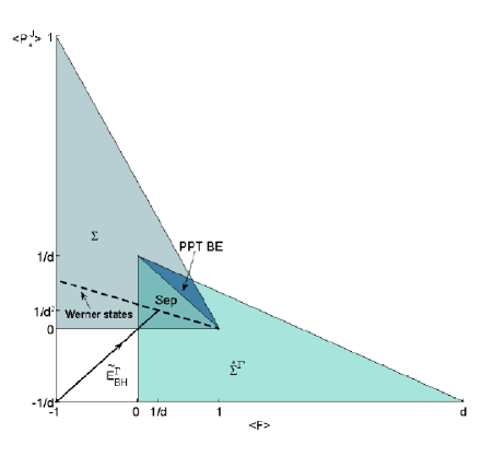
Figure 1: The plot of the set $\Sigma$ of $SS$-invariant states together with $\hat{\Sigma}^{\Gamma}$—the set of partial transposes of $S\bar{S}$-invariant states. The thick line with the arrow represents the partially transposed witness $\widetilde{E}_{BH}^{\Gamma}(p)$. The dashed line represents Werner states; its prolongation to the vertex $(d,-1/d)\equiv\hat{\Pi}_{0}^{\Gamma}$ gives NPT isotropic states. The family $\rho(\lambda)$ from Ref. Breuer is given by the edge, connecting vertices $(-1,1)\equiv\Pi_{0}$ and $(1,0)\equiv\Pi_{2}$. The plot of $\hat{\Sigma}$, $\Sigma^{\Gamma}$, and $\widetilde{E}_{BH}(p)$ is identical, with the axes labels changed to $\langle\bm{F}^{J}\rangle$ and $\langle P_{+}\rangle$ respectively.

The intersection $\hat{\Sigma}^{\Gamma}\cap\Sigma$ describes those $S\bar{S}$-invariant states with positive partial transpose. As shown in Appendix C, not all of them are separable, i.e. there are PPT entangled states in the family. The extreme points of the intersection are given by:

$$x_{0} = (0,0),\ x_{1}=\left(0,\frac{1}{d}\right),$$

$$x_{2} = (1,0),\ x_{3}=\left(\frac{d}{d+2},\frac{1}{d+2}\right).$$ (66)

To prove separability of a given point it is enough to show that there exists a normalized product vector $|u\rangle\otimes|v\rangle$ with the identical expectation values of $\bm{F}$ and $P_{+}^{J}$, for the latter values characterize the state uniquely. Using this fact, one can see that the extreme points of the separability region are $x_{0}$, $x_{1}$ and $x_{2}$. The remaining part of the PPT region contains entangled states.

IV.3.2 Entanglement breaking property of $\widetilde{\Lambda}_{BH}$

We can now return to the study of the witness $\widetilde{E}_{BH}$ associated with the Breuer-Hall map (cf. Eq. (50) with $U=J$). As we have shown in Section IV.3, $\widetilde{E}_{BH}$ is a $S\bar{S}$-invariant hermitean operator. Before analyzing when it becomes positive, note that:

$$\widetilde{E}_{BH}^{\Gamma} = \frac{1}{d-2}\bigg{[}\frac{d-2p}{d^{2}}{\bf 1}-\frac{1-p}{d}\bm{F}-(1-p)P_{+}^{J}\bigg{]}$$ (67)

$$= \big{(}{\bf 1}\otimes J\big{)}\widetilde{E}_{BH}\big{(}{\bf 1}\otimes J^{\dagger}\big{)}.$$

Thus, $\widetilde{E}_{BH}\geq 0$ if and only if $\widetilde{E}_{BH}^{\Gamma}\geq 0$, i.e. the structural-approximated witness is a PPT state.

From Eqs.(50) and (67) we obtain that when $0\leq p\leq 1$:

$$-1\leq\text{tr}(\widetilde{E}_{BH}\bm{F}^{J})=\text{tr}(\widetilde{E}_{BH}^{\Gamma}\bm{F})\leq\frac{1}{d},$$ (68)

$$-\frac{1}{d}\leq\text{tr}(\widetilde{E}_{BH}P_{+})=\text{tr}(\widetilde{E}_{BH}^{\Gamma}P_{+}^{J})\leq\frac{1}{d^{2}}.$$ (69)

The corresponding interval $p\mapsto\widetilde{E}_{BH}^{\Gamma}(p)$ is depicted in Fig. 1 by the thick line with the arrow. We have plotted $\widetilde{E}_{BH}^{\Gamma}(p)$ rather than $\widetilde{E}_{BH}(p)$. One sees that the line enters the positive region $\Sigma$ at the point $x_{0}=(0,0)$, that is when both averages (68) and (69) vanish. Equating any of the expectation values to zero gives the condition for the structural physical approximation:

$$p\geq\frac{d}{d+1}.$$ (70)

Notice that it is the same bound as in Eq. (38) for the reduction map. Observing Fig. 1 it is clear that any structural approximation to Breuer-Hall map is entanglement breaking since the positivity region of $\widetilde{E}_{BH}^{\Gamma}$ is inside the separability region of SS-invariant states.

As a byproduct, we also obtain the minimum eigenvalue $\lambda_{min}$ of the witness $E_{BH}$, corresponding to the original positive map (49). From Eq. (8) it follows that at the critical probability $p=d/(d+1)$ one must have $p/d^{2}+(1-p)\lambda_{min}=0$. This leads to $\lambda_{min}=-1/d$, which corresponds to the eigenvector $|\Phi_{+}\rangle$. Note that this eigenvector shares the symmetry of $E_{BH}$: $S\otimes\bar{S}|\Phi_{+}\rangle=|\Phi_{+}\rangle$.

Again, we are able to provide a representation of the structural approximation to Breuer-Hall map using the $S\bar{S}$-invariance of the corresponding witness:

$$\widetilde{E}_{BH}=\int\text{d}S(S\otimes\bar{S})|\varphi\rangle\langle\varphi|(S\otimes\bar{S})^{{\dagger}}.$$ (71)

These states are parameterized by $\langle P_{+}\rangle$ and $\langle\bm{F}^{J}\rangle$ and, for the critical witness $\widetilde{E}_{BH}$ we have $\langle P_{+}\rangle=\langle\bm{F}^{J}\rangle=0$. The same expected values are obtained by the separable state $|\varphi\rangle=|\phi\rangle\otimes|\psi\rangle$, where

$$|\phi\rangle = \frac{1}{2}\left(|0\rangle+|1\rangle+|2\rangle+|3\rangle\right)$$ (72)

$$|\psi\rangle = \frac{1}{\sqrt{2}}\left(|0\rangle-|2\rangle\right).$$ (73)

Then, the Holevo form of $\widetilde{\Lambda}_{BH}$ is:

$$\widetilde{\Lambda}_{BH}(\varrho)=\int\text{d}S|w_{S}\rangle\langle w_{S}|\text{tr}\left(d|v_{S}\rangle\langle v_{S}|\varrho\right)$$ (74)

with $|v_{S}\rangle=S|\phi\rangle$ and $|w_{S}\rangle=S|\bar{\psi}\rangle$.

V Entanglement Detection via Structural Approximations

Before concluding, we would like to discuss the application of these ideas to the design of entanglement detection methods. Indeed, one of the main motivations for the introduction of structural approximations pawel_ekert was to obtain approximate physical realizations of positive maps, which can then be used for experimental entanglement detection.

The original scheme proposed in pawel_ekert works as follows, see also Fig. 2. Given $N$ copies of an unknown bipartite state, $\varrho_{AB}$, the goal is to determine, without resorting to full tomography, whether the state is PPT. The idea is to apply the structural approximation to partial transposition to this initial state and estimate the spectrum (or more precisely, the minimal eigenvalue) of the resulting state using the optimal measurement for spectrum estimation described in spectrest . Note that the structural approximation $\widetilde{{\bf 1}\otimes T}$ “simply” adds white noise to the ideal operator $\varrho^{\Gamma}$. Thus, it is immediate to relate the spectrum of $(\widetilde{{\bf 1}\otimes T})(\varrho_{AB})$ to the positivity of the partial transposition of the initial state.

Inspired by the previous findings, we study in this section whether the structural approximation to partial transposition defines an entanglement breaking channel. This map is of course not even positive (so it does not entirely fit with our main considered scenario), but obviously by adding sufficient amount of noise it can be made not only positive but also completely positive. As we show next, the structural approximation to partial transposition does indeed define an entanglement breaking channel whenever $d_{A}\geq d_{B}$, which includes the most relevant case of equal dimension $d_{A}=d_{B}$.

This implies that the entanglement detection scheme of Fig. 2.a can just be replaced by a sequence of single-copy measurements, see Fig. 2.b, being the measurement the one associated to the Holevo form of the entanglement breaking channel. This alternative scheme is much simpler from an implementation point of view since it does not require any collective measurement, though the measurements are not projective. Moreover, it can never be worse than the previous method, and most likely is better (see also remik ).

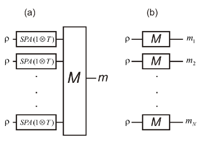
Figure 2: The original scheme for direct entanglement detection proposed in pawel_ekert is shown in (a). Given $N$ copies of an unknown state $\varrho$, it consists of, first, the structural approximation of partial transposition acting on the initial state, followed by optimal estimation of the minimal eigenvalue of the resulting state. In the new scheme, all this structure is replaced by single-copy measurements on the state. The minimal eigenvalue should then be directly estimated from the obtained outcomes.

V.1 Structural Approximations to ${\bf 1}\otimes T$

Let us then consider the structural approximation to transposition extended to some arbitrary auxiliary space: ${\bf 1}_{A}\otimes T_{B}$ pawel_ekert . Note that, unlike in the previous cases, the initial Hilbert space describing the system is now explicitly a product $\mathcal{H}=\mathcal{H}_{A}\otimes\mathcal{H}_{B}\cong\mathbb{C}^{d_{A}}\otimes\mathbb{C}^{d_{B}}$. Moreover, generally $\widetilde{{\bf 1}\otimes\Lambda}$ is not the same as ${\bf 1}\otimes\widetilde{\Lambda}$, although $\widetilde{{\bf 1}\otimes\Lambda}(P_{+})={\bf 1}\otimes\widetilde{\Lambda}(P_{+})$, so this problem does not reduce to the previous one. Calculating the witness corresponding to $\widetilde{{\bf 1}_{A}\otimes T_{B}}$ one obtains:

$$\widetilde{E}_{{\bf 1}\otimes T}=\big{[}({\bf 1}_{A}\otimes{\bf 1}_{B})\otimes(\widetilde{{\bf 1}_{A^{\prime}}\otimes T_{B^{\prime}}})\big{]}(P_{+}^{AB,A^{\prime}B^{\prime}})$$

$$=\frac{p}{(d_{A}d_{B})^{2}}{\bf 1}_{AA^{\prime}}\otimes{\bf 1}_{BB^{\prime}}+\frac{1-p}{d_{B}}P_{+}^{AA^{\prime}}\otimes\bm{F}^{BB^{\prime}},$$ (75)

where $\bm{F}^{BB^{\prime}}$ is the flip operator on $\mathcal{H}_{B}\otimes\mathcal{H}_{B^{\prime}}\cong\mathbb{C}^{d_{B}}\otimes\mathbb{C}^{d_{B}}$ and $P_{+}^{AB,A^{\prime}B^{\prime}}$, $P_{+}^{AA^{\prime}}$ are projectors onto maximally entangled vectors in the corresponding spaces,

$$P_{+}^{AB,A^{\prime}B^{\prime}}=\frac{1}{d_{A}d_{B}}\sum_{i,k=1}^{d_{A}}\sum_{j,l=1}^{d_{B}}|ij\rangle_{AB}\langle kl|\otimes|ij\rangle_{A^{\prime}B^{\prime}}\langle kl|.$$ (76)

The condition for structural approximation, positivity of $\widetilde{E}_{{\bf 1}\otimes T}$, is most easily derived by using the identity $\bm{F}^{BB^{\prime}}=\Pi^{BB^{\prime}}_{+}-\Pi^{BB^{\prime}}_{-}$, where $\Pi^{BB^{\prime}}_{+}$ is the projector on the symmetric subspace $\text{Sym}(\mathcal{H}_{B}\otimes\mathcal{H}_{B^{\prime}})$, and introducing a projector $Q_{+}^{AA^{\prime}}={\bf 1}_{AA^{\prime}}-P_{+}^{AA^{\prime}}$. Then $\widetilde{E}_{{\bf 1}\otimes T}$ becomes:

$$\widetilde{E}_{{\bf 1}\otimes T} = \bigg{[}\frac{p}{(d_{A}d_{B})^{2}}+\frac{1-p}{d_{B}}\bigg{]}P_{+}^{AA^{\prime}}\otimes\Pi^{BB^{\prime}}_{+}$$ (77)

$$+ \frac{p}{(d_{A}d_{B})^{2}}\Big{[}Q_{+}^{AA^{\prime}}\otimes\Pi^{BB^{\prime}}_{+}+Q_{+}^{AA^{\prime}}\otimes\Pi^{BB^{\prime}}_{-}\Big{]}$$

$$+ \bigg{[}\frac{p}{(d_{A}d_{B})^{2}}-\frac{1-p}{d_{B}}\bigg{]}P_{+}^{AA^{\prime}}\otimes\Pi^{BB^{\prime}}_{-}.$$

Since only the last term can be negative, one obtains the following condition for structural approximation:

$$p\geq\frac{d_{A}^{2}d_{B}}{d_{A}^{2}d_{B}+1}.$$ (78)

Comparison of the above threshold with the one given by Eq. (31) with $d=d_{B}$, shows that in order to make ${\bf 1}_{A}\otimes T_{B}$ completely positive one has to add more noise than to make the transposition $T$ alone completely positive and hence implementable. In other words, ${\bf 1}_{A}\otimes\widetilde{T}_{B}$ is less noisy than $\widetilde{{\bf 1}_{A}\otimes T_{B}}$.

We proceed to study the separability of $\widetilde{E}_{{\bf 1}\otimes T}$. We begin by finding the partial transposition of $\widetilde{E}_{{\bf 1}\otimes T}$ with respect to the subsystem $A^{\prime}B^{\prime}$ note0 :

$$\widetilde{E}_{{\bf 1}\otimes T}^{T_{A^{\prime}B^{\prime}}}=\frac{p}{(d_{A}d_{B})^{2}}{\bf 1}+\frac{1-p}{d_{A}}\bm{F}^{AA^{\prime}}\otimes P_{+}^{BB^{\prime}}.$$ (79)

Applying the same technique as above (cf. Eq. (77)), we find that $\widetilde{E}_{{\bf 1}\otimes T}^{\Gamma}\geq 0$ if and only if:

$$p\geq\frac{d_{A}d_{B}^{2}}{d_{A}d_{B}^{2}+1}.$$ (80)

Comparing this to the threshold for positivity (78), we see that for $d_{A}<d_{B}$, i.e. when the extension is by a space of smaller dimension, there is a gap between positivity and PPT. Hence, in this case, for

$$\frac{d_{A}^{2}d_{B}}{d_{A}^{2}d_{B}+1}\leq p\leq\frac{d_{A}d_{B}^{2}}{d_{A}d_{B}^{2}+1}$$ (81)

the witness (77) is not separable and the map $\widetilde{{\bf 1}_{A}\otimes T_{B}}$ is not entanglement breaking in this region. Recall however that this does not represent any counter-example to the conjecture as the initial map is not even positive.

In the case $d_{A}\geq d_{B}$, we will use symmetry arguments to prove the separability of $\widetilde{E}_{{\bf 1}\otimes T}$. From Eq. (75) it follows that this state is $U\bar{U}VV$-invariant, where $U\in U(d_{A})$, $V\in U(d_{B})$ (cf. Refs. werner_sym ; masanes where $UUVV$-invariant states were studied). Since both groups $U(d_{A})$ and $U(d_{B})$ act independently it is easy to convince oneself werner_sym that the space of $U\bar{U}VV$-invariant operators is spanned by $\{{\bf 1}\otimes{\bf 1}$, ${\bf 1}\otimes\bm{F}$, $P_{+}\otimes{\bf 1}$, $P_{+}\otimes\bm{F}$}. Following the same approach as in subsection 121, we prove the separability of $\widetilde{E}_{{\bf 1}\otimes T}$ in the $AB:A^{\prime}B^{\prime}$ partition by showing that the state can be written as convex sum of product states, i.e. it is has the following representation

$$\int\text{d}U\text{d}V(U_{A}V_{B}\bar{U}_{A^{\prime}}V_{B^{\prime}})\sigma(U_{A}V_{B}\bar{U}_{A^{\prime}}V_{B^{\prime}})^{{\dagger}}$$ (82)

(we omit tensor product signs here for brevity) for some $\sigma$ separable in the partition $AB:A^{\prime}B^{\prime}$. Given that states with this invariance are completely described by parameters $\langle{\bf 1}\otimes\bm{F}\rangle$, $\langle P_{+}\otimes{\bf 1}\rangle$ and $\langle P_{+}\otimes\bm{F}\rangle$, $\sigma$ must obey the conditions: $\text{tr}(\sigma{\bf 1}\otimes\bm{F})=\text{tr}(\widetilde{E}_{{\bf 1}\otimes T}{\bf 1}\otimes\bm{F})$, $\text{tr}(\sigma P_{+}\otimes{\bf 1})=\text{tr}(\widetilde{E}_{{\bf 1}\otimes T}P_{+}\otimes{\bf 1})$ and $\text{tr}(\sigma P_{+}\otimes\bm{F})=\text{tr}(\widetilde{E}_{{\bf 1}\otimes T}P_{+}\otimes\bm{F})$. Such state $\sigma\equiv|\varphi\rangle\langle\varphi|$ can be written as

$$|\varphi\rangle \equiv |\phi\rangle_{AB}\otimes|\psi\rangle_{A^{\prime}B^{\prime}}$$ (83)

$$= \left(\sqrt{\alpha_{00}}|00\rangle+\sqrt{\alpha_{01}}|01\rangle+\sqrt{\alpha_{11}}|11\rangle\right)|00\rangle$$

for

$$\alpha_{00} = \frac{d_{B}}{d_{A}d_{B}^{2}+1}(1+d_{A})$$ (84)

$$\alpha_{01} = \frac{1}{d_{A}d_{B}^{2}+1}(d_{B}^{2}+d_{A}-d_{B}(1+d_{A}))$$ (85)

$$\alpha_{11} = 1-\frac{1}{d_{A}d_{B}^{2}+1}(d_{B}^{2}+d_{A}).$$ (86)

Notice that, as expected, $\sigma$ is only well-defined for $d_{A}\geq d_{B}$. According to Eq. (6), the map $\widetilde{{\bf 1}\otimes T}(\varrho)$ can be written as

$$\widetilde{{\bf 1}\otimes T}(\varrho)=\int\text{d}U\text{d}V|w_{U\bar{V}}\rangle\langle w_{U\bar{V}}|\text{tr}(d_{A}d_{B}|v_{UV}\rangle\langle v_{UV}|\varrho).$$ (87)

where $|v_{UV}\rangle=U\otimes V|\phi\rangle$ and $|w_{U\bar{V}}\rangle=U\otimes\bar{V}|\bar{\psi}\rangle$. Recall also that the integrals over the unitary group defining each depolarization protocol can be replaced by the finite sums of, e.g., Ref. DCLB .

In the case $d_{A}=d_{B}\equiv d$, we encounter the structural approximation to the transposition map analyzed in pawel_ekert . As mentioned, by providing the representation (87) we are able to replace the former entanglement detection scheme pawel_ekert by a much less resource-demanding one. In the original proposal, $n$ copies of $\tilde{T}(\varrho)$ are prepared, followed by optimal estimation of its minimal eigenvalue by means of a collective projective measurement on the $n$-copy state. Now, one should just perform local measurements in the $n$ copies of $\varrho$ with operators defined in (87) and with that directly estimate the lowest eigenvalue of ${\bf 1}\otimes T$.

VI Conclusions

In this work, we have studied the implementation of structural approximations to positive maps via measurement and state-preparation protocols. Our findings suggest an intriguing connection between these two concepts that we have summarized by conjecturing that the structural physical approximation of an optimal positive map defines an entanglement breaking channel. Of course, the main open question is (dis)proving this conjecture. It would also be interesting to obtain slightly weaker results in the same direction, such as proving the conjecture for general optimal decomposable maps (which seems more plausible due to the fact that the conjecture holds for transposition). We have also applied the same ideas to the study of physical approximations to partial transposition, which is not a positive map, and discuss the implications of our results for entanglement detection.

We would like to conclude this work by giving a geometrical representation of our findings (that should be interpreted in an approximate way). It is well known that the set of quantum states is convex and includes the set of separable states, which is also convex, see also Fig. 3. These two sets are contained in the set of Hermitian operators that are positive on product states, which is again convex. Entanglement witnesses belong to this set. If the conjecture was true, it would mean that the set of optimal witnesses would live in a region which is “opposite" to the set of separable states, in the sense that when mixed with the maximally mixed noise, they enter the set of physical states via the separability region.

Finally, let us mention some further open questions. It would be interesting to extend our studies and ask which classes of positive maps have structural approximation that corresponding to partially breaking channels (for definition see darek1 )? Is our conjecture true for maps that are not optimal, but atomic darek2 , i.e. detect Schmidt number 2 entanglement (for definition see SBL ? What is the relation between optimality, extremality (in the sense of convex sets) and atomic property?

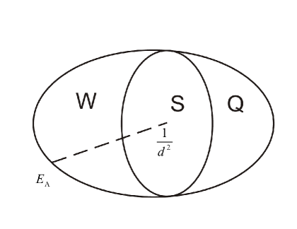
Figure 3: The sets $S$, $Q$ and $W$ of separable states, quantum states and operators positive on product states are such that $S\subset Q\subset W$. If the conjecture was true, namely all structural approximations to optimal positive maps defined entanglement breaking channels, it would mean that optimal positive maps (witnesses) enter the physical region, when adding white noise, via the separability region, as shown in the figure.

Appendix A: Proof of the conjecture for a rank-three optimal witness in $2\otimes 4$ systems

In this appendix, we show that the structural approximation to the optimal witness $Q^{\Gamma}$, where $Q$ is the projector onto states (27), is separable. Following our general procedure (cf. Eq. (8)), the normalized witness associated to the structural approximation reads:

$$\widetilde{E}_{\Lambda}=\frac{p}{8}{\bf 1}+\frac{1-p}{6}Q^{\Gamma}\equiv\frac{1-p}{6}\Big{(}Q^{\Gamma}+a{\bf 1}\Big{)}$$

$$=\frac{1-p}{6}\times$$

$$\left[\begin{array}[]{cccccccc}a&0&0&0&0&-1&0&0\\ 0&1+a&0&0&0&0&-1&0\\ 0&0&1+a&0&0&0&0&-1\\ 0&0&0&1+a&0&0&0&0\\ 0&0&0&0&1+a&0&0&0\\ -1&0&0&0&0&1+a&0&0\\ 0&-1&0&0&0&0&1+a&0\\ 0&0&-1&0&0&0&0&a\end{array}\right],$$ (96)

where $a=\frac{6p}{8(1-p)}$. The above operator becomes positive when

$$a(1+a)=1.$$ (97)

To show that at this point the matrix (96) becomes separable, we first perform a local invertible transformation and pass from $Q^{\Gamma}+a{\bf 1}$ to ${\bf 1}\otimes A\Big{(}Q^{\Gamma}+a{\bf 1}\Big{)}{\bf 1}\otimes A^{\dagger}$, where

$$A=\left[\begin{array}[]{cccc}1&0&0&0\\ 0&a&0&0\\ 0&0&a&0\\ 0&0&0&1\end{array}\right].$$ (98)

With the help of the positivity condition (97), the resulting matrix can be written as:

$$a^{2}\left[\begin{array}[]{cccccccc}1&0&0&0&0&-1&0&0\\ 0&1&0&0&0&0&-1&0\\ 0&0&1&0&0&0&0&-1\\ 0&0&0&1&0&0&0&0\\ 0&0&0&0&1&0&0&0\\ -1&0&0&0&0&1&0&0\\ 0&-1&0&0&0&0&1&0\\ 0&0&-1&0&0&0&0&1\end{array}\right]+$$ (107)

$$+(a-a^{2})\left[\begin{array}[]{cccccccc}1&0&0&0&0&-1&0&0\\ 0&1&0&0&0&0&0&0\\ 0&0&1&0&0&0&0&-1\\ 0&0&0&\kappa&0&0&0&0\\ 0&0&0&0&\kappa&0&0&0\\ -1&0&0&0&0&1&0&0\\ 0&0&0&0&0&0&1&0\\ 0&0&-1&0&0&0&0&1\end{array}\right],$$ (116)

where

$$\kappa=\frac{1}{a-a^{2}}\Big{(}\frac{1}{a}-a^{2}\Big{)}>1.$$ (117)

Note that since at the critical point (97), $a-a^{2}>0$, it is enough to show that both matrices in the above decomposition are separable. The first matrix, which we denote by $\sigma$, possesses the following continuous separable representation:

$$\sigma=\int_{0}^{2\pi}\frac{\text{d}\phi}{2\pi}|\psi(\phi)\rangle\langle\psi(\phi)|,$$ (118)

where

$$\psi(\phi)=(\text{e}^{\text{i}\phi},-1)\otimes(1,\text{e}^{\text{i}\phi},\text{e}^{2\text{i}\phi},\text{e}^{3\text{i}\phi}).$$ (119)

The second matrix has a $(2\otimes 2)\oplus(2\otimes 2)$ structure with $2\otimes 2$ blocks being identical and given by

$$\left[\begin{array}[]{cccc}1&0&0&-1\\ 0&1&0&0\\ 0&0&\kappa&0\\ -1&0&0&1\end{array}\right].$$ (120)

Since $\kappa>1$ the above matrix is PPT and hence separable. Thus, the whole matrix (116) is separable, which finishes the proof.

Appendix B: $3\otimes 3$ systems

In this appendix, we provide several examples of positive maps satisfying the conjecture. Again we consider decomposable optimal maps and study case-by-case various possible ranks of the $Q$ operator (cf. Theorem 2, Section II.2).

The case $r(Q)=1$, i.e. $Q=|\psi\rangle\langle\psi|$, splits into two subcases. When the Schmidt-rank of $|\psi\rangle$ is 2, $Q$ is supported in a $2\otimes 2$ subspace and the structural approximation is entanglement breaking by the previous results (cf. Section III.1). In the case where $|\psi\rangle$ is Schmidt-rank 3, we restrict our attention to the trace-preserving case, i.e. assume that $|\psi\rangle$ is maximally entangled. Alternatively, before checking the conjecture we apply local transformations and bring $|\psi\rangle$ to the form (2), i.e. we assume that:

$$|\psi\rangle=\frac{1}{\sqrt{3}}\Big{(}|00\rangle+|11\rangle+|22\rangle\Big{)}=|\Phi_{+}\rangle.$$ (121)

Then the corresponding witness $\tilde{E}$ from Eq. (8) turns out to be a Werner state Werner of dimension $d=3$. This witness was already studied for arbitrary $d$ in section , where we concluded that such structural approximation is always entanglement breaking.

We move to the case $r(Q)=2$. Then $Q$ has to be supported either in a $2\otimes 3$ subspace or in the full $3\otimes 3$ space, since in $2\otimes 2$ there is always a product vector in every two dimensional subspace and $Q$ would not be optimal by Theorem 2 of Section II.2. The first case, when $Q$ is supported in a $2\otimes 3$ subspace, is covered by Section III.1. In the other case, we do not have a general theory, but in a generic case the range of $Q$ is spanned by two Schmidt-rank 2 vectors. We can take them to be:

$$|01\rangle-|10\rangle$$ (122)

$$|12\rangle-|21\rangle.$$ (123)

Obviously, for such a $Q$ it holds $Qe\otimes e=0\Rightarrow\langle e\otimes\bar{e}|Q^{\Gamma}e\otimes\bar{e}\rangle=0$ for any $e\in\mathbb{C}^{3}$. Since vectors $e\otimes\bar{e}$ span the whole $\mathbb{C}^{3}\otimes\mathbb{C}^{3}$, by Corollary 2 of Section II.1 the witness $Q^{\Gamma}$ is optimal.

Again we do not have a general result here, but only consider a generic example of $Q$ given by the projectors on the above vectors (122-123). The normalized witness corresponding to the structural approximation, $\widetilde{E}_{\Lambda}=\frac{1-p}{4}\Big{(}Q^{\Gamma}+a{\bf 1}\Big{)}$ with $a=\frac{4p}{9(1-p)}$ is given, modulo the $(1-p)/4$ prefactor, by the matrix:

$$\left[\begin{array}[]{ccccccccc}a&0&0&0&-1&0&0&0&0\\ 0&1+a&0&0&0&0&0&0&0\\ 0&0&a&0&0&0&0&0&0\\ 0&0&0&1+a&0&0&0&0&0\\ -1&0&0&0&a&0&0&0&-1\\ 0&0&0&0&0&1+a&0&0&0\\ 0&0&0&0&0&0&a&0&0\\ 0&0&0&0&0&0&0&1+a&0\\ 0&0&0&0&-1&0&0&0&a\end{array}\right].$$ (124)

It becomes positive at the point $a(a^{2}-2)=0$, i.e. at

$$a=\sqrt{2}.$$ (125)

which gives the critical probability $p_{c}=\frac{9\sqrt{2}}{9\sqrt{2}+1}\approx 0.93.$

To check the separability at the above point (125), note that the matrix (124) can be decomposed as follows:

$$\left[\begin{array}[]{ccccccccc}a&0&0&0&-1&0&0&0&0\\ 0&1+a&0&0&0&0&0&0&0\\ 0&0&0&0&0&0&0&0&0\\ 0&0&0&1+a&0&0&0&0&0\\ -1&0&0&0&\frac{a}{2}&0&0&0&0\\ 0&0&0&0&0&0&0&0&0\\ 0&0&0&0&0&0&0&0&0\\ 0&0&0&0&0&0&0&0&0\\ 0&0&0&0&0&0&0&0&0\end{array}\right]+$$ (135)

$$+\left[\begin{array}[]{ccccccccc}0&0&0&0&0&0&0&0&0\\ 0&0&0&0&0&0&0&0&0\\ 0&0&0&0&0&0&0&0&0\\ 0&0&0&0&0&0&0&0&0\\ 0&0&0&0&\frac{a}{2}&0&0&0&-1\\ 0&0&0&0&0&1+a&0&0&0\\ 0&0&0&0&0&0&0&0&0\\ 0&0&0&0&0&0&0&1+a&0\\ 0&0&0&0&-1&0&0&0&a\end{array}\right]+$$ (145)

$$+\left[\begin{array}[]{ccccccccc}0&0&0&0&0&0&0&0&0\\ 0&0&0&0&0&0&0&0&0\\ 0&0&a&0&0&0&0&0&0\\ 0&0&0&0&0&0&0&0&0\\ 0&0&0&0&0&0&0&0&0\\ 0&0&0&0&0&0&0&0&0\\ 0&0&0&0&0&0&a&0&0\\ 0&0&0&0&0&0&0&0&0\\ 0&0&0&0&0&0&0&0&0\end{array}\right].$$ (155)

The first two matrices are supported in $2\otimes 2$ subspaces. Their partial transposes become positive for $(1+a)^{2}=1$, which is satisfied at the point (125). The last matrix is obviously separable. This allows us to conclude that the structural approximation (124) is entanglement breaking.

Next, we consider the case $r(Q)=3$. Then $Q$ must be supported in the whole $3\otimes 3$ space (otherwise there would be a product vector in the range of $Q$ and $Q$ would not be optimal by Theorem 2, Section II.2). In lieu of a general theory, we consider a seemingly generic example of

$$Q=\Pi_{-},$$ (156)

where by $\Pi_{\pm}$ we denote the projectors onto the symmetric $\text{Sym}(\mathcal{H}\otimes\mathcal{H})$ and skew-symmetric $\mathcal{H}\wedge\mathcal{H}$ subspaces respectively. The corresponding normalized witness reads:

$$\frac{3}{1-p}\widetilde{E}_{\Lambda}=Q^{\Gamma}+a{\bf 1}=\frac{1}{2}\Big{[}(1+2a){\bf 1}-3P_{+}\Big{]},$$ (157)

where $a=\frac{3p}{9(1-p)}$ and we used the identities $\bm{F}=\Pi_{+}-\Pi_{-}=1-2\Pi_{-}$ and $\bm{F}^{\Gamma}=dP_{+}$. The condition for structural approximation, $\widetilde{E}_{\Lambda}\geq 0$, is equivalent to

$$a\geq 1.$$ (158)

Note that the structural-approximated witness (157) is an isotropic state of dimension $d=3$ and that this was already studied for arbitrary $d$ in Sec. III.4. There we concluded that such witnesses always correspond to entanglement-breaking channels.

We are left with the last case $r(Q)=4$. Note that generically if we consider $P$ a projector on the kernel of $Q$, then $r(P)=5$ and the range of $P$ contains exactly $\leq$ 5 product vectors. In general, $Q$ will contain some product vector in its kernel and therefore is not optimal. For this reason, here we consider not a generic but a particular $Q$ where optimality is guaranteed by the Corollary 2 of Section II.1. We can treat $\mathbb{C}^{3}\otimes\mathbb{C}^{3}$ as a representation space of two spin-$1$ representations of $SU(2)$. We then consider positive operators $Q$ supported on a span of the skew-symmetric subspace $\mathbb{C}^{3}\wedge\mathbb{C}^{3}$ and the singlet Breuer2 :

$$\Psi=\frac{1}{\sqrt{3}}\Big{(}|02\rangle+|20\rangle-|11\rangle\Big{)}.$$ (159)

Denoting by $J$ the total spin, $Q$ is supported on the sum of $J=0$ and $J=1$ subspaces, while $P$ is supported on the $J=2$ subspace. The kernel of $Q$ is then spanned by the vectors of the form $(1,\sqrt{2}\alpha,\alpha^{2})\otimes(1,\sqrt{2}\alpha,\alpha^{2})$ for a complex $\alpha$. By Corollary 2 of Section II.1, $Q^{\Gamma}$ is optimal, as vectors $(1,\sqrt{2}\alpha,\alpha^{2})\otimes(1,\sqrt{2}\bar{\alpha},\bar{\alpha}^{2})$ span whole of the $\mathbb{C}^{3}\otimes\mathbb{C}^{3}$.

As a particular example we consider

$$Q=2\Pi_{-}+2P_{\Psi}.$$ (160)

The structural approximation gives:

$$\frac{8}{1-p}\widetilde{E}_{\Lambda}=Q^{\Gamma}+a{\bf 1}=$$

$$\left[\begin{array}[]{ccccccccc}a&0&0&0&-1&0&0&0&-\frac{1}{3}\\ 0&1+a&0&0&0&-\frac{2}{3}&0&0&0\\ 0&0&\frac{5}{3}+a&0&0&0&0&0&0\\ 0&0&0&1+a&0&0&0&-\frac{2}{3}&0\\ -1&0&0&0&\frac{2}{3}+a&0&0&0&-1\\ 0&-\frac{2}{3}&0&0&0&1+a&0&0&0\\ 0&0&0&0&0&0&\frac{5}{3}+a&0&0\\ 0&0&0&-\frac{2}{3}&0&0&0&1+a&0\\ -\frac{1}{3}&0&0&0&-1&0&0&0&a\end{array}\right],$$ (170)

where

$$a=\frac{8p}{9(1-p)}.$$ (171)

The matrix (170) becomes positive at the point given by the conditions $(a+1)^{2}-\frac{4}{9}=0$ and $\Big{(}a+\frac{2}{3}\Big{)}\Big{(}a-\frac{1}{3}\Big{)}-2=0$, which is solved by

$$a=\frac{4}{3}.$$ (172)

We now prove that at this point the witness (170) becomes separable. We consider the partially transposed witness:

$$\frac{8}{1-p}\widetilde{E}_{\Lambda}^{\Gamma}=\frac{4}{3}{\bf 1}+2\Big{(}P_{J=1}+P_{J=0}\Big{)},$$ (173)

where $P_{J}$ projects on the subspace of total spin $J$. Using the technique based on the state invariance described in Sec. III.3, we explicitly construct a separable decomposition for $\widetilde{E}_{\Lambda}^{\Gamma}$. Analogously to the definition (33), we introduce spin-$1\,\otimes\,$spin-$1$ depolarizing operator:

$$\mathscr{D}(\varrho)=\int\text{d}\mathscr{D}^{(1)}(U)\times$$

$$\big{[}\mathscr{D}^{(1)}(U)\otimes\mathscr{D}^{(1)}(U)\big{]}\varrho\big{[}\mathscr{D}^{(1)}(U)^{\dagger}\otimes\mathscr{D}^{(1)}(U)^{\dagger}\big{]}$$ (174)

$$=\frac{1}{5}\text{tr}\big{(}\varrho P_{J=2}\big{)}P_{J=2}+\frac{1}{3}\text{tr}\big{(}\varrho P_{J=1}\big{)}P_{J=2}+$$

$$+\text{tr}\big{(}\varrho P_{J=0}\big{)}P_{J=0}.$$ (175)

where $\mathscr{D}^{(1)}(U)\in SO(3)$ denotes spin-$1$ representation of $U\in SU(2)$. By direct calculation we check that

$$\mathscr{D}(|02\rangle\langle 02|)+\mathscr{D}(|01\rangle\langle 01|)$$ (176)

gives, up to a positive constant, the desired operator $\widetilde{E}_{\Lambda}^{\Gamma}$. Since separability of $\widetilde{E}_{\Lambda}^{\Gamma}$ is equivalent to separability of $\widetilde{E}_{\Lambda}$, we have thus shown that the structural approximation to the map defined by Eq. (160) is entanglement breaking.

Appendix C: Analysis of Unitary Symplectic Invariant States

The scope of this appendix is to provide a characterization of the properties of $SS$ and $S\bar{S}$ invariant states. The first step is to find the space of Hermitian $SS$-invariant operators. The corresponding space of $S\bar{S}$-invariant ones is related to the latter by partial transposition $\Gamma$. Since unitary symplectic transformations $S$ are obviously unitary, all $UU$-invariant operators are also $SS$-invariant. As it is well known, the former space is spanned by ${\bf 1}$ and $\bm{F}$ Werner . As a rule, shrinking the group enlarges the space of the invariant operators, so one expects more than that. The form of the invariance group $G=Sp(2n,\mathbb{C})\cap U(2n)$ implies that $\{G-\text{inv}\}=\{Sp(2n,\mathbb{C})-\text{inv}\}\cup\{U(2n)-\text{inv}\}$ (in some sense we will not specify here; see Ref. werner_sym ). Thus, one has to find the $Sp(2n,\mathbb{C})$-invariant operators.

Let $A$ be Hermitian and such that:

$$\sum_{j,\dots,n}S_{ij}S_{kl}A_{jlmn}\bar{S}_{rm}\bar{S}_{sn}=A_{ikrs},$$ (177)

for all $S$ from $Sp(2n,\mathbb{C})$ (now $S$ satisfies Eq. (53) only). Since $S$ and its complex conjugation $\bar{S}$ are independent for a general $S\in Sp(2n,\mathbb{C})$, and the defining equation (53) does not involve complex conjugation, the only possibility for Eq. (177) to hold is when $A$ is rank one, i.e. $A_{jlmn}=\psi_{jl}\bar{\phi}_{mn}$. Then Eq. (177) becomes:

$$\big{(}S\psi S^{T}\big{)}_{ik}\overline{\big{(}S\phi S^{T}\big{)}}_{rs}=\psi_{ik}\bar{\phi}_{rs}.$$ (178)

But the only quadratic form that $S$ preserves is $J$, which implies that one must have $\psi_{ik}=c_{1}J_{ik}$ and $\phi_{rs}=c_{2}J_{rs}$ for some complex $c_{1,2}\neq 0$. We choose $c_{1}=c_{2}=-1/\sqrt{d}$, $d=2n$, which leads to:

$$|\psi\rangle = |\phi\rangle=-\frac{1}{\sqrt{d}}\sum_{i,k}J_{ik}|ik\rangle$$ (179)

$$= \frac{1}{\sqrt{d}}\big{(}|10\rangle-|01\rangle+|32\rangle-|23\rangle+\dots\big{)}$$

$$= ({\bf 1}\otimes J)|\Phi_{+}\rangle,$$

(cf. Eq. (2)). Hence, $P_{+}^{J}=({\bf 1}\otimes J)P_{+}({\bf 1}\otimes J^{\dagger})$ is the only $Sp(2n,\mathbb{C})$-invariant operator, up to a multiplicative constant note1 . Using this fact we conclude that the space of $SS$-invariant operators is spanned by $\{{\bf 1},\bm{F},P_{+}^{J}\}$. Correspondingly, the space of $S\bar{S}$-invariant operators is spanned by $\{{\bf 1},\bm{F},P_{+}^{J}\}^{\Gamma}\equiv\{{\bf 1},P_{+},\bm{F}^{J}\}=({\bf 1}\otimes J)\{{\bf 1},P_{+}^{J},\bm{F}^{J}\}({\bf 1}\otimes J^{\dagger})$. As a side remark, we note that since $J$ is real, $J^{\dagger}=J^{T}=-J$ (cf. definition (51)) and hence $({\bf 1}\otimes J)A({\bf 1}\otimes J^{\dagger})=-({\bf 1}\otimes J)A({\bf 1}\otimes J)$ for any $A$. We will use this fact frequently, but keep writing $J^{\dagger}$.

As a general rule, $G$-invariant operators form algebras werner_sym . The constituent relations for the algebras of unitary symplectic invariant operators are as follows:

$$\bm{F}P_{+}^{J} = -P_{+}^{J}=P_{+}^{J}\bm{F}\quad$$

and

$$\quad P_{+}\bm{F}^{J} = -P_{+}=\bm{F}^{J}P_{+}.$$ (181)

The above relations follow from the identity $\bm{F}({\bf 1}\otimes J)|\Phi_{+}\rangle=(J\otimes{\bf 1})|\Phi_{+}\rangle=-({\bf 1}\otimes J)|\Phi_{+}\rangle$, equivalent to $\bm{F}^{J}|\Phi_{+}\rangle=-|\Phi_{+}\rangle$.

Let us now focus on the study of the PPT region, resulting from the intersection $\hat{\Sigma}^{\Gamma}\cap\Sigma$. As we mentioned, when studying separability, one should characterize the expectation value of the generators of the group with product vectors. For a vector $|u\rangle\otimes|v\rangle$ one obtains that:

$$\langle\bm{F}\rangle =\big{|}\langle u|v\rangle\big{|}^{2}$$

$$= \big{|}\bar{u}_{0}v_{0}+\bar{u}_{1}v_{1}+\bar{u}_{2}v_{2}+\bar{u}_{3}v_{3}+\dots+\bar{u}_{2n}v_{2n}\big{|}^{2},$$

$$\langle P_{+}^{J}\rangle =\frac{1}{d}\big{|}u^{T}Jv\big{|}^{2}$$

$$= \frac{1}{d}\big{|}u_{0}v_{1}-u_{1}v_{0}+\dots+u_{2n-1}v_{2n}-u_{2n}v_{2n-1}\big{|}^{2}.$$

(182)

From these equations, one easily sees that the first extreme point from (IV.3.1) can be realized by e.g. $u=(1/2)(-1,1,1,1,0,\dots)$ and $v=1/\sqrt{2}(1,0,0,1,0,\dots)$, while points $x_{2},x_{3}$ can be obtained from $u=1/\sqrt{2}\big{(}|0\rangle\mp|1\rangle\big{)}$, $v=1/\sqrt{2}\big{(}|0\rangle+|1\rangle\big{)}$ respectively. To show that only the set $\text{conv}\{x_{0},x_{1},x_{2}\}$ is separable we will employ the Breuer-Hall map (49) itself. Note that the corresponding separable set $\text{conv}\{x_{0},x_{1},x_{2}\}^{\Gamma}\subset\hat{\Sigma}\cap\Sigma^{\Gamma}$ is determined by the points with the same coordinates as $x_{0},x_{1},x_{2}$ but in the $\langle P_{+}\rangle,\langle\bm{F}^{J}\rangle$-plane (since e.g. $\text{tr}(\varrho^{\Gamma}P_{+}^{J})=1/d$ $\Leftrightarrow$$\text{tr}(\varrho\bm{F})=1$, etc).

For an arbitrary $SS$-invariant normalized state $\varrho=\alpha{\bf 1}+\beta\bm{F}+\gamma P_{+}^{J}$ it holds $\text{tr}_{B}\varrho=\big{(}d\alpha+\bm{F}+(1/d)\gamma\big{)}{\bf 1}={\bf 1}/d$, since $\text{tr}\varrho=d^{2}\alpha+d\beta+\gamma=1$ and $\text{tr}_{B}P_{+}^{J}=\text{tr}_{B}P_{+}={\bf 1}/d$ as $J$ is unitary. Analogously, for an arbitrary $S\bar{S}$-invariant state $\hat{\varrho}=\hat{\alpha}{\bf 1}+\hat{\beta}\bm{F}^{J}+\hat{\gamma}P_{+}$, $\text{tr}_{B}\hat{\varrho}={\bf 1}/d$, since $\text{tr}_{B}\bm{F}^{J}=\text{tr}_{B}\bm{F}={\bf 1}$. Hence, the no-detection condition ${\bf 1}\otimes\Lambda_{BH}(\varrho)\geq 0$ takes the same form for both families:

$$\frac{1}{d}{\bf 1}-\varrho-\big{(}{\bf 1}\otimes J\big{)}\varrho^{\Gamma}\big{(}{\bf 1}\otimes J^{\dagger}\big{)}\geq 0.$$ (183)

We multiply the above inequality by $P_{+}^{J}$ and $P_{+}$ respectively. Noting that $P_{+}^{J},P_{+}\geq 0$ and $[{\bf 1}\otimes\Lambda_{BH}(\varrho),P_{+}^{J}]=0=[{\bf 1}\otimes\Lambda_{BH}(\hat{\varrho}),P_{+}]$, we obtain that if a state is not detected by the Breuer-Hall map then:

$$\text{tr}(\varrho P_{+}^{J})\leq\frac{1-\text{tr}(\varrho\bm{F})}{d},\quad\text{or}$$ (184)

$$\text{tr}(\hat{\varrho}P_{+})\leq\frac{1-\text{tr}(\hat{\varrho}\bm{F}^{J})}{d}$$ (185)

respectively. Equivalently, states breaking the above inequalities, i.e. states lying above the line $\langle P_{+}^{J}\rangle=\big{(}1-\langle\bm{F}\rangle\big{)}/d$, or above the line $\langle P_{+}\rangle=\big{(}1-\langle\bm{F}^{J}\rangle\big{)}/d$ in the case of $S\bar{S}$-invariant states, are detected by $\Lambda_{BH}$ and hence entangled.

The set of PPT entangled $S\bar{S}$-invariant states is depicted in Fig. 1. Note that when $d\to\infty$, $d$ even, the point $x_{3}\to x_{2}$, cf. Eq. (IV.3.1), and the set of PPT bound entangled states collapses. Since we expect that away from region boundaries in Fig. 1 the properties of $S\bar{S}$-invariant states are shared by the states in a small ball around them, the collapse of the "volume" of the PPT states is to be expected according to Ref. PPTBEinf . From the previous arguments (cf. remarks after Eq. (65)) and Eq. (185), the corresponding diagram for $SS$-invariant states is identical, modulo the labels of the axes. This finishes our analysis of unitary symplectic invariant states.

References

- (1) R. Horodecki, P. Horodecki, M. Horodecki, and K. Horodecki, Rev. Mod. Phys., in press; arXiv:quant-ph/0702225v2.
- (2) A. G. White, J. R. Mitchell, O. Nairz, and P. G. Kwiat, Phys. Rev. A 58, 605 (1998).
- (3) H. Häffner, W. Hänsel, C. F. Roos, J. Benhelm, D. Chek-al-kar, M. Chwalla, T. Korber, U. D. Rapol, M. Riebe, P. O. Schmidt, C. Becher, O. Gühne, W. Dür, and R. Blatt, Nature 438, 643 (2005).
- (4) J. K. Korbicz, O. Gühne, M. Lewenstein, H. Häffner, C. F. Roos, and R. Blatt, Phys. Rev. A 74, 052319 (2006).
- (5) G. Jaeger, M. A. Horne, and Abner Shimony, Phys. Rev. A 48, 1023 (1993); H. Weinfurter, and Żukowski Phys. Rev. A 64, 010102 (2001).
- (6) J. S. Bell, Speakable and Unspeakable in Quantum Mechamics, (Cambridge University Press, Cambridge, 2004); J. F. Clauser, M. A. Horne, A. Shimony, and R. A. Holt, Phys. Rev. Lett. 23, 880 (1969).
- (7) R. F. Werner, Phys. Rev. A 40, 4277 (1989).
- (8) J. Barrett Phys. Rev. A 65, 042302 (2002); G. Tóth and A. Acín, Phys. Rev. A 74, 030306 (2006); M. L. Almeida, S. Pironio, J. Barrett, G. Tóth, and A. Acín, Phys. Rev. Lett. 99, 040403 (2007).
- (9) R. F. Werner and M. Wolf, Quant. Inform. and Comp. 1, 1 (2001).
- (10) M. Horodecki, P. Horodecki, and R. Horodecki, Phys. Lett. A 223, 1 (1996).
- (11) B. M. Terhal, Phys. Lett. A 271, 319 (2000).
- (12) J. M. Sancho and S. F. Huelga, Phys. Rev. A 61, 042303 (2000); A. Acín, R. Tarrach and G. Vidal, Phys. Rev. A 61, 062307 (2000).
- (13) L. Aolita and F. Mintert, Phys. Rev. Lett. 97, 050501 (2006); F. Mintert and A. Buchleitner, Phys. Rev. Lett. 98, 140505 (2007).
- (14) P. Horodecki, Phys. Rev. A 68, 052101 (2003).
- (15) P. Horodecki and A. Ekert, Phys. Rev. Lett. 89, 127902 (2002).
- (16) O. Gühne and N. Lütkenhaus, Phys. Rev. Lett. 96, 170502 (2006).
- (17) O. Gühne, Phys. Rev. Lett. 92, 117903 (2004); G. Tóth, C. Knapp, O. Gühne, and H. J. Briegel, Phys. Rev. Lett. 99, 250405 (2007).
- (18) J. K. Korbicz, J. I. Cirac, and M. Lewenstein, Phys. Rev. Lett. 95, 120502 (2005); Erratum ibid. 95, 259901 (2005).
- (19) O. Gühne and M. Lewenstein, Phys. Rev. A 70, 022316 (2004).
- (20) O. Gühne, P. Hyllus, D. Bruss, A. Ekert, M. Lewenstein, C. Macchiavello, and A. Sanpera, Phys. Rev. A 66, 062305 (2002).
- (21) M. Barbieri, F. De Martini, G. Di Nepi, P. Mataloni, G. M. D’Ariano, and C. Macchiavello, Phys. Rev. Lett. 91, 227901 (2003).
- (22) M. Bourennane, M. Eibl, C. Kurtsiefer, S. Gaertner, H. Weinfurter, O. Gühne, P. Hyllus, D. Bruss, M. Lewenstein, and A. Sanpera, Phys. Rev. Lett. 92, 087902 (2004).
- (23) K. Kraus, States, Effects, and Operators: Fundamental Notions of Quantum Theory (Springer, Berlin, 1983).
- (24) S. L. Woronowicz, Rep. Math. Phys. 10, 165 (1976); Comm. Math. Phys. 51, 243 (1976); P. Kruszyński and S. L. Woronowicz, Lett. Math. Phys. 3, 317 (1979).
- (25) A. Peres, Phys. Rev. Lett. 77, 1413 (1996).
- (26) P. Horodecki, Phys. Lett. A 232, 333 (1997).
- (27) Throughout this paper, and for the sake of simplicity, we often name as positive maps those maps that are positive but not completely positive.
- (28) A. Jamiołkowski, Rep. Math. Phys. 3, 275 (1972); M.-D. Choi, Linear Algebra Appl. 10, 285 (1975).
- (29) J. K. Korbicz, J. Wehr, and M. Lewenstein, Comm. Math. Phys. 281, 753 (2008).
- (30) M. Horodecki, P. W. Shor, and M. B. Ruskai, Rev. Math. Phys 15, 629 (2003).
- (31) A. Peres, Quantum Theory: Concepts and Methods, (Kluwer Academic Publishers, Dordrecht, 1993).
- (32) Similar ideas concerning transposition were developed recently by R. Augusiak and J. Stasińska, Phys. Rev. A 77, 010303(R) (2008).
- (33) I. Bengtsson and K. Życzkowski, Geometry of Quantum States: An Introduction to Quantum Entanglement, (Cambridge University Press, Cambridge, 2006).
- (34) M. Lewenstein, B. Kraus, J. I. Cirac, and P. Horodecki, Phys. Rev. A 62, 052310 (2000).
- (35) M. Lewenstein, B. Kraus, J. I. Cirac, and P. Horodecki Phys. Rev. A 63, 044304 (2001).
- (36) C. H. Bennett, D. P. DiVincenzo, T. Mor, P. W. Shor, J. A. Smolin, and B.M. Terhal, Phys. Rev. Lett. 82, 5385 (1999); D. P. DiVincenzo, T. Mor, P. W. Shor, J. A. Smolin, and B. M. Terhal, Comm. Math. Phys. 238, 379 (2003).
- (37) J. Samsonowicz, M. Kuś, and M.Lewenstein, Phys. Rev. A 76, 022314 (2007).
- (38) M. Horodecki and P. Horodecki, Phys. Rev. A 59, 4206 (1999).
- (39) H.-P. Breuer, Phys. Rev. Lett. 97, 080501 (2006).
- (40) W. Hall, J. Phys. A 39, 14119 (2006).
- (41) K. G. H. Vollbrecht and R. F. Werner, Phys. Rev. A 64, 062307 (2001).
- (42) Y.-C. Liang, Ll. Masanes, and A. C. Doherty, Phys. Rev. A 77, 012332 (2008).
- (43) W. Dür, J. I. Cirac, M. Lewenstein and D. Bruss, Phys. Rev. A 61, 062313 (2000).
- (44) M. D. Choi, J. Operator Theory, 4, 271 (1980).
- (45) Observe that and analogously , and .
- (46) H.-P. Breuer, Phys. Rev. A 71, 062330 (2005).
- (47) The other possibilities give nothing new as: and, trivially, .
- (48) For a general unitary symplectic invariant operator , although it can happen (see Eq. (67)).
- (49) Note that , since , which implies . Also , because . Finally, for any basis vector .
- (50) D. Chruściński and A. Kossakowski, Phys. Rev. A 73, 062313 (2006); D. Chruściński and A. Kossakowski, Phys. Rev. A 73, 062314 (2006).
- (51) P. Horodecki, J. I. Cirac, and M. Lewenstein, in Quantum Information with Continuous Variables, Eds. S.L. Braunstein and A.K. Pati, (Kluwer,Amsterdam, 2003), p.211, arXiv:quant-ph/0103076v3.
- (52) M. Keyl and R. F. Werner, Phys. Rev. A 64, 052311 (2001).
- (53) D. Chruściński and A. Kossakowski, Open Sys. Inf. Dyn. 13, 17-26 (2006).
- (54) D. Chruściński and A. Kossakowski, J. Phys. A 41, 215201 (2008).
- (55) A. Sanpera, D. Bruss and M. Lewenstein, Phys. Rev. A 63, 050301 (2001).