Tailor-made Quantum Well-in-a-Well Systems:
Their Bound States and Scattering Properties

Abstract

The resulting stationary states and scattering properties of an effective potential brought about by embedding a quantum well in another well are investigated in this work. The composite well system is constructed via a superposition of modified Pöschl - Teller potential wells. The energy spectrum in each composite well is obtained using the shooting method and the transport of a particle above this system is analyzed using the transfer matrix method. It is shown that decreasing the size of the embedded middle well lowers the ground state energy of the well-in-a-well system. Moreover, the bound states increase in number and become more evenly spaced. In addition, the transmission probability of a free particle incident above a composite well is lowest for the system with a large embedded well as compared to well-in-a-well systems of the same depth. Small variations in designed potential wells yield different quantum mechanical features.

and

1 Introduction

The search for increased functionality in semiconductor-based devices is made possible with the advancement of microfabrication and epitaxial growing techniques. A quantum well, built from two wider-bandgap semiconductors separated by a thin layer of narrower-bandgap semiconductor, can now be designed to deviate from the conventional rectangular- or square-well profiles in order to obtain more efficient properties. A study has shown, for example, that $n$-doped parabolic quantum wells absorb far-infrared radiation at the bare-harmonic-oscillator frequency independent of electron-electron interactions and the number of electrons in the well BreyJH89 . Another device is that of a heterostructure made from a high bandgap ”spike” placed in the middle of a rectangular quantum well which showed a reduced material gain leading to an increased threshold current LaaksoDTT07 . Furthermore, simulations on a diode laser based on strained non-square shaped quantum well yield enhanced radiative current performance as compared to a device based on an optimal square well of the same width and emission length KadukiGBA03 . The authors of Ref. KadukiGBA03 concluded that their embedded quantum well design may be suitable for optical confinement and carrier capture.

With the advances in band-gap engineering, it is suitable to have an easily manipulated quantum well model that yields the optimized properties prior to fabrication. A technique was developed using supersymmetric quantum mechanics to optimize the quantum well structure in respect to maximizing the gain in optically pumped intersubband lasers TomicMZ00 ; RadovanovicMII99 . This method adds a bound state lower than the existing ground state energy of a potential well, thereby, varying the well’s initial shape in the process. The resulting quantum well may not have the symmetric structure of the initial well used. In contrast, this work will show that one obtains a lower ground state by an appropriate embedding of a quantum well in another quantum well while maintaining the symmetry of the initial composite potential.

Here a composite quantum well is constructed through the use of modified Pöschl-Teller (MPT) potentials Flugge74 similar to that used in Ref. TomicMZ00 . These potentials are related in form to Rosen-Morse potentials KleinertM92 ; RosenM32 and have been used successfully to model disordered quantum wires Rodriguez06 . The MPT-type of potentials are chosen since they offer a high degree of control and flexibility. Moreover, different single potential wells can be joined smoothly at the edges forming one continuous potential. Therefore, the systematic numerical procedure established in solving the eigenvalue equation for one composite quantum well can readily be used even when the parameters of the constituent single wells are varied.

The effective changes in the energy spectrum and scattering properties that occur when a quantum well is embedded in another well will be investigated in this paper. This will serve as aid to experiments in that constructed composite quantum wells of the same type and symmetry with different embedded well sizes have fundametally different features.

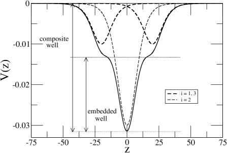
Figure 1: A sum of 3 MPT potentials yields an embedded quantum well in another well. Here $V(z)$ is in units of $\hbar^{2}/m^{*}$ and $z$ is in angstrom.

2 The Quantum Well-in-a-Well Model

A quantum well-in-a-well can be constructed from a sum of three MPT potentials, that is,

$$V(z)=-\left(\frac{\hbar^{2}\alpha^{2}}{2m^{*}}\right)\sum_{i=1}^{3}\frac{\lambda_{i}(\lambda_{i}-1)}{\cosh^{2}[\alpha(z+d_{i})]}\;,$$ (1)

where $m^{*}$ is the effective mass and $\hbar$ is Dirac’s constant. The well-in-a-well system consists of two left and right wells, labelled with indices $i=1$ and $i=3$, respectively, and a center well denoted by index $i=2$. Their location relative to the origin are $d_{1}=-d$, $d_{2}=0$, and $d_{3}=+d$. In this work, the width parameter $\alpha$ is the same for all wells studied and it is kept to a constant value of $0.1\;\AA^{-1}$. Only the value of the depth parameter $\lambda$ is varied. Here the depth parameters of the side wells, $i_{1}\;\;\&\;\;i_{3}$, are set equal, that is, $\lambda_{1}=\lambda_{3}$. This is done to retain the symmetric shape of the well about the origin. The middle well has a depth parameter $\lambda_{2}$ and its value can be different from $\lambda_{1}$. By varying the values of $\lambda_{1}$, $\lambda_{2}$ and the shift parameter $d$, the size of the effective embedded potential well relative to the resulting main quantum well can be controlled. Figure 1 illustrates a composite well as obtained from its constituent potential wells. Note that the model represents the conduction band of a quantum well system.

3 The Numerical Method

The bound states of a single electron in the composite well system described above can be obtained by using Eq. (1) in the Schrödinger equation in one dimension

$$\left[-\frac{\hbar^{2}}{2m^{*}}\frac{\partial^{2}}{\partial z^{2}}+V(z)\right]\psi(z)=E\psi(z)\;.$$ (2)

It follows that the wavefunction can be determined through an iterative procedure from Eq. (2) in the central difference form Harrison00 , that is,

$$\psi(z+\delta z)=\frac{2m^{*}}{\hbar^{2}}(\delta z)^{2}[V(z)-E]\psi(z)$$

$$+2\psi(z)-\psi(z-\delta z)\;.$$ (3)

Here $\delta z$ is an arbitrary infinitesimal step size and the initial values of $\psi(z)$ and $\psi(z-\delta z)$ are obtained via simple symmetry arguments. The advantage of using the MPT potentials is that the eigenenergies of a single MPT potential is known analytically Flugge74 . Hence, the difference in energy states of the constructed composite well as compared to the single MPT well can be related to the potential parameters.

The shooting method Harrison00 is implemented in this work to obtain each energy eigenvalue in a given energy range. Each solution must satisfy the boundary conditions that $\psi(z)$ and its derivative vanish at infinity. In addition to the boundary conditions, the minimum tolerance set for numerical convergence of $\psi$ and its derivative is $10^{-10}$. To accurately obtain the bound states, the whole potential depth is scanned to check for energy intervals wherein the first derivative of the wavefunction changes sign at infinity. This signals that within this energy range a bound state can be found. The bisection method is then applied to this particular interval to search for the bound state with a convergence limit of $\Delta E=10^{-10}\hbar^{2}/m^{*}$.

Another property of this well-in-a-well system that will be studied here is the scattering of a free particle from this potential landscape via the transfer matrix approach. The transmission probability is obtained from the ratio between the amplitude of the transmitted wave ($A_{T}$) and that of the incident wave ($A_{I}$)

$$|T|^{2}=\left(\frac{|A_{T}|}{|A_{I}|}\right)^{2}=\frac{1}{|M_{11}|^{2}}\;.$$ (4)

The transfer matrix technique yields Rodriguez06 ; Singh97

$$M_{11}=\frac{1}{2}\left[1+\frac{\kappa(z+\delta z)}{\kappa(z)}\right]e^{i[\kappa(z+\delta z)-\kappa(z)]z}\;,$$ (5)

where $\kappa(z)=\left(2m^{*}[E-V(z)]\right)^{1/2}/\hbar$. Here $E$ is the incident particle’s kinetic energy. It is further assumed here that the effective mass does not vary in space. Length measurements are given in angstroms and energy measurements are in units of ${\hbar^{2}}/{m^{*}}$.

4 Results and Discussion

Figure 2 shows a quantum well-in-a-well system, whose subwell size is 24$\%$ of the full well depth. The properties of the composite well is studied using a single MPT well of the same depth as a benchmark. In addition, a parabolic well having the same width is fitted to the composite well for comparison. The same approach is used to obtain the bound states for the single MPT well and the parabolic well.

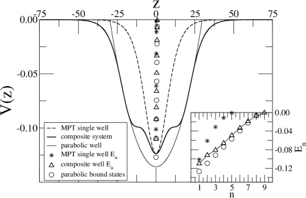
Figure 2: Bound states of a composite quantum well-in-a-well system as compared to a single MPT well of the same depth and a parabolic well of the same width. For the composite system, the constituent well parameters are $\lambda_{1}=\lambda_{3}=4.5$, $\lambda_{2}=5.0$ and $d=16\;\AA$, while for the single MPT well $\lambda=5.4992$. The inset shows the eigenenergies $E_{n}$ where $n$ is the bound state index.

One finds that the composite well’s ground state is lower by $\approx 9\%$ relative to the ground state of the single MPT well of the same depth. In this example, the ground state of the parabolic well is lowest as expected due to its deeper potential depth. Note that the composite well has more bound states than that of single MPT well of the same depth or the parabolic well of the same width. Further, the interval between bound states are more evenly distributed in the composite system as compared to the single MPT well. The distribution of states for the composite well is more similar to the even distribution of energy states of a parabolic well of the same width rather than that of the single MPT potential.

Next, Fig. 3 illustrates three well-in-a-well systems of the same depth, symmetry and base width. The latter is the potential width at $V(z)=0$. What varies in this plot is the depth of the component side wells yielding systems having different depths of embedded wells. Figure 3 shows systems with embedded wells of depths (A) 88$\%$, (B) 64$\%$ and (C) 28$\%$ relative to the composite well’s full depth.

The corresponding bound states of the three composite wells are shown in Fig. 4. As the depth of the component side wells increases the number of bound states also increases. Thereby, well (C) has the most number of bound states. Furthermore, the change in slope of the plot of eigenstate $E_{n}$ relative to the bound state index $n$, towards a constant value indicates the shift towards an even distribution of the energy states. This occurs for the case of well (C) since the shape of the edge of this well approaches that of a parabolic potential. Recall that for the case of the simple harmonic potential well, the energy levels are evenly distributed. So as the bottom of the component side wells approaches the depth of the middle well, we expect a straight line. However, near the base of the potential the shape retains the tail of a modified Pöschl-Teller potential well, hence the last two bound states are nearer to each other as compared to those adjacent states in the middle and edge of the well.

Figure 3: Three quantum well-in-a-well systems having equal depth and base width. The other potential parameters are (A.) $d=27\;\AA$, $\lambda_{1}=\lambda_{3}=2$ and $\lambda_{2}=5$, (B.) $d=21\;\AA$, $\lambda_{1}=\lambda_{3}=3.00$ and $\lambda_{2}=4.92$, and (C.) $d=16\;\AA$, $\lambda_{1}=\lambda_{3}=4.00$ and $\lambda_{2}=4.59$.

Figure 4: The bound states of the three well systems shown in Fig. 3.

Another phenomenon which is affected by the potential is the transport of a particle above it. Recall that in the case of a finite rectangular well of width $L$, or similarly, a potential barrier of the same width, transmission resonance is observed when the wave number takes on integral multiples of $\pi/L$ Harrison00 . It has also been demonstrated that a low energy incident electron above a rectangular well may be captured into a bound state due to dissipation CaiHZY90 . Transmission resonance is only restored for particle kinetic energies beyond the ”captive” energy region CaiHZY90 .

In the case of scattering above a single MPT potential, transmission resonance is observed when $\lambda$ is an integer regardless of the magnitude of the kinetic energy of the incident particle Flugge74 . Unlike in the well-in-a-well systems studied here, there are no resonant wells. This is true even for well (A) in which its constituent wells, by themselves, are absolute transparent potentials. Figure 5 shows the transmission probability of a free particle with effective mass $m^{*}$ above each composite well in Fig. 3. A particle has a lower probability of transmission if the kinetic energy of the particle approaches zero. As expected, the larger the kinetic energy of the incident particle the more likely it is to be transmitted. The monotonic increasing trend of the transmission probability for the composite wells remains valid even when the well width is increased. This is in contrast to the appearance of an oscillatory nature of the transmission coefficient when the width of a finite rectangular well is widened.

The behavior of interest is that well (A) has the lowest probability of transmission relative to systems (B) and (C). Note that for a particle scattered in a finite rectangular well in the non-resonance regime, the transmission probability increases with decreasing depth and width. The opposite behavior is, thus, observed here, wherein the most shallow side wells and the most narrow middle well yield a composite system that creates more disturbance to particle transmission. In the perspective of an incident particle with energies corresponding to $0.2(m^{*})^{1/2}/\hbar<k<0.6(m^{*})^{1/2}/\hbar$, wells (B) and (C) are more slowly varying potential functions relative to well (A). The abruptness of the change in the potential in (A) provides a stronger force in reducing the probability of transmission in this $k$ regime.

Figure 5: The corresponding transmission probability of an incident free particle, with energy $E>0$, scattered on each well as shown in Fig. 3. Here $k$ is the magnitude of the free particle’s wave vector and is given in units of $(m^{*})^{1/2}/\hbar$.

5 Summary

This paper presented a simulation model for a composite quantum well-in-a-well system and investigated the quantum mechanical properties arising from such construction. A superposition of modified Pöschl-Teller potentials is chosen for the model because the constituent wells can easily be varied without increasing the numerical complexity in solving the Schrödinger equation. This work showed that deviations in quantum well structures of the same functional form and depth yield entirely different properties as shown in the differences in their ground state energies, the number and distribution of bound states and the transmission probabilities of an incident free particle above the composite wells. Tailor-made quantum well systems as presented here offer ease and flexibility that can be suited to desired features for application purposes.

References

- [1] L. Brey, N.F. Johnson, and B.I. Halperin. Phys. Rev. B 40 (1989) 10647.
- [2] A. Laakso, M. Dumitrescu, L. Toikkanen, A. Tukiainen, and V. Rimpiläinen and M. Pessa. Optical and Quantum Electronics (2007), doi:10.1007/s11082-007-9155-8.
- [3] K.A. Kaduki, A. Ghiti, W. Batty, and D.W.E. Allsopp. Phys. Scripta 67 (2003) 68.
- [4] S. Tomić, V. Milanović, and Z. Ikonić. Phys. Rev. B 62 (2000) 16681.
- [5] J. Radovanović, V. Milanović, Z. Ikonić, and D. Indjin. Phys. Rev. B 59 (1999) 5637.
- [6] S. Flügge. Practical Quantum Mechanics. Springer-Verlag, Berlin, 1974.
- [7] H. Kleinert and I. Mustapic. J. Math. Phys. 33 (1992) 643.
- [8] N. Rosen and P.M. Morse. Phys. Rev. 42 (1932) 210.
- [9] A. Rodriguez. J. Phys. A: Math. Gen. 39 (2006) 14303.
- [10] P. Harrison. Quantum Wells, Wires and Dots: Theoretical and Computational Physics. John Wiley & Sons, Chichester, 2000.
- [11] J. Singh. Quantum Mechanics: Fundamentals and Applications to Technology. John Wiley, New York, 1997.
- [12] W. Cai, P. Hu, T.F. Zheng, B. Yudanin and M. Lax. Phys. Rev. B 41 (1990) 3513.