Dynamics of a stretched nonlinear polymer chain

Abstract

We study the relaxation dynamics of a coarse-grained polymer chain at different degrees of stretching by both analytical means and numerical simulations. The macromolecule is modelled as a string of beads, connected by anharmonic springs, subject to a tensile force applied at the end monomer of the chain while the other end is fixed at the origin of coordinates. The impact of bond non-linearity on the relaxation dynamics of the polymer at different degrees of stretching is treated analytically within the Gaussian self-consistent approach (GSC) and then compared to simulation results derived from two different methods: Monte-Carlo (MC) and Molecular Dynamics (MD).

At low and medium degrees of chain elongation we find good agreement between GSC predictions and the Monte-Carlo simulations. However, for strongly stretched chains the MD method, which takes into account inertial effects, reveals two important aspects of the nonlinear interaction between monomers: (i) a coupling and energy transfer between the damped, oscillatory normal modes of the chain, and (ii) the appearance of non-vanishing contributions of a continuum of frequencies around the characteristic modes in the power spectrum of the normal mode correlation functions.

I Introduction

The dynamics of a linear polymer was first studied and solved by Rouse in his seminal paper Rouse on the relaxation behavior of a phantom (ideal) chain of volumeless beads connected by harmonic (linear) springs. This model, which reveals the transcendental features of a linear chain, gives all characteristic dynamic values for nearly free chains whereby the assumed linearity of the model provides a good description of the process under investigation. Since this simplified model fails to retain the physics when the chain is subjected to strong tensile forces (large stretching), several approaches have been suggested which take into account the finite extensibility of the chain. Most of them are based on modifying the underlying force between monomers, whose nonlinear nature manifests itself for high extensions. Among the earlier studies that have been tried to understand the dynamics of highly stretched polymers one should mention the work of Pincus Pincus77 which considered internal modes of a strongly stretched chain using the blob model DeGennes79 . Based on this work, Marciano and Brochart-Wyart Marciano95 , studied a single chain stretched by a force $f$ applied at the free end and fixed with the other end at the origin. They demonstrated that stretched chains can be thought as Rouse chains of impenetrable blobs where all the blobs are identical. In the long wave-length limit chain dynamics is described by renormalized Rouse modes of mode number $p$ with a dispersion relation for the corresponding relaxation times $\tau_{p}\propto p^{-2}$. More recently, the work of Hatfield and Quake Hatfield99 presented theoretical calculations and computer simulations to estimate the effects of tension and hydrodynamics on $\tau$, the fundamental relaxation time of the polymer.

Apparently none of these studies, however, seems to have reached a complete and definite description of the problem, in spite of its fundamental nature. In view of many experiments and technological applications, the dynamics of highly stretched chains results fundamental in studying bond rupture of filled and unfilled elastomers. So far, there no theory based on molecular models for the fracture of materials exists. Most of the existing theories are based on phenomenological ideas, which consider directly the material parameters Busfield99 ; Gurtin00 ; Gross01 ; Gross02 ; Haupt95 ; Persson08 ; Hamed94 . In this work, the main emphasis is drawn on developing molecular pictures for breaking chains, unfilled and filled elastomers. It turns out quickly that the basic problems concerning the behavior of strongly stretched chains are not treated in such a way, that a systematic study on the chain breaking mechanism can be carried out. Therefore we concentrated ourselves basically to study the dynamics of highly stretched chains. To do so, there are two different ways to tackle this problem. The most obvious possibility is to introduce constraints, where the lengths of the chain segments are fixed at any times during the dynamical processes. Such a theory requires the introduction of Lagrange multipliers. The theory can be formulated on an exact way, but nevertheless the solution needs many approximations, which are not always easy to control. The corresponding stochastic equations are highly non-linear and do not allow the complete determination of the Langrange multipliers Doi .

To be more specific, we state the problem which we are going to discuss below in some more details. Polymer dynamics is usually studied by the so-called Rouse equation, which has its origin in the corresponding Edwards Hamiltonian for Gaussian Chains. In discrete notation Gaussian chains are described by a Gaussian chain statistics, which is defined by the Hamiltonian

$$H=k_{B}T\frac{3}{2b_{0}^{2}}\sum_{i=1}^{N}{\bf b}_{i}^{2}$$ (1)

where $k_{B}T$ is the thermal energy, ${\bf b}_{i}={\bf r}_{i}-{\bf r}_{i-1}$ the individual bond vectors of a chain defined by a connected set of position vectors $\{{\bf r}_{i}\}$ and $b_{0}^{2}$ their mean value. The Rouse equation, which is the Langevin equation for the monomer position vector ${\bf r}_{i}$ is simply defined by the equation of motion

$$\xi_{0}\frac{\partial{\bf R}(s,t)}{\partial t}-\frac{3k_{B}T}{b_{0}^{2}}\frac{\partial^{2}{\bf R}(s,t)}{\partial s^{2}}={\bf h}(s,t)$$ (2)

where ${\bf r}_{i}$ has been represented by continuous space curves $\textbf{R}(s,t)$ and $s$ is the arc length variable running from 0 to $L$ along chain contour. In last equation, the first term corresponds to the frictional force, $\xi_{0}$ being the friction coefficient and $\textbf{h}(s,t)$ is the stochastic force, which is taken as a white noise. The second term is nothing but the elastic force, and is easily derived by the gradient of the Hamiltonian $H$. The drawback of this simple stochastic equation is, that the bond vectors can be stretched to infinity and thus Gaussian chains overstretch.

This drawback is normally repaired by the use of rigid constraints, which fix the bond length strictly to $|{\bf b}_{i}|=|{\bf r}_{i}-{\bf r}_{i-1}|=b_{0}$, but this yields to all the problems discussed above. The alternative possibility is the use of potentials, which do not allow the chain to extend to infinity at high external forces instead of hard constraints. Although this corresponds to a very different approach the problems become to some extend more feasible. As an example we mention the FENE - potential Kremer , which is widely used in computer simulations, to prevent the overstretching of the chains and avoiding so unphysical conformations. To do so we have proposed a modified chain potential according to the FENE - potential, where the chain segments can only stretch to a maximum value, i.e.,

$$\beta H=-\frac{3}{2}\sum_{i=1}^{N}\ln\left(1-\frac{b_{i}^{2}}{b_{0}^{2}}\right)$$ (3)

where we have chosen here just for the maximum extension of the bonds the mean bond size from above (in this eq. this is done for illustration, for the more specific calculations and simulations we have chosen more general cases). The distribution function for the end-to-end vector contains Bessel functions that makes it not very suitable for analytical computations. Nevertheless in a crude approximation it can be shown, that its asymptotics is of the form

$$G({\bf R},N)\propto\exp\left(\frac{3R^{2}}{2Nb_{0}^{2}}\frac{1}{(1-(R/(Nb_{0}))^{2})^{1/2}}\right)$$ (4)

which shows that the end vector distribution function $G({\bf R},N)$ tends to zero when the chain is close to its maximum extension $R=Nb_{0}$.

Concerning the dynamics we can also extract some features of the FENE - type potential. For small elongations, $|{\bf b}_{i}|<<b_{0}$ the FENE - Hamiltonian yields back the Gaussian chain and so, in the dynamics the classical Rouse equation. On the other hand it provides the basis for a non-linear dynamical polymer model, which can be summarized in the (approximate) non-linear stochastic equation,

$$\xi_{0}\frac{\partial{\bf R}(s,t)}{\partial t}-\frac{3k_{B}T}{b_{0}^{2}}\dfrac{\frac{\partial^{2}{\bf R}(s,t)}{\partial s^{2}}}{1-\frac{1}{b_{0}^{2}}\left(\frac{\partial{\bf R}(s,t)}{\partial s}\right)^{2}}={\bf h}(s,t)$$ (5)

Our intention in the present work is to examine the fundamental aspect of bond nonlinearity of the chain in the high stretched limit and its impact on the polymer relaxation dynamics with analytical methods and simulation techniques. To this end we first employ the Gaussian self-consistent approach. The method has been extensively used (see e.g. Timo ) and appears to provide an adequate approach to study this type of problems. In addition, we run Monte-Carlo (MC) simulations to compute and compare the dynamical behavior with that, predicted by the analytical approach. It is worth noting that the MC scheme does not take into account mass in the model. In this sense, we want to know to what extent this is a good description of the problem. To answer this question, we also performed Molecular Dynamics (MD) simulations since at high degrees of chain extension the effects of mass and inertia may not be neglected; therefore we have to modify the equation of motion as follows:

$$m_{b}\frac{\partial^{2}{\bf R}(s,t)}{\partial t^{2}}+\xi_{0}\frac{\partial{\bf R}(s,t)}{\partial t}-\frac{3k_{B}T}{b_{0}^{2}}\dfrac{\frac{\partial^{2}{\bf R}(s,t)}{\partial s^{2}}}{1-\frac{1}{b_{0}^{2}}\left(\frac{\partial{\bf R}(s,t)}{\partial s}\right)^{2}}={\bf h}(s,t)$$ (6)

The extension by the inertia term is to first instance not obvious, though it is intuitive. The dynamics of strongly stretched chains will always get vibrational modes, whenever non-linear springs are connecting the beads. In contrast to the Gaussian chains, which can be stretched to infinity, the springs take at large stretching forces more and more energy, which will manifest itself in travelling waves along the longitudinal direction of the stretched string. Of course this FENE Rouse model is also only an approximation, since rigid constraints cannot be described rigorously by any (soft) potential. Nevertheless it removes the basic non-physical features from the Gaussian chain model. The chain possesses a finite extensibility and the distribution function does not contain unphysical (overstretched) states.

Form this equation we can expect several new features compared to the Rouse equation.

1. We can expect diverging time scales as long as the chain becomes strongly extended, i.e., close to the maximum deformation, where only chain fluctuations close to the maximum stretching of the individual bonds matter. These diverging time scales will be imposed by the singularity in the stretching force term.

2. We can expect a “transition” from relaxational dynamics to a travelling wave dynamics. At low deformation states the dynamics is mainly ruled by fluctuations where the FENE nature does not play a crucial role. Thus at low deformations we readily expect a Rouse type dynamics. At larger stretching ratios, we have basically a linear chain (like in one dimensional mono atomic solids) and “acoustic phonon modes” can be expected, if the springs were harmonic.

3. Since the springs are highly anharmonic we can expect non-trivial features for the chain dynamics. At high stretching ratios, i.e., at large stretching forces, we might have strong effects from the non-linearity of the potential. At small deformations the Rouse equation is still a valid and useful approximation, at large deformations, however, the “Rouse modes” will interact with each other, they will exchange energy and damped solitary wave excitations will appear.

However for the main conclusions the form and power of the singularity in the modified force term in eq.(6) is not very important. The main issue is that a singularity at full extension of the bonds, i.e, the chain appears. Another aspect is that we have so far ignored the orientation of the chain upon stretching, which will simplify the problem slightly since we will split the isotropic variable $\bf{R}(s)$ into its direction perpendicular and parallel to the force. It is then physically obvious that both components will respond differently to the strong stretching force.

In the following we will discuss these ideas in more details. In the first step we will show how simple linearizations will provide first ideas to the general problem. There we see how the nonlinearity changes the character of the dynamics completely, when the chains are strongly elongated. The simple analytic model will also provide the differences in the behavior of the two components $R_{\perp}(s)$ and $R_{||}(s)$. In the second part of the paper we will use simulations to go beyond the linear analytical approach. We shall see that the simulation results provide important new information on the chain dynamics in the high stretching regime.

II Gaussian self-consistent approach

To proceed in a first step with the analytical theory we have chosen to employ a self consistent Gaussian approach, i.e., a variational technique, which allows to get a first feeling for the behavior of such strongly elongated chains. The first step is, that for such stretched chains with finite extensibility we cannot argue anymore in looking at the isotropic chain variables themselves. Therefore the chain vectors need to be separated into components parallel and perpendicular to the stretching direction. Despite the mean field, and the linearization character, this will provide some important insight to the physics of the problem.

The dynamics of a stretched polymer chain at high degree of stretching is essentially nonlinear. This is due to the necessity of large forces being applied over a short region of space so as to prevent the chain from stretching indefinitely. While in the Rouse (linear) model, the linear springs that provide the connectivity of the chain fail to meet this condition, it is well satisfied by the anharmonic springs, described by the frequently used finite extensible nonlinear elastic (FENE) potential. However, we treat first the relaxation dynamics of a stretched polymer chain by solving the nonlinear Langevin equation within the framework of the Gaussian self-consistent approach (GSC). To do so we considered a polymer chain with $N$ monomers connected by FENE springs, with one chain end fixed at the origin of coordinates and pulled by force $f$ at the opposite chain end. Due to the external force $f$, there emerges a preferred direction in space leading to symmetry breaking in the problem, caused by extending the polymer in direction of the acting force. This effect splits the dynamics of the chain into two directions Hatfield99 with respect to monomers motion, ${\bf R}(s,t)$, one parallel to the force and the other perpendicular to it, leading to distinct longitudinal and transverse relaxation times. For the equation of motion of the statistically averaged position, $\bar{R}_{\parallel}(s,t)\equiv\langle R_{\parallel}(s,t)\rangle$, in direction parallel to force, we have

$$\xi_{0}\frac{\partial\bar{R}_{\parallel}(s,t)}{\partial t}+\left\langle\frac{\delta V[{\bf R}(s,t)-{\bf R}(s-1,t)]}{\delta R_{\parallel}(s,t)}\right\rangle+\left\langle\frac{\delta V[{\bf R}(s,t)-{\bf R}(s+1,t)]}{\delta R_{\parallel}(s,t)}\right\rangle-f\delta_{sN}=0$$ (7)

where $V[{\bf R}(s,t)-{\bf R}(s\pm 1,t)]$ refers to the non-linear potential (FENE in this case) which links the nearest neighbors along the chain backbone and $\xi_{0}$ denotes the friction coefficient of a single monomer. We introduce the notation, $\bar{R}_{\parallel}(s,t)=\langle R_{z}(s,t)\rangle$. In direction perpendicular to force, the first moments are $\bar{R}_{x}(s,t)=\bar{R}_{y}(s,t)\equiv\bar{R}_{\perp}(s,t)=0$ due to axial symmetry. Additionally, we present the equations of motion for time displaced correlation functions; in the perpendicular direction $C_{\perp}(s,n,t,t^{\prime})\equiv\langle R_{\perp}(s,t)R_{\perp}(n,t^{\prime})\rangle$ we write

$$\xi_{0}\frac{\partial C_{\perp}(s,n,t,t^{\prime})}{\partial t}+\left\langle R_{\perp}(n,t^{\prime})\frac{\delta V[{\bf R}(s,t)-{\bf R}(s-1,t)]+V[{\bf R}(s,t)-{\bf R}(s+1,t)]}{\delta R_{\perp}(s,t)}\right\rangle=\\ \langle R_{\perp}(n,t^{\prime})h_{\perp}(s,t)\rangle$$ (8)

and for the parallel counterpart $C_{\parallel}(s,n,t,t^{\prime})\equiv\langle R_{\parallel}(s,t)R_{\parallel}(n,t^{\prime})\rangle$

$$\xi_{0}\frac{\partial C_{\parallel}(s,n,t,t^{\prime})}{\partial t}+\left\langle R_{\parallel}(n,t^{\prime})\frac{\delta V[{\bf R}(s,t)-{\bf R}(s-1,t)]+V[{\bf R}(s,t)-{\bf R}(s+1,t)]}{\delta R_{\parallel}(s,t)}\right>-f\bar{R}_{\parallel}(n,t^{\prime})\delta_{sN}=\\ \langle R_{\parallel}(n,t^{\prime})h_{\parallel}(s,t)\rangle$$ (9)

where $h_{\parallel}(s,t)$ and $h_{\perp}(s,t)$ are random Gaussian $\delta$-correlated forces in parallel and perpendicular directions respectively. We also study the equal time correlation functions $C_{\parallel,\perp}(s,n,t,t)=C_{\parallel,\perp}(s,n,t)$ which in the steady state regime do not depend on the time $t$. For the perpendicular direction, we have

$$\xi_{0}\frac{\partial C_{\perp}(s,n,t)}{\partial t}+K_{\perp}(s,s-1)[C_{\perp}(n,s,t)-C_{\perp}(n,s-1,t)]+K_{\perp}(s,s+1)[C_{\perp}(n,s,t)-C_{\perp}(n,s+1,t)]$$

$$+K_{\perp}(n,n-1)[C_{\perp}(s,n,t)-C_{\perp}(s,n-1,t)]+K_{\perp}(n,n+1)[C_{\perp}(s,n,t)-C_{\perp}(s,n+1,t)]=2\delta_{ns}k_{B}T$$ (10)

and for the parallel,

$$\xi_{0}\frac{\partial A_{\parallel}(s,n,t)}{\partial t}+K_{\parallel}(s,s-1)[A_{\parallel}(n,s,t)-A_{\parallel}(n,s-1,t)]+K_{\parallel}(s,s+1)[A_{\parallel}(n,s,t)-A_{\parallel}(n,s+1,t)]$$

$$+K_{\parallel}(n,n-1)[A_{\parallel}(s,n,t)-A_{\parallel}(s,n-1,t)]+K_{\parallel}(n,n+1)[A_{\parallel}(s,n,t)-A_{\parallel}(s,n+1,t)]=2\delta_{ns}k_{B}T$$ (11)

Here, we define $A_{\parallel}(s,n,t)=C_{\parallel}(s,n,t)-\bar{R}_{\parallel}(s,t)\bar{R}_{\parallel}(n,t)$, and the effective nearest neighbor constant, $K_{\parallel,\perp}(s,s\pm 1)$, is defined by eq. (40) in the Appendix. The relationship $\langle 2R_{\perp}(n,t)h_{\perp}(s,t)\rangle=2\delta_{ns}k_{B}T$ is also derived explicitly in Appendix A.

II.1 First cumulant expansion

Consider first the term $\left\langle\frac{\delta V[{\bf R}(s,t)-{\bf R}(s-1,t)]}{\delta R_{\parallel}(s,t)}\right\rangle$ which is the average force experienced by each monomer. The calculation yields

$$\left\langle\frac{\delta V[{\bf R}(s,t)-{\bf R}(s-1,t)]}{\delta R_{\parallel}(s,t)}\right\rangle=\left\langle\frac{\delta}{\delta R_{\parallel}(s,t)}\int d^{3}r\delta[{\bf R}(s,t)-{\bf R}(s-1,t)-r]V(\vec{r})\right\rangle=$$

$$=-\int d^{3}r\left\langle\frac{\partial}{\partial r_{\parallel}}\delta[{\bf R}(s,t)-{\bf R}(s-1,t)-r]\right\rangle V(\vec{r})=\int d^{3}r\langle\delta[{\bf R}(s,t)-{\bf R}(s-1,t)-r]\rangle\frac{\partial V(\vec{r})}{\partial r_{\parallel}}$$

The key point is then to determine the difference $\langle\delta[{\bf R}(s,t)-{\bf R}(s-1,t)-r]\rangle$. This is accomplished by employing the following crucial approximation $\langle\delta[{\bf R}(s,t)-{\bf R}(s-1,t)-r]\rangle\approx\delta[\langle{\bf R}(s,t)-{\bf R}(s-1,t)-r\rangle]$ which comes from retaining only the first term in the cumulant expansion. Taking into account that $V(\vec{r})=-\frac{1}{2}k_{F}b_{0}^{2}\ln(1-\frac{\vec{r}^{2}}{b_{0}^{2}})$ and $\vec{r}^{2}=r_{\parallel}^{2}+r_{\perp}^{2}$ one arrives at

$$\int d^{3}r\langle\delta[{\bf R}(s,t)-{\bf R}(s-1,t)-r]\rangle\frac{\partial V(\vec{r})}{\partial r_{\parallel}}\approx k_{F}\frac{\bar{R}_{\parallel}(s,t)-\bar{R}_{\parallel}(s-1,t)}{1-\left[\frac{\bar{R}_{\parallel}(s,t)-\bar{R}_{\parallel}(s-1,t)}{b_{0}}\right]^{2}}$$

II.2 Steady state solution

In order to obtain the steady state solution of eq.(7), we set $\frac{\partial\bar{R}_{\parallel}(s,t)}{\partial t}=0$. Then, we can find $\bar{R}_{\parallel}(1)$ by adding up the $N$ terms for the $\bar{R}_{\parallel}(s)$, requiring that the boundary conditions of the problem are $\bar{R}_{\parallel}(0)=0$ (first monomer is fixed at the origin of coordinates), and $\bar{R}_{\parallel}(N+1)-\bar{R}_{\parallel}(N)=0$ (free end condition).

Eventually we get

$$f=k_{F}\frac{\bar{R}_{\parallel}(1)}{1-\left(\frac{\bar{R}_{\parallel}(1)}{b_{0}}\right)^{2}}$$ (12)

from which one can easily derive $\bar{R}_{\parallel}(1)=\frac{k_{F}b_{0}^{2}}{2f}\left(-1+\sqrt{1+\frac{4f^{2}}{k_{F}^{2}b_{0}^{2}}}\right)$. In Figure (1) we plot the elongation $\bar{R}_{\parallel}(1)$ as a function of $f$.

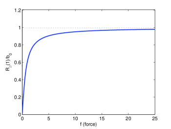
Figure 1: Variation of the bond length between adjacent beads in a chain with applied tensile force $f$. Eventually, for large forces the bond length approaches asymptotically its maximum value $b_{0}$.

Applying an iteration procedure, a general expression for $\bar{R}_{\parallel}(s)$ can be found, $\bar{R}_{\parallel}(s)=s\bar{R}_{\parallel}(1),\ 1<s\leq N$. Setting $\frac{\partial C_{\parallel,\perp}(s,n,t)}{\partial t}=0$, the steady state solution for the equal time correlators can also be obtained. Then, for the perpendicular direction, the final equation reads

$$K_{\perp}(s,s-1)[C_{\perp}(n,s)-C_{\perp}(n,s-1)]+K_{\perp}(s,s+1)[C_{\perp}(n,s)-C_{\perp}(n,s+1)]$$

$$+K_{\perp}(n,n-1)[C_{\perp}(s,n)-C_{\perp}(s,n-1)]+K_{\perp}(n,n+1)[C_{\perp}(s,n)-C_{\perp}(s,n+1)]=2\delta_{ns}k_{B}T,$$ (13)

and for the parallel

$$K_{\parallel}(s,s-1)[A_{\parallel}(n,s)-A_{\parallel}(n,s-1)]+K_{\parallel}(s,s+1)[A_{\parallel}(n,s,t)-A_{\parallel}(n,s+1)]$$

$$+K_{\parallel}(n,n-1)[A_{\parallel}(s,n)-A_{\parallel}(s,n-1)]+K_{\parallel}(n,n+1)[A_{\parallel}(s,n)-A_{\parallel}(s,n+1)]=2\delta_{ns}k_{B}T$$ (14)

The solution for the time-independent correlator $C_{\perp}(s,n)$ is found by rearranging eq. (II.2) which makes it possible to take its continuum limit and rewrite it in a more convenient way. Eventually, we get

$$K_{\perp}\left(\frac{\partial^{2}C_{\perp}(n,s)}{\partial s^{2}}+\frac{\partial^{2}C_{\perp}(n,s)}{\partial n^{2}}\right)=-2\delta(n-s)k_{B}T$$ (15)

where $K_{\perp}(s,s\pm 1)=K_{\perp}(n,n\pm 1)\equiv K_{\perp}=\frac{k_{F}}{1-\left(\frac{\bar{R}_{\parallel}(1)}{b_{0}}\right)^{2}}$. It is better here to define this constant by the relative degree of stretching $\lambda=\frac{N\bar{R}_{\parallel}(1)}{\sqrt{N}b_{0}}$ and its maximum value, $\lambda_{max}=\frac{Nb_{0}}{\sqrt{N}b_{0}}=\sqrt{N}$ (where $Nb_{0}$ denotes the total contour length of the chain). Thus one can rewrite $K_{\perp}=\frac{k_{F}}{1-\left(\frac{\lambda}{\lambda_{max}}\right)^{2}}$.

Equation (15) is a linear equation which can be easily solved for example by means of the Green’s function method Morse . In the same way, one can rearrange equation (II.2) and proceed in a similar fashion. The final solutions reads

$$C_{\parallel,\perp}(n,s)=\sum_{p=1}\frac{4}{N}\frac{k_{B}T}{K_{\parallel,\perp}}\frac{2N^{2}}{(2p-1)^{2}\pi^{2}}\sin\left(\frac{(2p-1)\pi n}{2N}\right)\sin\left(\frac{(2p-1)\pi s}{2N}\right)$$ (16)

where $K_{\parallel}(s,s\pm 1)=K_{\parallel}(n,n\pm 1)\equiv K_{\parallel}=k_{F}\frac{1+\left(\frac{\lambda}{\lambda_{max}}\right)^{2}}{\left[1-\left(\frac{\lambda}{\lambda_{max}}\right)^{2}\right]^{2}}$. These two coupling (effective spring) constants behave therefore differently in the two directions and depend in a detailed way on the deformation ratio. Both spring constants show a singularity at the maximum deformation. We will use these results again in the last section of these paper, when we discuss the limiting cases and the physics of the numerical results, which will follow later.

II.3 Time displaced correlators

The steady state solution for $C_{\parallel,\perp}(n,s)$ offers an initial condition from which the time dependent problem can be solved. Following the GSC method, we are now in a position to solve the equations of motion also for $C_{\perp}(s,n,t,t^{\prime})$. Using the causality conditions of physical systems $\langle R_{\perp}(n,t^{\prime})h_{\perp}(s,t)\rangle=0$ for $t^{\prime}<t$, and the same calculations outlined in the previous section, after taking the continuum limit, one finally arrives at

$$\xi_{0}\frac{\partial C_{\perp}(n,s,t,t^{\prime})}{\partial t}=K_{\perp}\left(\frac{\partial^{2}C_{\perp}(n,s,t,t^{\prime})}{\partial s^{2}}\right).$$ (17)

This is one-dimensional diffusion equation that can easily be solved to give

$$C_{\perp}(n,s,t,0)=\sum_{p=1}A_{p}\exp\left(-\beta_{p}\frac{K_{\perp}}{\xi_{0}}t\right)\sin\left(\frac{(2p-1)\pi s}{2N}\right)$$ (18)

where $\beta_{p}=\frac{(2p-1)^{2}\pi^{2}}{4N^{2}}$ and we have chosen $t^{\prime}=0$ without loss of generality. The amplitudes $A_{p}$ may be determined from the initial condition since $C_{\perp}(n,s,0,0)=C_{\perp}(n,s)$. Equating the expression for $C_{\perp}(n,s,t,0)$ at $t=0$, (eq. 18), and $C_{\perp}(n,s)$, one arrives at

$$A_{p}=\frac{4}{N}\frac{k_{B}T}{K_{\perp}}\frac{2N^{2}}{(2p-1)^{2}\pi^{2}}\sin\frac{(2p-1)\pi n}{2N}.$$ (19)

Evidently, $A_{p}$ is a function of $(p,n)$ since $C_{\perp}(n,s,t,0)$ is a function of $(n,s,t)$. Now, it is possible to write down the final expression for $C_{\perp}(n,s,t,0)$ as

$$C_{\perp}(n,s,t,0)=\sum_{p=1}\sum_{m=1}\frac{4}{N}\frac{k_{B}T}{K_{\perp}}\frac{\delta_{pm}}{\frac{(2p-1)^{2}\pi^{2}}{2N^{2}}+\frac{(2m-1)^{2}\pi^{2}}{2N^{2}}}e^{-\beta_{p}\frac{K_{\perp}}{\xi_{0}}t}\sin\left(\frac{(2p-1)\pi n}{2N}\right)\sin\left(\frac{(2m-1)\pi s}{2N}\right)$$ (20)

Following the same reasoning one can obtain an identical solution for the parallel direction too by replacing $K_{\perp}\rightarrow K_{\parallel}$. From the last equation, the (Rouse) mode amplitudes can be calculated in a straightforward manner:

$$\langle X_{p\perp,\parallel}(t)X_{m\perp,\parallel}(0)\rangle=\frac{k_{B}T}{K_{\perp,\parallel}}\delta_{pm}\frac{2N}{(2p-1)^{2}\pi^{2}}\exp\left(-\beta_{p}\frac{K_{\perp,\parallel}}{\xi_{0}}t\right)=\frac{k_{B}T}{k_{p\perp,\parallel}}\delta_{pm}\exp\left(-\frac{t}{\tau_{p\perp,\parallel}}\right),$$ (21)

where $\tau_{p\perp,\parallel}=\frac{\xi_{p\perp,\parallel}}{k_{p\perp,\parallel}}=\frac{4N^{2}\xi_{0}}{(2p-1)^{2}\pi^{2}K_{\perp,\parallel}}$, is the perpendicular (parallel) relaxation time and $k_{p\perp,\parallel}=\frac{(2p-1)^{2}\pi^{2}}{2N}K_{\perp,\parallel}$ and $\xi_{p\perp,\parallel}=2N\xi_{0}$.

One should stress that the relaxation time decreases in both directions as one increases the degree of stretching since $\tau\propto 1-\left(\frac{\lambda}{\lambda_{max}}\right)^{2}$. This behavior can be understood, if we take into account that the stretching of the chain makes the springs effectively stiffer.

We must also point out that within the present approach the chain behaves effectively as Gaussian, $\tau\propto N^{2}p^{-2}$, which is plausible since chain stretching rapidly reduces the role of the excluded volume interactions between the beads. This feature reveals the nature of the approximation that we have used (see above) which essentially drives out the coupling between different modes but still retains the physical intuition of a zero relaxation time for maximum stretching.

III Simulation results

To test the validity of the approximations made in the previous section, we performed computer simulations. Two different numerical schemes have been chosen to test the relaxation dynamics of stretched polymer chains and also to test the validity of analytic predictions: Monte-Carlo and Molecular Dynamics. Physical intuition suggests that for highly stretched polymer chains the two methods are expected to give different results. This difference stems from whether the inertia term in the simulations is neglected or not, which for large extensions of the polymer plays a decisive role. Since Monte-Carlo simulations do not consider mass in the model, the corresponding molecular motion of the chain must be of an overdamped nature (oscillations are not possible). In contrast, Molecular Dynamics takes inertia into account and it is possible to pass from an overdamped motion (small extensions) to an underdamped one (large extensions), in which oscillations can occur. In what follows we analyze the simulation results derived by both methods, and compare them to the predictions of the previous section.

III.1 Monte-Carlo simulations

We perform the simulations with an off-lattice coarse-grained bead-spring model which has been frequently used before for simulation of polymers Corsi . Therefore here we will only describe briefly its relevant features. The effective bonded interaction between nears-neighbor monomers is described by the FENE (finitely extensible nonlinear elastic) potential.

$$U_{FENE}=-K(1-l_{0})^{2}ln\left[1-\left(\frac{l-l_{0}}{l_{max}-l_{0}}\right)^{2}\right]$$ (22)

with elastic constant $K=20$. The maximum bond extension is $l_{max}=1$, the mean bond length $l_{0}=0.7$, and the closest distance between neighbors $l_{min}=0.4$

The nonbonded interactions between monomers are described by the Morse potential.

$$\frac{U_{M}(r)}{\epsilon_{M}}=\exp(-2\alpha(r-r_{min}))-2\exp(-\alpha(r-r_{min}))$$ (23)

with $\alpha=24,r_{\mbox{min}}=0.8,\epsilon_{M}/k_{B}T=1.0$.

The size of the box is $64\times 64\times 64$ and the chain length $N=32$. Of course, a larger number of monomers could in principle be used but this is not necessary since the most relevant features of the solution can be well illustrated with this number of monomers. The standard Metropolis algorithm was employed to govern the moves with self avoidance automatically incorporated in the potentials. In each Monte Carlo update, a monomer is chosen at random and a random displacement is attempted with $\Delta x\;$,$\Delta y\;$,$\Delta z\;$ chosen uniformly from the interval $-0.5\leq\Delta x,\;\Delta y,\;\Delta z\leq 0.5$. The transition probability for the attempted move is calculated from the change $\Delta U$ of the potential energy $U=U_{FENE}+U_{M}$ as $W=\exp(-\Delta U/k_{B}T)$. As usual for the standard Metropolis algorithm, the attempted move is accepted if $W$ exceeds a random number uniformly distributed in the interval $[0,1)$. We employ $10^{4}$ runs of $2^{16}$ Monte-Carlo steps in each program run.

III.1.1 MC Simulation results

During the simulation we compute $\tau_{\parallel}$ and $\tau_{\perp}$, and the time displaced correlation functions between different modes, $C_{pq}(t)=\langle X_{p\parallel,\perp}(t)X_{q\parallel,\perp}(0)\rangle$ (where $p,q$ label the mode numbers) as a function of the relative degree of stretching $\lambda/\lambda_{max}$. Here, the average is taken over different intervals of time $t$.

It is straightforward to compute also theoretically this quantity in the case of Gaussian chains without excluded volume interactions Doi . This leads us to

$$C_{pq}(t)=\textit{C}\ \delta_{pq}\exp\left(\frac{-t}{\tau_{p}}\right)\,p=1..N$$ (24)

where $C$ is its initial value. For the relaxation time $\tau_{p}$ we obtain

$$\tau_{p}=\frac{N^{2}\xi_{0}b_{0}}{3k_{B}T(p-1/2)^{2}\pi^{2}}$$ (25)

which clearly shows the $\tau_{p}\propto N^{2}p^{-2}$ dependence of the relaxation time due to the harmonic nature of the chain interactions. Obviously, there is no $p=0$ translational mode since the chain, fixed at both ends, cannot diffuse. For the highly stretched case it is not clear how the chain will behave, since the finite extensibility plays a fundamental role and the forces along the chain are non-linear.

We perform simulations for stretching degrees of $0.5<\lambda/\lambda_{max}<1$ which are shown in Figure 2. One can see an almost perfect agreement between the theoretically predicted (GSC) and simulated (Monte-Carlo) values of the relaxation time $\tau_{1\parallel}$ of the first mode in parallel direction. For the perpendicular direction the matching is not so good but there still exists a qualitative agreement between analytical and numerical results (the discrepancy at $\lambda/\lambda_{max}\rightarrow 1$ is due to numerics since the acceptance rate of the elementary displacements depends strongly of the attempted jump distance $\Delta x,\Delta y,\Delta z$).

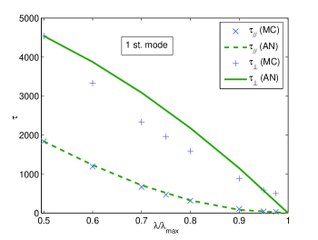
Figure 2: Monte-Carlo simulations of the first mode relaxation time for the perpendicular $\tau_{\perp}$ and parallel direction $\tau_{\parallel}$ (MC steps) as a function of relative degree of stretching $0.5<\lambda/\lambda_{max}<1$. Comparison with analytical (AN) and numerical results (MC).

The relevant feature here is that the relaxation time in both directions decreases as the chain is gradually stretched to its final limit. Evidently, the more stretched the chain is, the “stiffer” it becomes and, consequently, the relaxation time goes down. There is also a pronounced difference between the parallel and perpendicular relaxation times for the same $\lambda/\lambda_{max}$. The correlations in parallel direction decay faster (shorter relaxation time) than in perpendicular direction. However, this difference tends to disappear as the degree of stretching increased.

An important question concerns the degree to which the stretching affects the correlation between the first modes. In Figure 3 (a) and (b) we plot the autocorrelation $\langle X_{p\parallel,\perp}(0)^{2}\rangle$ and cross correlation $\langle X_{1\parallel,\perp}(0)X_{m\parallel,\perp}(0)\rangle$ functions as regards the mode number $m$ for different degrees of $\lambda/\lambda_{max}$. We want to emphasize two features. First, one should note that the power law of $\tau_{p\parallel,\perp}\propto p^{-1.98}$ is observed for all extensions and in both directions as this can be clearly seen from the insets of Fig. 3 (a) and (b). This behavior corresponds to our theoretical predictions and reflects the fact that the chain behaves like Gaussian at least as long as $0.5<\lambda/\lambda_{max}<0.975$.

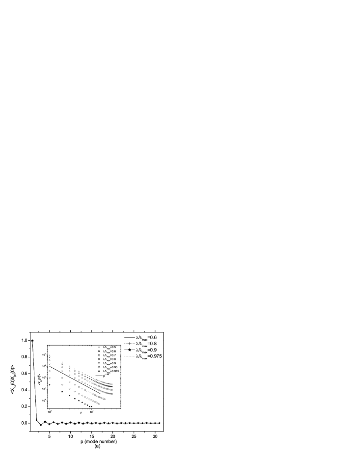
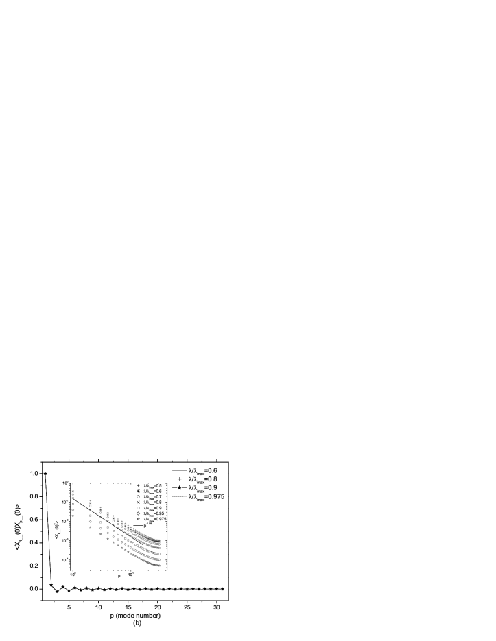
Figure 3: (a) $\langle X_{1\parallel}(0)X_{p\parallel}(0)\rangle$ against mode number $p$ for different relative extensions $\lambda/\lambda_{max}$. In the inset we plot the $p$ dependence of the function $\langle X_{p\parallel}(0)^{2}\rangle$, we show that the slope is almost equal to the predicted theoretical value $\propto p^{-2}$ (b) The same as in (a) for the perpendicular direction.

Figure 4: $\langle X_{1\parallel}(0)X_{p\perp}(0)\rangle$ as a function of the mode number $p$ for different extensions $\lambda/\lambda_{max}$.

Second, we find that the modes of the same direction seem to be orthogonal to each other for $1<p<31$, as in the linear (Rouse) case. For the cross correlation terms between different directions, $\langle X_{1\parallel}(0)X_{p\perp}(0)\rangle$, this is not the case at least for the lower modes $1<p<10$ which suggests that finite extensibility couples these modes in a certain way, see Fig. 4.

In conclusion, one may claim that this coupling effect, due to the nonlinearity of the interactions, seems to be stronger between modes of different directions and has apparently no effect on modes in the same direction. Generally, only the first modes ($1<p<10$) appear to couple since for modes with $p>10$ (that is, for short distance motions) the chain does not “feel” the fixed ends and the behavior is that of Rouse dynamics.

III.2 Molecular Dynamics results

Although real polymers do have mass, the inertia term is almost irrelevant as compared with the friction term, at least as long as the chain is not extended,. For high extensions, however, due to the large accelerations that each monomer is subject to, the inertia term is comparable and even larger than the friction term and the whole chain behaves as a string under tension in which oscillations are no more overdamped.

In this section we check the relevance of the inertia term, which should be important at the high stretching limit, and examine its physical consequences. To this end we run Molecular Dynamics simulations in which the mass of each monomer is accounted for in the corresponding equations of motion. For the implementation of the method we employ a successful numerical scheme developed and proved earlier by Dimitrov et al.Dimitrov . The model is again that of a simple coarse-grained bead-spring chain, originally proposed by Kremer and Grest Grest , which has been widely and very successfully used for MD simulations of polymers in various contexts KB ; Kotel . Effective monomers along the chain are bound together by a combination of the FENE potential, Eq. (22), where $K=15$ and the maximum bond extension is $l_{max}=1.5\sigma$, and a Lennard-Jones potential, responsible for the excluded volume interaction between the monomers. $\sigma=1$ is the range parameter of this purely repulsive Lennard-Jones (LJ) potential which is truncated and shifted to zero in its minimum and acts between any pairs of monomers.

$$U_{LJ}({\bf r})=4\epsilon_{LJ}\left[(\sigma/{\bf r})^{12}-(\sigma/{\bf r})^{6}+1\right],{\bf r}\leq{\bf r}_{c}=2^{1/6}\sigma$$ (26)

The parameter $\epsilon_{LJ}$, characterizing the strength of this potential, is chosen unity. Molecular Dynamics (MD) simulations were performed using the standard Velocity-Verlet algorithm Allen , performing typically $1.5\times 10^{9}$ time steps with an integration time step $\delta t=0.01t_{0}$ where the MD time unit (t. u.) $t_{0}=(\sigma^{2}m/48\epsilon_{LJ})^{1/2}=1/\sqrt{48}$, choosing the monomer mass $m_{b}=1$. The temperature was held constant by means of a standard Langevin thermostat with a friction constant $\zeta_{0}=0.5$

III.2.1 MD Simulation results

To make a comparison between Monte-Carlo and Molecular Dynamics simulations, we study the same cases with the same polymer chain of length $N=32$. This time, $2^{8}$ MD steps in each program running have been performed.

Typical data for the time, equal-mode correlation functions $C_{pp}(t)=\langle X_{p\parallel,\perp}(t)X_{p\parallel,\perp}(0)\rangle$ are presented for a particular value of $\lambda/\lambda_{max}=0.83$ and for the mode $p=3$. Figures 5a and 5b confirm the importance of taking inertia into account, manifested by the oscillations observed in the correlation functions. In Fig. 5a, which corresponds to the mode in parallel direction, one can recognize at least three frequencies in the correlation function, exposed by smaller satellite peaks in the Fourier spectrum in the inset. This broad-band spectrum does not mean that only 3 frequencies are present in the correlation function. One may rather claim that a continuum of frequencies of decreasing amplitude appears instead, reflecting the fact that these frequencies are clearly discernable from their neighbor values. Apparently, this effect manifests itself less visibly for the perpendicular direction, at least for this value of $\lambda/\lambda_{max}$ where only one peak can be well distinguished (see Fig. 5b). This single frequency appearing in the correlation function allows us to consider it as a linear underdamped motion of the chain for this case.

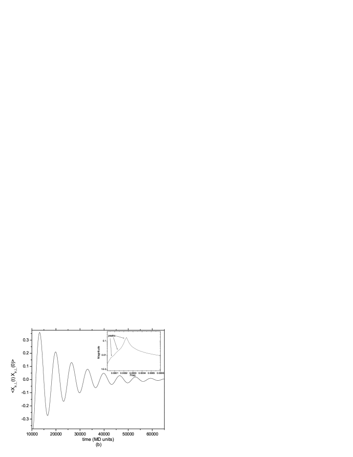
Figure 5: (a) $\langle X_{p\parallel}(t)X_{p\perp}(0)\rangle$ versus time (in MD time units) for $p=3$. In the inset the Fourier spectrum of the same function shows a sharp maximum, corresponding to the high basic frequency. Two smaller satellite peaks correspond to lower frequencies, also present in the mode dynamics. (b) The same as in (a) but in perpendicular direction. The Fourier spectrum reveals the presence of a single well-defined frequency in contrast of other two, less visible, smaller peaks.

At this stage we can ask for the physical meaning of these satellite peaks shown in the above figure. To answer this question, we plot together, in Figures 6a and 6b the Fourier spectra (frequencies) of several mode correlation functions at three different degrees of extension. The first five modes in parallel direction are shown in Fig. 6a for $\lambda/\lambda_{max}=0.512\;,0.704\;,0.953$. One can readily see that with growing stretching, $\lambda/\lambda_{max}$, a central peak, corresponding to a principal frequency of oscillation, is formed. However, this is not the case for $\lambda/\lambda_{max}=0.512$, where such a peak is absent and the mode dynamics is spread almost uniformly over frequencies lower that $10^{-4}$. In the other two cases $\lambda/\lambda_{max}=0.704\;,0.953$ this spreading disappears and narrower peaked functions come out, suggesting that the mode motion is realized essentially by means of a single frequency. Now, we claim attention to a particular feature of Figure 6a. Take for example the case $\lambda/\lambda_{max}=0.704$ for $p=1$. There, by a vertical line we demonstrate that the frequency corresponding to this mode ($p=1$) coincides exactly with the satellite frequency peaks which appear in the higher mode correlation functions. Looking deeper, we can see that this is not prerogative of the first mode and is observed also for $p>1$. It takes place for larger extensions too. Clearly, this shows that the satellite peaks are exactly the main frequencies of higher mode correlation functions. At the same time it indicates coupling of lower modes with higher ones which is accompanied by exchange of energy between them. Evidently, this coupling effect becomes more significant with growing mode number and, most notably, at lager extensions (see curves for $\lambda/\lambda_{max}=0.953$).

Figure 6b shows the same quantities for the modes in perpendicular direction. In this case the situation is similar whereby the satellite peaks indicate that coupling between the modes is effectively weaker, and may be observed at the largest extensions only.

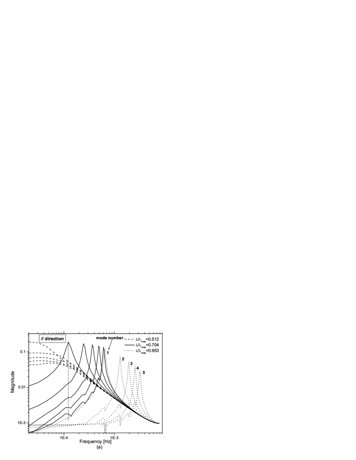
Figure 6: (a) Fourier spectra of correlation functions $\langle X_{p\parallel}(t)X_{p\parallel}(0)\rangle$ for the first $5$ modes in parallel direction at three degrees of relative extension $\lambda/\lambda_{max}$. The dash-dotted line is plotted as a guide to the eye. (b) The same as in (a) for the perpendicular direction.

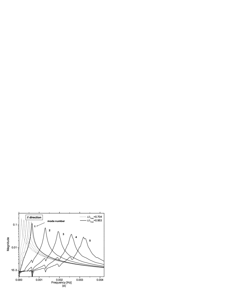
Figure 7: (a) Idem Figure 6, where a linear scale was used to show the broadening of the half-width of the main peak in the Fourier spectra of correlation functions $\langle X_{p\parallel}(t)X_{p\parallel}(0)\rangle$ for large values of $\lambda/\lambda_{max}=0.704\;0.953$. (b) The same as in (a) but this time the broadening if exists, does not appear to be significant.

More detailed information of the mode coupling effect can be extracted if one plots, for higher extensions $\lambda/\lambda_{max}=0.704\;,0.953$, the same functions as in Figure 6. This time, a normal scale in the frequency axes (abscissas) is employed to facilitate visualization. In Figure 7a, two significant effects can be well distinguished. On the one hand, we can appreciate a slight broadening of the half-width of the main peak with increasing extension for the same mode. On the other hand, a similar broadening occurs with increasing mode number, but this time at constant extension. Also the height of the main peak decreases with growing $p$. From a physical viewpoint, a broad-band spectra centered in a given frequency is associated with a continuum of frequencies (as mentioned above) around this single value. Returning to our problem, this means that as soon as we increase extension, more and more frequencies appear to make larger contributions in the dynamics of single mode correlation functions. A distinct situation accounts for the perpendicular direction. Noticeably, this broadening is not seen in Figure7b, and the peak height remains constant as one may verify from the similar graph depicted.

It is interesting to analyze the behavior of the principal frequency $\omega$, corresponding to the peak in the Fourier spectrum regarding the polymer chain extension.

In Figure 8a we demonstrate that the characteristic frequency in parallel direction $\omega_{\parallel}$ grows with increasing extension. At fixed value of the elongation $\lambda/\lambda_{max}$, $\omega_{\parallel}$ systematically increases with growing mode number $p$. For a special value of $\lambda/\lambda_{max}\approx 0.64$, however, one observes a local maximum in $\omega_{\parallel}$ which becomes increasingly pronounced as the mode number $p$ increases. In the inset to Figure 8a, where we show the variation of the relaxation times $\tau_{p}$ of the modes with changing elongation $\lambda/\lambda_{max}$, the region around $\lambda/\lambda_{max}\approx 0.64$ marks the end of the steady decrease of $\tau_{p}$ with growing degree of stretching. Thus, it appears that at some threshold extension $\lambda/\lambda_{max}\approx 0.64$ the chain dynamics undergoes a qualitative transition from an overdamped motion, determined essentially by friction, to ballistic motion governed by inertial effects.

In the overdamped regime the MD results are qualitatively consistent with the analytical predictions and MC data, indicating a clear decay of the relaxation times with increased stretching. Beyond some critical stretching, however, the dynamics changes and the polymer chain behaves increasingly like a string under tension. Then oscillations rather than random displacements of the monomers become important and the relaxation times of the different modes start to increase once again over a short range of chain elongations. Upon further stretching these relaxation times stay nearly constant. Eventually, in a regime of very strong stretching for $\lambda/\lambda_{max}>0.8$ the system becomes strongly nonlinear in nature and it becomes difficult to determine a well defined single “relaxation time”.

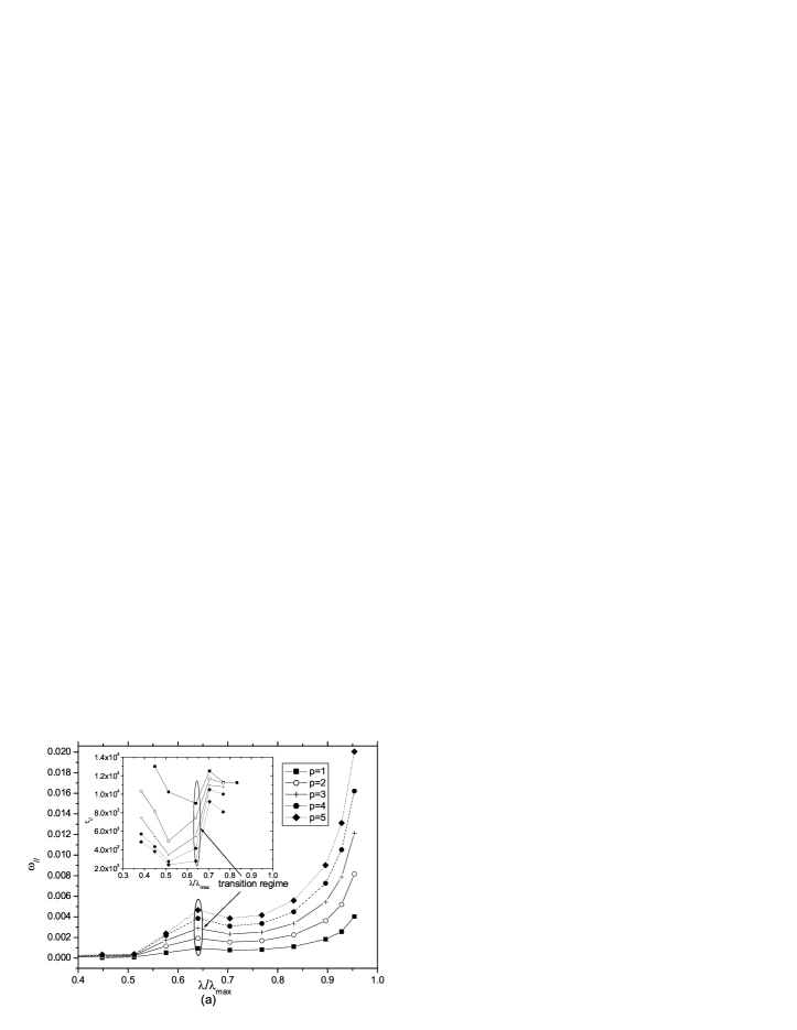
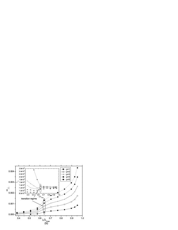
Figure 8: (a) Fourier spectrum of parallel mode correlation functions, $\langle X_{p\parallel}(t)X_{q\parallel}(0)\rangle$ against chain extension. In the inset one shows the variation of relaxation times $\tau_{p}$ for the first five modes with chain elongation $\lambda/\lambda_{max}$. (b) The same as in (a) for the perpendicular direction.

Figure 8b shows similar plots for the perpendicular direction. Rather than a maximum, the threshold position at $\lambda/\lambda_{max}\approx 0.64$ marks the onset of a stepper increase of the main frequency $\omega_{\perp}$ with growing elongation whereby at $\lambda/\lambda_{max}\rightarrow 1$ this frequency appears to diverge $\omega_{\perp}\rightarrow\infty$! The relaxation times $\tau_{\perp}$ of the various modes in perpendicular direction behave differently as compared to their counterparts of Fig. 8a. While in the overdamped regime at $\lambda/\lambda_{max}<0.64$ they decay steadily with growing elongation, in the inertial regime here after the threshold they merge to a nearly single value which remains largely unchanged for $\lambda/\lambda_{max}>0.64$. Remarkably, since the oscillations of the string in perpendicular direction persist up to very large extensions, $\lambda/\lambda_{max}\approx 1$, a well defined relaxation time can be found.

III.2.2 Approximate analytical model

It is possible to explain the observed behavior of the principal frequencies in the Fourier spectra of the mode-mode correlation functions as well as that of the relaxation times if one considers the linearized equations of motion (7). The intention here is to capture the essential features of the main frequencies $\omega_{\parallel,\perp}$ dependence on mode number $p$ and understand the insensitivity of the relaxation times with regard to chain elongation.

Our model of a chain pulled by force $f$ and fixed at the origin allow us to think of the chain as being fixed in space with elongation $\bar{R}_{\parallel}(N)$. One can then write an approximate equation of motion for ${\bf R}(s,t)$ using the information provided by the GSC method of section II.

First, we will decompose the position vector as ${\bf R}(s,t)=\widehat{{\bf R}}(s,t)+\langle{\bf R}(s,t)\rangle$, where $\widehat{{\bf R}}(s,t)$ is a new vector measuring the deviations of the position vector from its average position $\langle{\bf R}(s,t)\rangle$. Then, making use of previously defined quantities and expression (1), we can propose the following linearized equations

$$m_{b}\left\langle\frac{\partial^{2}R_{j}(s,t)}{\partial t^{2}}\right\rangle+\xi_{0}\left\langle\frac{\partial R_{j}(s,t)}{\partial t}\right\rangle-K_{j}\left\langle\frac{\partial^{2}R_{j}(s,t)}{\partial s^{2}}\right\rangle-f\delta_{sN}\delta_{jz}=0\hskip 36.135ptj=x,\;y,\;z$$ (27)

where we have replaced the exact force by a linearized (approximate) elastic force with elastic constants $K_{j}=K_{\parallel},K_{\perp}$, obtained in section II.2

$$\left[\left\langle\frac{\delta V[{\bf R}(s,t)-{\bf R}(s-1,t)]}{\delta R_{\parallel,\perp}(s,t)}\right\rangle+\left\langle\frac{\delta V[{\bf R}(s,t)-{\bf R}(s+1,t)]}{\delta R_{\parallel,\perp}(s,t)}\right\rangle\right]\approx K_{\parallel,\perp}\left\langle\frac{\partial^{2}R_{\parallel,\perp}(s,t)}{\partial s^{2}}\right\rangle$$ (28)

Separating the problem in the parallel and perpendicular direction as before and using the previously defined decomposition of vector ${\bf R}(s,t)$, since equations (27) are linear, we finally arrive at

$$m_{b}\left\langle\frac{\partial^{2}\widehat{R}_{\parallel,\perp}(s,t)}{\partial t^{2}}\right\rangle+\xi_{0}\left\langle\frac{\partial\widehat{R}_{\parallel,\perp}(s,t)}{\partial t}\right\rangle-K_{\parallel,\perp}\left\langle\frac{\partial^{2}\widehat{R}_{\parallel,\perp}(s,t)}{\partial s^{2}}\right\rangle=0$$ (29)

Introducing the Fourier expansion for $\langle\widehat{R}_{\parallel,\perp}(s,t)\rangle=\sum_{p}\langle\widehat{X}_{p\parallel,\perp}(t)\rangle\sin\left(\frac{p\pi s}{N}\right)$ and inserting it in (29), we obtain after multiplying it by $\widehat{X}_{p\parallel,\perp}(0)$

$$\sum_{p}\left(m_{b}\ddot{\widehat{C}}_{p\parallel,\perp}(t)+\xi_{0}\dot{\widehat{C}}_{p\parallel,\perp}(t)+K_{\parallel,\perp}\left(\frac{p\pi}{N}\right)^{2}\widehat{C}_{p\parallel,\perp}(t)\right)\sin\left(\frac{p\pi n}{N}\right)=0$$ (30)

where $\dot{\widehat{C}}_{p\parallel,\perp}(t)\equiv d\widehat{C}_{p\parallel,\perp}(t)/dt$ and $\widehat{C}_{p\parallel,\perp}(t)=\langle\widehat{{X}}_{p\parallel,\perp}(t)\widehat{{X}}_{p\parallel,\perp}(0)\rangle$. To satisfy (30), we require that

$$m_{b}\ddot{\widehat{C}}_{p\parallel,\perp}+\xi_{0}\dot{\widehat{C}}_{p\parallel,\perp}+K_{\parallel,\perp}\left(\frac{p\pi}{N}\right)^{2}\widehat{{C}}_{p\parallel,\perp}=0$$ (31)

Assuming that $\widehat{C}_{p\parallel,\perp}(t)=C_{p\parallel,\perp}^{0}\exp{(-\gamma_{p\parallel,\perp}t)}$, we finally obtain the eigenvalues of the linearized problem

$$\gamma_{p\parallel,\perp}=\frac{\xi_{0}}{2m_{b}}\pm\sqrt{\frac{\xi_{0}^{2}}{4m_{b}^{2}}-\frac{K_{\parallel,\perp}}{m_{b}}\left(\frac{p\pi}{N}\right)^{2}}$$ (32)

Clearly, these eigenvalues are real, showing a purely exponential decay, or complex, indicating damped oscillations, depending on the value of the radical in (32). Hence, these cases must be treated separately.

• Overdamped case

In this case, the radical is real, provided

$$\left(\frac{\xi_{0}}{2m_{b}}\right)^{2}>\frac{K_{\parallel,\perp}}{m_{b}}\left(\frac{p\pi}{N}\right)^{2}$$ (33)

and it is possible to identify $\gamma_{p\parallel,\perp}$ with the inverse of the relaxation time $\gamma_{p\parallel,\perp}=1/\tau_{p\parallel,\perp}$.

Returning to (32) and retaining only the first term in the Taylor expansion of the radical, $\sqrt{1-x^{2}}\approx 1-\frac{1}{2}x^{2}$, we find two values of $\gamma_{p\parallel,\perp}$ or $\tau_{p\parallel,\perp}$:

$$\frac{1}{\tau_{p\parallel,\perp}^{(1)}}\approx\frac{K_{\parallel,\perp}}{\xi_{0}}\left(\frac{p\pi}{N}\right)^{2}\hskip 14.45377pt\text{and}\hskip 14.45377pt\frac{1}{\tau_{p\parallel,\perp}^{(2)}}\approx\frac{\xi_{0}}{m_{b}}-\frac{K_{\parallel,\perp}}{\xi_{0}}\left(\frac{p\pi}{N}\right)^{2}$$ (34)

since eq. (31) is of second order in time. Evidently, to recover the theoretical result of section II for the relaxation time $\tau_{p\parallel,\perp}$, one must neglect the inertia term (inserting, for example, $m_{b}=0$) in (27) whereby only $\tau_{p\parallel,\perp}^{(1)}$ survives.

• Underdamped case

In this case the radical is negative,

$$\left(\frac{\xi_{0}}{2m_{b}}\right)^{2}<\frac{K_{\parallel,\perp}}{m_{b}}\left(\frac{p\pi}{N}\right)^{2}$$ (35)

Now, $\gamma_{p\parallel,\perp}$’s are complex quantities meaning that $\widehat{C}_{p\parallel,\perp}(t)$ corresponds to damped oscillatory motion. Clearly, the real part of $\gamma_{p\parallel,\perp}$ describes the degree of damping and the imaginary one gives the oscillation frequency which can be called $\omega_{p\parallel,\perp}$. If we still consider the real part of $\gamma_{p\parallel,\perp}$ as the inverse of a new relaxation time $\tau_{p\parallel,\perp}^{u}$ for the underdamped case, we find that $\gamma_{p\parallel,\perp}$ is equal to

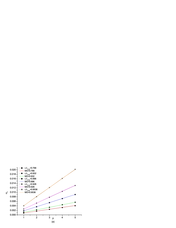
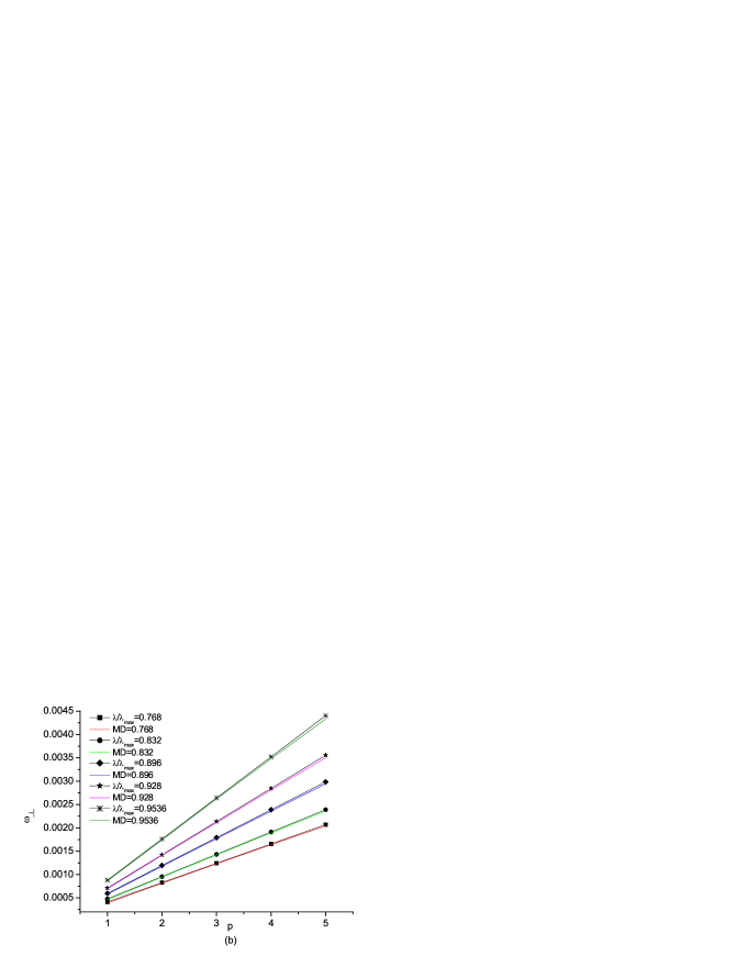
Figure 9: (a) Main frequency of the parallel mode correlation function $\omega_{p\parallel}$ as a function of mode number $p$ for different extensions in the underdamped regime. In the legend $\lambda/\lambda_{max}$ means analytical approximation, MD , Molecular dynamics simulations. (b) The same as in (a) in the perpendicular direction.

$$\gamma_{p\parallel,\perp}=\frac{1}{\tau_{p\parallel,\perp}^{u}}\pm i\omega_{p\parallel,\perp}=\frac{\xi_{0}}{2m_{b}}\pm i\left(\frac{K_{\parallel,\perp}}{m_{b}}\right)^{1/2}\left(\frac{p\pi}{N}\right)\sqrt{1-\left(\frac{\xi_{0}}{2m_{b}}\right)^{2}\left(\frac{N}{p\pi}\right)^{2}\frac{m_{b}}{K_{\parallel,\perp}}}$$ (36)

where $i=\sqrt{-1}$ is the imaginary unit. This can be approximated for large $p$ or large extensions ($K_{\parallel,\perp}\gg 1$) by

$$\frac{1}{\tau_{p\parallel,\perp}^{u}}=\frac{\xi_{0}}{2m_{b}}\hskip 14.45377pt\text{and}\hskip 14.45377pt\omega_{p\parallel,\perp}\approx\pm\left(\frac{K_{\parallel,\perp}}{m_{b}}\right)^{1/2}\left(\frac{p\pi}{N}\right)$$ (37)

where a Taylor expansion of the radical up to first order was carried out.

The last equation reveals some remarkable features. First of all, we can see a linear dependence on $p$ of the main frequencies in the mode correlation functions $\omega_{p\parallel,\perp}$. Secondly, an increasing of the magnitude of these frequencies upon increased stretching is also demonstrated. Figures 9a and b support these observations showing the reliability of the approximations. We plot $\omega_{p\parallel}$ 9a and $\omega_{p\perp}$ 9b against mode number $p$ for different extensions. Note that these findings apply only to the underdamped regime, $\lambda/\lambda_{max}>0.64$.

Moreover, a nearly constant relaxation time, $\tau_{p\parallel,\perp}^{u}$, which doesn’t depend on mode number or extension, comes out from equation (37) too. Upon qualitative comparison between Figures 8a and b (inset plots), we can conclude that for the perpendicular direction 8b, where a single relaxation time can be well defined even at very high extensions $\lambda/\lambda_{max}\approx 0.95$ the agreement is good. Instead, for the parallel direction 8a, a constant value of the relaxation time agrees with simulation results up to the extension where a single relaxation time can be well defined.

IV Conclusions

In the present paper we have studied the dynamics of a self-avoiding polymer chain at different degrees of stretching. Analytical work as well as computer simulations provide a rather consistent picture of the qualitative changes which the polymer dynamics undergoes upon gradual increase of the degree of stretching. In general, one observes two regimes of chain dynamics, depending on the degree of chain extension. In the first one, that of the friction dominated overdamped motion of the monomers, both analytic predictions as well as Monte Carlo results suggest a consistent picture of relaxation time decrease with growing stretching of the chain up to a threshold value $\lambda/\lambda_{max}\approx 0.64$ whereby the relaxation time parallel to stretching, $\tau_{||}$ is always considerably smaller (about one half) of that in direction perpendicular to stretching, $\tau_{\perp}$. For $\tau_{||}$ the agreement between analytic results from the GSC approximation and MC data is perfect on a quantitative level whereas for $\tau_{\perp}$ it is at most qualitative. As expected, the MC results for the relaxation time versus mode index relationship yield $\tau_{p}\propto p^{-2}$.

A transition regime at $\lambda/\lambda_{max}\approx 0.64$ where friction and inertia terms are of the same order of magnitude separates the overdamped regime from an inertial regime at higher degrees of stretching. This latter regime is strongly nonlinear in nature and a faithful description of the polymer dynamics can be produced by means of a MD simulation as well as by an approximate linearized analytical model.

Among the most salient features of polymer dynamics in this second regime of strong stretching, we find that normal modes are coupled to each other and can interchange energy, as expected in a system with strongly anharmonic interactions. These anharmonic contributions to the bond (FENE)-potential come into play at strong stretching only whereas in a weakly extended chain the monomers make the bonds oscillate around the equilibrium bond length by means of nearly harmonic forces and the modes are largely independent.

The Fourier analysis reveals the existence of principal characteristic frequencies of oscillatory motion for each normal mode. Along with this feature, a broad-band spectrum suggest the existence of a continuum of frequencies around the single peaks, which apparently make a non-vanishing contribution to the total motion. These principal characteristic frequencies have been shown by an approximate linear analytical model to scale linearly with mode index $p$. The frequencies also grow upon extension, as expected. A slight broadening of the half-width of the main frequency peak with increasing extension as well as with increasing mode number at constant extension, is revealed for the parallel direction. This means that as soon as we increase extension, more and more frequencies appear to contribute in the polymer dynamics, reflected by the single mode correlation functions. This broadening is not evidenced, at least up to $\lambda/\lambda_{max}=0.95$, for the perpendicular direction.

The relaxation times of the modes depend significantly on the considered direction. While in the parallel direction the relaxation times increase strongly in the transition region but then the possibility to define a single relaxation time for too large extensions $\lambda/\lambda_{max}>0.8$ becomes questionable, in the perpendicular direction the relaxation times remain more or less constants up to $\lambda/\lambda_{max}\approx 0.95$. It is remarkable that these results are also confirmed qualitatively by our linearized approach. Of course, one must keep in mind that such large extensions of a polymer chain might be of academic interest since bond rupture make take place if one approaches the tensile strength of the macromolecule.

V Acknowledgements

M. F. acknowledges the support and great hospitality of the Max Planck Institute for Polymer Research in Mainz, during his postdoctoral research position and also to the DFG FOR 597 for financial support. He also is indebted to Universidad Nacional del Sur and CONICET (Argentina) which gave him the possibility to make his postdoctoral studies. D.D. appreciates support from the Max Planck Institute of Polymer Research via MPG fellowship. A. M. and V.R. acknowledge support from the Deutsche Forschungsgemeinschaft (DFG), grant No. SFB 625/B4.

Appendix A

In calculating terms like $\left\langle\frac{\delta V[{\bf R}(s,t)-{\bf R}(s-1,t)]}{\delta R_{\parallel}(s,t)}\right\rangle$ one needs to tackle the term $\langle\delta[{\bf R}(s,t)-{\bf R}(s-1,t)-r]\rangle$ - see Section II.1. To this end we make the following approximation

$$\langle\delta[{\bf R}(s,t)-{\bf R}(s-1,t)-r]\rangle\approx\delta[\langle{\bf R}(s,t)-{\bf R}(s-1,t)-r\rangle].$$ (38)

Taking into account that $V(\vec{r})=-\frac{1}{2}k_{F}b_{0}^{2}\ln(1-\frac{\vec{r}^{2}}{b_{0}^{2}})$ and $\vec{r}^{2}=r_{\parallel}^{2}+r_{\perp}^{2}$, one can set

$$\int d^{3}r\langle\delta[{\bf R}(s,t)-{\bf R}(s-1,t)-r]\rangle\frac{\partial V(\vec{r})}{\partial r_{\parallel}}\approx k_{F}\frac{\bar{R}_{\parallel}(s,t)-\bar{R}_{\parallel}(s-1,t)}{1-\left[\frac{\bar{R}_{\parallel}(s,t)-\bar{R}_{\parallel}(s-1,t)}{b_{0}}\right]^{2}}$$

which is the final expression that must be inserted in the equation of motion.

The calculation of $A_{\parallel}(s,n,t)=C_{\parallel}(s,n,t)-\bar{R}_{\parallel}(s,t)\bar{R}_{\parallel}(n,t)$, proceeds as follows:

From equation (9) we have to calculate terms like $\left\langle R_{\parallel}(n,t)\frac{\delta V[{\bf R}(s,t)-{\bf R}(s-1,t)]}{\delta R_{\parallel}(s,t)}\right\rangle$. Using the $\delta$-function, one can write

$$\left\langle R_{\parallel}(n,t)\frac{\delta V[{\bf R}(s,t)-{\bf R}(s-1,t)]}{\delta R_{\parallel}(s,t)}\right\rangle=\left\langle R_{\parallel}(n,t)\int d^{3}r\langle\delta[{\bf R}(s,t)-{\bf R}(s-1,t)-r]\rangle\frac{\partial V(\vec{r})}{\partial r_{\parallel}}\right\rangle$$ (39)

Applying Wick’s theorem Wick we have

$$\left\langle R_{\parallel}(n,t)\frac{\delta V[{\bf R}(s,t)-{\bf R}(s-1,t)]}{\delta R_{\parallel}(s,t)}\right\rangle=\langle R_{\parallel}(n,t)\rangle\int d^{3}r\langle\delta[{\bf R}(s,t)-{\bf R}(s-1,t)-r]\rangle\frac{\partial V(\vec{r})}{\partial r_{\parallel}}+(\langle R_{\parallel}(n,t)R_{\parallel}(s,t)\rangle$$

$$-\langle R_{\parallel}(n,t)\rangle\langle R_{\parallel}(s,t)\rangle)\left\langle\frac{\delta}{\delta R_{\parallel}(s,t)}\int d^{3}r\delta[{\bf R}(s,t)-{\bf R}(s-1,t)-r]\frac{\partial V(\vec{r})}{\partial r_{\parallel}}\right\rangle+(\langle R_{\parallel}(n,t)R_{\parallel}(s-1,t)\rangle$$

$$-\langle R_{\parallel}(n,t)\rangle\langle R_{\parallel}(s-1,t)\rangle)\left\langle\frac{\delta}{\delta R_{\parallel}(s-1,t)}\int d^{3}r\delta[{\bf R}(s,t)-{\bf R}(s-1,t)-r]\frac{\partial V(\vec{r})}{\partial r_{\parallel}}\right\rangle$$

$$=\bar{R}_{\parallel}(n,t)\int d^{3}r\langle\delta[{\bf R}(s,t)-{\bf R}(s-1,t)-r]\rangle\frac{\partial V(\vec{r})}{\partial r_{\parallel}}+[A_{\parallel}(n,s,t)-A_{\parallel}(n,s-1,t)]\int d^{3}r\langle\delta[{\bf R}(s,t)-{\bf R}(s-1,t)-r]\rangle\frac{\partial^{2}V(\vec{r})}{\partial r_{\parallel}^{2}}$$

where the rhs was obtained after integrating by parts. For the term $\left\langle R_{\perp}(n,t)\frac{\delta V[{\bf R}(s,t)-{\bf R}(s-1,t)]}{\delta R_{\parallel}(s,t)}\right\rangle$, one has to replace the parallel variables by the perpendicular counterpart, taking into account that $\bar{R}_{\perp}(s)\equiv 0$.

Concerning the meaning of $K_{\parallel,\perp}(s,s\pm 1)$, we define an effective elastic constant:

$$K_{\parallel,\perp}(s,s\pm 1)=\int d^{3}r\langle\delta({\bf R}(s,t)-{\bf R}(s\pm 1,t)-r)\rangle\frac{\partial^{2}V(r)}{\partial r_{\parallel,\perp}^{2}}$$ (40)

Applying the same approximation as before, and after taking the second derivatives of the potential $V(r)$ with respect to perpendicular and parallel directions, we have for the perpendicular effective constant

$$K_{\perp}(s,s\pm 1)=k_{F}\frac{1}{1-\left[\frac{\bar{R}_{\parallel}(s,t)-\bar{R}_{\parallel}(s\pm 1,t)}{b_{0}}\right]^{2}}$$ (41)

and for the parallel one

$$K_{\parallel}(s,s\pm 1)=k_{F}\frac{1+\left[\frac{\bar{R}_{\parallel}(s,t)-\bar{R}_{\parallel}(s\pm 1,t)}{b_{0}}\right]^{2}}{\left(1-\left[\frac{\bar{R}_{\parallel}(s,t)-\bar{R}_{\parallel}(s\pm 1,t)}{b_{0}}\right]^{2}\right)^{2}}$$ (42)

The expression for the term $\langle R_{\perp}(n,t)h_{\perp}(s,t)\rangle$ can also be calculated by making use of the generalized Wick’s theorem Wick :

$$\langle R_{\parallel,\perp}(n,t)h_{\parallel,\perp}(s,t)\rangle=2\xi_{0}k_{B}T\left\langle\frac{\delta R_{\parallel,\perp}(n,t)}{\delta h_{\parallel,\perp}(s,t)}\right\rangle$$ (43)

As can be seen in Wick , the term $\left\langle\frac{\delta R_{\parallel,\perp}(n,t)}{\delta h_{\parallel,\perp}(s,t)}\right\rangle=\frac{1}{2\xi_{0}}\delta_{ns}$ so that the previous term gives

$$\langle R_{\parallel,\perp}(n,t)h_{\parallel,\perp}(s,t)\rangle=\delta_{ns}k_{B}T$$ (44)

References

- (1) P. E. Rouse, J. Chem. Phys. 21, 7 ( 1953)
- (2) P. Pincus, Macromolecules 10, 210 (1977).
- (3) P. G. De Gennes, Scaling Laws in Polymer Physics (Cornell University Press, Ithaca, NY, 1979).
- (4) Y. Marciano and F. Brochard-Wyart, Macromolecules 28, 985 (1995).
- (5) J. W. Hatfield and S. R. Quake, Phys. Rev. Lett. 82 3548 (1999).
- (6) J. J. C. Busfield, A. G. Thomas, and M. F. Ngah, Proceedings of the First European Conference on Constitutive Models for Rubber, Vienna, 1999.
- (7) M. E. Gurtin, Configurational Forces as Basic Concept of Continuum Physics (Springer Verlag, New York, 2000).
- (8) D. Gross and T. Seelig. Bruchmechanik mit einer Einf hrung in die Mikromechanik (Springer Verlag, Berlin, 2001).
- (9) D. Gross, R. M ller, and S. Kolling. Mechanics Research Communications 29, 529 (2002).
- (10) P. Haupt and A. Lion, Continuum Mechanics and Thermodynamics 7, 73 (1995).
- (11) B. N. J. Persson, O. Albohr, G. Heinrich, and H. Ueba, On tear and wear strength of rubber-line materials, preprint, 2008.
- (12) G. R. Hamed, Rubber Chem. Technol 67, 529 (1994).
- (13) M. Doi and S. F. Edwards, The theory of Polymer Dynamics( Oxford Science Publications, 1986)
- (14) E. G. Timoshenko, Yu. A. Kuznetsov, and K. A. Dawson, J. Chem. Phys. 102, 4 (1995).
- (15) N. Attig and K. Kremer, Computational soft matter: from sinthetic polymers to proteins (John von Neumann Institute for Computing, NIC Series, Vol. 23, 2004).
- (16) P. M. Morse and H. Feshbach, Methods of Theoretical Physics ( McGraw-Hill, New York, Part I, 1953)
- (17) A. Corsi, A. Milchev, V. G. Rostiashvili, and T. A. Vilgis, Macromolecules 39 1234 (2006).
- (18) D. I. Dimitrov, A. Milchev and K. Binder, Phys. Rev. Lett. 99, 54501 (2007).
- (19) G. S. Grest and K. Kremer, Phys. Rev. A 33, 3628 (1986).
- (20) K. Binder Monte Carlo and Molecular Dynamics Simulations in Polymer Science (Oxford Univ. Press, N.Y., 1995).
- (21) M. Kotelyanskii and D. N. Theodoru, Computer Simulation Methods for Polymers (M. Dekker, N.Y., 2004).
- (22) M. P. Allen and D. J. Tildesley, Computer Simulations of Liquids (Clarendon Press, Oxford, 1987).
- (23) J. Zinn-Justin, Quantum field theory and critical phenomena (Oxford Science Publications, Section 4.2., 1993)