Ricci flows, wormholes and critical phenomena

Abstract

We study the evolution of wormhole geometries under Ricci flow using numerical methods. Depending on values of initial data parameters, wormhole throats either pinch off or evolve to a monotonically growing state. The transition between these two behaviors exhibits a from of critical phenomena reminiscent of that observed in gravitational collapse. Similar results are obtained for initial data that describe space bubbles attached to asymptotically flat regions. Our numerical methods are applicable to “matter-coupled” Ricci flows derived from conformal invariance in string theory.

1 Introduction

An analog of the diffusion equation for geometries is the so-called Ricci flow. This is a type of parabolic partial differential equation that homogenizes geometry in a manner similar to the homogenization of density or heat produced by the diffusion equation.

The Ricci flow equation was first studied in the early 1980s. It arose nearly simultaneously in mathematics [1], in the study of the classification of 3-geometries, and in string theory physics [2, 3] from the requirement that a quantized string retain conformal invariance. Certain modifications of the purely geometric flow equation by “matter terms” motivated by string theory were central to Perelman’s [4] work on the Poincare conjecture.

A goal of analytic work on the flow equations is to study the approach to singularities, and to understand the so-called “ancient solutions,” which are the non-linear analogs of the heat kernel of the diffusion equation. Much of the work in this area has focused on the flow of compact geometries [5], with relatively little on non-compact cases such as the asymptotically flat or anti-deSitter geometries. In the asymptotically flat case for dimension $n\geq 3$, it has been demonstrated recently that the flow exists and remains asymptotically flat for an interval of time, with the mass remaining constant [6, 7]. For the rotationally symmetric case, Ref. [6] also shows that the flow is eternal for data containing no minimal surfaces.

The purpose of this paper is to investigate numerically some examples of the flow of asymptotically flat geometries, and to describe techniques that are easy to generalize to cases where matter flow equations are included.

Previous numerical work on Ricci flows focused on the (compact) case of a 3-sphere that is corseted (i.e., a surface formed by uniformly shrinking the equator of a 3-sphere), where it was found that the manifold flows to a round 3-sphere or a neck pinch depending on the degree of corseting [8]. The flow of horizon area and Hawking mass has also been studied [9] for initial data that is viewed as time symmetric data for the Einstein constraint equations. Numerical work pertaining to string theory aims at obtaining new black hole solutions as fixed points [10].

The focus of the present work is the geometric flow of wormhole geometries. We study several classes of initial data and find two possible outcomes: the wormhole “pinches off” leaving two disjoint asymptotically flat regions, or it expands indefinitely. We also find that there is a type of critical behaviour that separates these extreme cases. The numerical methods we utilize are stable for long time flows, and have potential applicability to the largely unexplored geometry-matter cases.

2 Flow equations

The Hamilton-DeTurck Ricci flow is defined by the equation [1, 11]

$$\partial_{t}g_{ab}=-2R_{ab}+2\nabla_{(a}V_{b)}.$$ (1)

For our work, we take $g_{ab}=g_{ab}(t,x^{c})$ to be the 3-metric on a manifold $\Sigma_{t}$ with Euclidean signature and $R_{ab}$ is the associated Ricci tensor. The parameter $t$ labels different 3-geometries along the flow and should not be confused with the intrinsic 3-dimensional coordinates $x^{c}$. Finally, $V^{a}$ is a DeTurck vector field that generates diffeomorphisms along the flow. The DeTurck field essentially represents the freedom to change 3-dimensional coordinates as the flow progresses. It is useful to note that $t$ has dimensions of $[\mathrm{length}]^{2}$ and $V^{a}$ has dimensions of $[\mathrm{length}]^{-1}$.

We assume the 3-manifolds $\Sigma_{t}$ are spherically symmetric, for which a general metric ansatz is

$$ds^{2}=e^{2X(t,\rho)}[d\rho^{2}+R^{2}(t,\rho)d\Omega^{2}].$$ (2)

Spherical symmetry implies the following form for the DeTurck field:

$$V^{a}=V(t,\rho)\partial_{\rho}.$$ (3)

When (2) and (3) are put into (1) we obtain two independent flow equations for $\partial_{t}X(t,\rho)$ and $\partial_{t}R(t,\rho)$. There is no dynamical equation for $V(t,\rho)$, so the system is underdetermined, which reflects the coordinate freedom embodied by the DeTurck field. To close the system, we need to fix coordinate gauges. There are three choices we have investigated:

1. $V(t,\rho)\equiv 0$;

2. $R(t,\rho)\equiv\rho$ (conformally flat gauge); or

3. $X(t,\rho)\equiv 0$ (areal radius gauge).

Enforcement of condition (2) or (3) in the flow equations (1) results in a single dynamical equation for $X(t,\rho)$ or $R(t,\rho)$, respectively, and an equation of constraint for $V(t,\rho)$. The choice (1) gives two dynamical equations for both metric functions.

For our purposes, a wormhole geometry is defined by a metric (2) that has two asymptotically flat regions as $\rho\rightarrow\pm\infty$. The combination $e^{X(t,\rho)}R(t,\rho)$ should be non-zero for all $\rho$, and the wormhole throat (or throats) are located at local minima $\rho=\rho_{\mathrm{th}}$ of this function

$$\partial_{\rho}(e^{X}R)\big{|}_{\rho=\rho_{\mathrm{th}}}=0,\quad\partial^{2}_{\rho}(e^{X}R)\big{|}_{\rho=\rho_{\mathrm{th}}}>0.$$ (4)

The definition of the wormhole throat suggests a convenient coordinate gauge choice is given by case (3) above, with line element

$$ds^{2}=d\rho^{2}+R^{2}(t,\rho)\,d\Omega^{2}.$$ (5)

In this gauge the area of 2-spheres of constant $\rho$ is $4\pi R^{2}(t,\rho)$, hence the name “areal radius” gauge. The condition $X\equiv 0$ reduces the flow equations (1) to

$$\partial_{t}R=\partial^{2}_{\rho}R+\frac{(\partial_{\rho}R)^{2}}{R}-\frac{1}{R}+V\partial_{\rho}R,$$ (6a)

$$\partial_{\rho}V=-2\frac{\partial_{\rho}^{2}R}{R}.$$ (6b)

As mentioned above, the latter is a constraint equation. These equations must be supplemented by boundary conditions and initial data. In the areal radius gauge, asymptotic flatness requires that

$$R\sim|\rho|+\mathcal{O}\left(l_{1}\ln\left(|\rho|/l_{2}\right)\right),$$ (6g)

where $l_{1}$ and $l_{2}$ are two length scales. Putting this asymptotic limit into (6a) and (6b), we obtain

$$V\sim\mathcal{O}\left(|\rho|^{-2}\right).$$ (6h)

The asymptotic behaviour of $R$ suggests that we search for solutions that are even functions of $\rho$. We then only need to consider the interval $\rho\in[0,\infty)$, and we have the additional boundary condition

$$\partial_{\rho}R\big{|}_{\rho=0}=0.$$ (6i)

The boundary conditions imply that there is always a local extrema of $R$ at $\rho=0$. If this is a minima, then there is a throat at $\rho=0$. To complete the specification of the flow, we need to give initial data for $R$ at $t=0$. The various classes of initial data considered in this work are described in §4 and §5.

Finally, we note that it is possible to embed the 3-geometries (5) in 4-dimensional flat space

$$ds^{2}=dR^{2}+dZ^{2}+R^{2}d\Omega^{2},$$ (6j)

via the parametric equations

$$R=R(t,\rho),\quad Z=Z(t,\rho),\quad\partial_{\rho}Z=\sqrt{1-(\partial_{\rho}R)^{2}}.$$ (6k)

These embeddings are only possible for areal radius functions satisfying $|\partial_{\rho}R|<1$. We use these as a tool for the visualization of Ricci flow initial data in Figs. 1 and 4.

3 Numerical method

We solve the equations (6a) and (6b) numerically using finite difference methods. The computational domain is defined by $\rho\in[0,\rho_{\mathrm{max}}]$ and $t\in[0,t_{\mathrm{max}}]$. The spatial and temporal intervals are discretized into elements of size $\delta\rho$ and $\delta t$, respectively. The notation $A_{i}^{j}$ refers to the value of the quantity $A(t,\rho)$ at the $i^{\mathrm{th}}$ spatial and $j^{\mathrm{th}}$ temporal node. The Neumann boundary condition (6i) is imposed explicitly, while the asymptotic boundary conditions (6g) and (6h) are replaced with the Dirichlet conditions

$$R(t,\rho_{\mathrm{max}})=R_{\mathrm{max}},\quad V(t,\rho_{\mathrm{max}})=0.$$ (6l)

$R_{\mathrm{max}}$ is fixed by the asymptotically flat initial data. With this, the former condition effectively gives $dR/d\rho\sim 1$ for large $\rho$ in our simulations, while the latter leads to a non-zero value of $V$ at the origin $\rho=0$. For $\rho_{\mathrm{max}}$ sufficiently large compared to $t_{\mathrm{max}}$, the simulation results are insensitive to the position of the outer boundary. In practice, our simulations are performed with $R_{\mathrm{max}}\sim\rho_{\mathrm{max}}\geq 200$.

The two types of finite differencing schemes used to approximate derivatives are summarized in Table 1. When applied to linear parabolic systems, the simple Euler (SE) method is known to be conditionally stable when $\delta t/\delta\rho^{2}\lesssim 1$. Conversely, the modified Dufort-Frankel (MDF) method is known to be unconditionally stable. Via direct experimentation, we have found that these conclusions also hold for the nonlinear problem given by equations (6a) and (6b), which would naïvely suggest that the MDF method is vastly superior to the SE method due to its excellent stability.

	Simple Euler (SE)	Modified Dufort-Frankel (MDF)
$\partial_{\rho}A$	$(A^{j}_{i+1}-A^{j}_{i-1})/(2\,\delta\rho)$	$(A^{j}_{i+1}-A^{j}_{i-1})/(2\,\delta\rho)$
$\partial^{2}_{\rho}R$ in eq. (6a)	$(R^{j}_{i+1}-2R^{j}_{i}+R^{j}_{i-1})/{\delta\rho^{2}}$	$(R^{j}_{i+1}-R^{j+1}_{i}-R^{j-1}_{i}+R^{j}_{i-1})/{\delta\rho^{2}}$
$\partial^{2}_{\rho}R$ in eq. (6b)	$(R^{j}_{i+1}-2R^{j}_{i}+R^{j}_{i-1})/{\delta\rho^{2}}$	$(R^{j}_{i+1}-2R^{j}_{i}+R^{j}_{i-1})/{\delta\rho^{2}}$
$\partial_{t}R$	$(R^{j+1}_{i}-R^{j}_{i})/\delta t$	$(R^{j+1}_{i}-R^{j-1}_{i})/(2\,\delta t)$
accuracy	$\mathcal{O}(\delta t,\delta\rho^{2})$	$\mathcal{O}(\delta t^{2},\delta\rho^{2})$

Table 1: Summary of the simple Euler (SE) and modified Dufort-Frankel (MDF) finite difference derivative approximations. In the top line, $A$ stands for either $R$ or $V$. Notice that for the MDF method, the second-order spatial derivative of $R$ is handled differently in the flow (6a) and constraint (6b) equations.

However, there is a non-trivial price to be paid for this attractive feature. One can show that the numerical results obtained with the MDF approximation actually converge to solutions of

$$\partial_{t}R=\partial^{2}_{\rho}R+\frac{(\partial_{\rho}R)^{2}}{R}-\frac{1}{R}+V\partial_{\rho}R-\left(\frac{\delta t}{\delta\rho}\right)^{2}\partial_{t}^{2}R,$$ (6m)

rather than the solutions of the original flow equation (6a). In other words, the MDF method solves a modified version of the original system of PDEs. In order to minimize the discrepancy between MDF results and the “true” solutions of (6a), one must make the ratio $\epsilon\equiv\delta t/\delta\rho$ as small as is computationally feasible.

The numerical results presented in this paper are obtained using the MDF method with $\epsilon=10^{-4}$. For several individual cases, we have checked that the simulation results are insensitive to the particular choice of $\delta t$ and $\delta\rho$ provided that $\epsilon\lesssim 10^{-3}$, and that the MDF and SE schemes give virtually identical answers for $\epsilon=10^{-4}$.

4 Evolution of Morris-Thorne wormhole geometries

The Morris-Thorne wormholes [12] have spatial sections

$$ds^{2}=\frac{1}{f(r)}dr^{2}+r^{2}d\Omega^{2},\quad f(r)=1-\frac{b(r)}{r}.$$ (6n)

In this section, we will use these metrics as initial data for the Ricci flow. At the initial time $t=0$, this 3-metric can be transformed into the areal radius gauge (5) by the coordinate transformation $r=R(0,\rho)$ with

$$\partial_{\rho}R(0,\rho)=\sqrt{f(R(0,\rho))},$$ (6o)

where $R(0,\rho)$ is the initial profile for the areal radius metric function. We will concentrate on a subset of this class defined by

$$b(r)=\frac{r_{0}^{\alpha}}{r^{\alpha-1}},\quad f(r)=1-\left(\frac{r_{0}}{r}\right)^{\alpha},$$ (6p)

where $r_{0}$ is a length scale and $\alpha$ is a dimensionless parameter (a similar family of wormholes was defined in [13]). The spatial sections of the Schwarzschild metric (known as the Einstein-Rosen bridge) correspond to $\alpha=1$. Another special case is the Ellis wormhole with $\alpha=2$ [14], which has $R(0,\rho)=\sqrt{\rho^{2}+r_{0}^{2}}$. Embedding diagrams of both types of wormholes appear in Figure 1. For Ricci flow of these wormholes, it is useful to work with dimensionless quantities defined by

$$\hat{\rho}=\rho/r_{0},\quad\hat{t}=t/r_{0}^{2},\quad\hat{R}\rightarrow R/r_{0},\quad\hat{V}\rightarrow r_{0}V.$$ (6q)

When the hatted-variables are substituted into the flow equations the $r_{0}$ length scale drops out of the problem; i.e., our simulation results are essentially independent of $r_{0}$ up to trivial scalings.

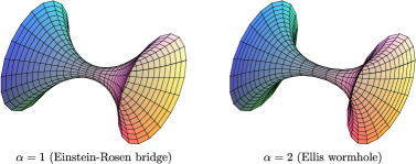
Figure 1: Embedding diagrams of the Einstein-Rosen and Ellis wormholes in flat space (we have set $\theta=\pi/2$ to obtain a 3-dimensional plot).

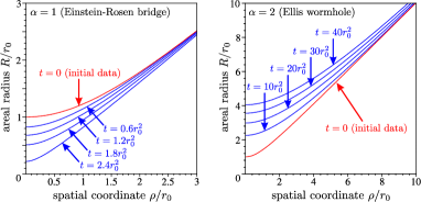
Figure 2: Evolution of the areal radius function $R(t,\rho)$ under the Ricci flow for Morris-Thorne wormhole initial data corresponding to $\alpha=1$ and $\alpha=2$. Note that our boundary conditions ensure that the wormhole throat is always at $\rho=0$ for these simulations.

In Figure 2, we show the results of our simulations for the evolution of the areal radius function $R(t,\rho)$ for the Einstein-Rosen and Ellis cases. One can see in Figure 1 that the initial data for the two scenarios are visually quite similar. However, the evolution of $R$ is entirely different: in the Ellis case the areal radius tends to diverge for all $\rho$ as $t\rightarrow\infty$, while for the Einstein-Rosen bridge $R$ is everywhere decreasing and the wormhole throat pinches off in finite time. Due to computing limitations, we cannot determine the ultimate fate of the Ellis initial data, but it appears to be a warped cylinder with a monotonically increasing radius.

In Figure 3, we plot the evolution of the throat radius $R_{\mathrm{th}}(t)=R(t,0)$ for various values of $\alpha$. We find that the wormhole throat pinches off for initial data with $\alpha$ less than a critical value $\alpha_{\mathrm{crit}}$. For cases with $\alpha>\alpha_{\mathrm{crit}}$, the throat approaches an ever-expanding state after a brief initial period of contraction. Numerically, we have determined the value of the critical parameter to be approximately 1.259. For $\alpha>\alpha_{\mathrm{crit}}$, the throat radius appears to grow like $\sqrt{t}$ at late times.

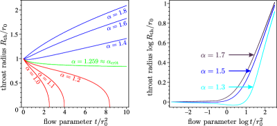
Figure 3: Ricci flow evolution of the throat radius $R_{\mathrm{th}}(t)=R(t,0)$ for various Morris-Thorne wormhole initial data.

5 Evolution of “bubble” geometries

A geometrically interesting question is: What does the Ricci flow evolution of a bubble attached to asymptotically flat space look like? In the areal radius gauge, initial data for this kind of problem would roughly be

$$R(0,\rho)\sim r_{0}\cases{\sin\rho/r_{0}&for $0\leq\rho\lesssim\rho_{0}$\\ \rho/r_{0}&for $\rho\gtrsim\rho_{0}$},$$ (6r)

where $\rho_{0}<\pi r_{0}$ is some transition radius. Notice that this initial data has $R=0$ and $\partial_{\rho}R\neq 0$ at $\rho=0$, so it violates the boundary conditions that our code was designed to deal with. We therefore consider the related problem of a bubble attached to two asymptotically flat regions, and leave initial data of the form (6r) for future work. We take initial data for the current problem to be

$$R(0,\rho)=\cases{r_{0}(1-\rho^{2}/r_{0}^{2})&for $|\rho|<\rho_{0}$\\ \sqrt{(|\rho|-\rho_{1})^{2}+\rho_{2}^{2}}&for $|\rho|\geq\rho_{0}$}.$$ (6s)

Here, $\rho_{1}$ and $\rho_{2}$ are selected such that both $R$ and $\partial_{\rho}R$ are continuous at the transition points $\rho=\pm\rho_{0}$. Defining the dimensionless parameter $\beta\equiv\rho_{0}/r_{0}$, we show embedding diagrams for two examples of this type of initial data in Figure 4. Note that there are two wormhole throats (local minima of $R$) in this case at $\rho=\pm\rho_{1}$, while there is a local maxima of $R$ at $\rho=0$. This maxima corresponds to the equator of our bubble, and it is easy to show that the ratio of the throat radii to the equator radius is

$${R_{\mathrm{th}}}/{R_{\mathrm{eq}}}=\rho_{2}/r_{0}=(1-\beta^{2})\sqrt{1-4\beta^{2}}.$$ (6t)

Hence, in order to have sensible initial data with $R>0$ we are obliged to take $0\leq\beta\leq 1/2$.

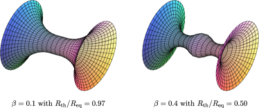
Figure 4: Embedding diagrams of 3-geometries representing a bubble connecting two asymptotically flat regions

Making use of the dimensionless quantities (6q), we have simulated the Ricci flow evolution of various types of bubble geometries. As in §4 above, we take $R$ to be an even function of $\rho$ and impose the boundary condition that $\partial_{\rho}R=0$ for $\rho=0$. We find that for $R_{\mathrm{th}}/R_{\mathrm{eq}}$ initially small, the bubbles disappear and the geometry “pinches-off” into a pair of disjoint asymptotically flat regions. For $R_{\mathrm{th}}/R_{\mathrm{eq}}$ initially close to unity, the bubbles also disappear and the areal radius blows up, somewhat similar to the $\alpha>\alpha_{\mathrm{crit}}$ cases in §4. Explicit examples of these behaviours are shown in Figure 5.

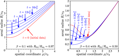
Figure 5: The evolution of two bubble geometries under the Ricci flow.

6 Conclusions

We have observed that the Ricci flow of certain families of rotationally symmetric wormhole geometries exhibit a form of critical behaviour: wormhole throats pinch off or expand forever depending on the values of initial data parameters. The expanding solutions are perhaps surprising at first sight, but are nevertheless understandable in that they appear to converge to an infinite volume cylindrical attractor.

This work complements both the analytic work on the flow of asymptotically flat geometries [6] and the numerical work on corsetted 3–spheres [8]. It would be of interest to see if the neck pinching seen in our simulations of wormhole throats may be modeled by the Bryant steady solitons, as has been observed for rotationally symmetric geometries on $S^{3}$ [15].

The methods we have used have applicability to a variety of situations for relevance to string theory, where the renormalization group flows give matter coupled modifications of Ricci flow. The interest here is in discovering new fixed points of physical relevance. For example, in special cases with compact target spaces and a tachyon field, there is evidence that properties of the tachyon potential are linked to the existence of non-trivial fixed points [16]. It is of interest to extend such cases to non-compact geometries with gauge or 2-form fields, and consider questions such as the possibility of stabilization of wormholes geometries.

Acknowledgements We would like to thank Eric Woolgar and Jack Gegenberg for discussions, David Hobill for suggesting that we try the Dufort-Frankel method, and David Garfinkle for comments on the manuscript. This work was supported by NSERC.

References

References

- [1] R. S. Hamilton, Three manifolds of Positive Ricci curvature, J. Diff. Geom. 17 255-306 (1982).
- [2] Friedan D 1980 Phys. Rev. Lett. 45 1057
- [3] Sen Ashoke 1985 Phys. Rev. D32 2102; 1985 Phys. Rev. Lett. 55 1846.
- [4] Perelman G 2003 math/0211159; math/0307245.
- [5] Cao H D and Chow B 1999 Recent developments on Ricci flow Bull. Am. Math. Soc. 36 59-74.
- [6] Oliynyk T and Woolgar E, Asymptotically Flat Ricci Flows, Commun. in Analysis and Geometry 15 (2007) 535–568; arXiv:math/0607438v2 [math.DG].
- [7] Dai X and Ma L Mass under the Ricci flow, arXiv:math/0510083v1 [math.DG].
- [8] Garfinkle D and Isenberg J 2002 Critical behaviour in Ricci flow arXiv: math/0306129v1 [math.DG].
- [9] Samuel J and Chowdhry S R 2008 Class. Quant. Grav. 25 035012.
- [10] Hedrick M and Wiseman T 2006 Class. Quant. Grav. 23 6683.
- [11] DeTurck D 1983 J. Differential Geom. 18 157.
- [12] Morris M and Thorne K S , Am. J. Phys. 56 395-412 (1988).
- [13] Lobo F (2005) Phys. Rev. D 71 084011
- [14] Ellis H G (1973) J. Math. Phys. 14 104
- [15] Garfinkle D and Isenberg J Modelling of Degenerate Neck Pinch Singularities in Ricci Flow by Bryant Solitons, arXiv: 0709.0514.
- [16] Gegenberg J and Suneeta V, JHEP 0609: 045, 2006; arXiv: hep-th/0605230.