Squeezed states produced by modulation interaction
and phase conjugation in fibers

1. Introduction

Parametric devices based on four-wave mixing (FWM) in fibers can generate photon pairs for quantum communication experiments [1, 2]. Three different types of FWM are illustrated in Fig. 1. Modulation interaction (MI) is the degenerate process in which two photons from the same pump are destroyed, and signal and idler (sideband) photons are created ($2\pi_{p}\rightarrow\pi_{s}+\pi_{i}$, where $\pi_{j}$ represents a photon with frequency $\omega_{j}$). Inverse MI is the degenerate process in which two photons from different pumps are destroyed and two signal photons are created ($\pi_{p}+\pi_{q}\rightarrow 2\pi_{s}$). Phase conjugation (PC) is the nondegenerate process in which two different pump photons are destroyed and two different sideband photons are created ($\pi_{p}+\pi_{q}\rightarrow\pi_{s}+\pi_{i}$). These processes are reviewed in [3, 4, 5, 6].

     

     

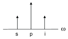
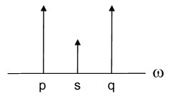
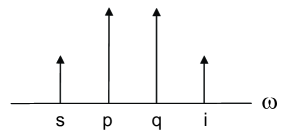
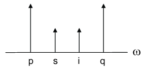
Figure 1: Frequency diagram for ($a$) modulation interaction, ($b$) inverse modulation interaction, ($c$) outer-band phase conjugation and ($d$) inner-band phase conjugation in a fiber. Long arrows denote strong pumps ($p$ and $q$), whereas short arrows denote weak sidebands ($s$ and $i$).

The evolution of an optical system is governed by the (spatial) Schrödinger equation

$$d_{z}|\psi\rangle=iH|\psi\rangle,$$ (1)

where $z$ is distance, $d_{z}=d/dz$, $|\psi\rangle$ is the state vector, and the Hamiltonian $H$ depends on the creation and destruction operators of the interacting modes ($a_{j}^{\dagger}$ and $a_{j}$, respectively, where $\dagger$ denotes a hermitian conjugate). The solution of Eq. (1) can be written in the input–output form

$$|\psi(z)\rangle=U(z)|\psi(0)\rangle,$$ (2)

where the evolution operator $U(z)=\exp(iHz)$ is unitary. Notice that $U(-z)=U^{\dagger}(z)$. In the Schrödinger picture, the mode operators are constants.

In the Heisenberg picture, one defines the mode operators $a_{j}(z)=U^{\dagger}(z)a_{j}(0)U(z)$, which evolve according to the (spatial) Heisenberg equations

$$d_{z}a_{j}=i[a_{j},H],$$ (3)

where $[\ ,\ ]$ denotes a commutator. In the small-signal (undepleted-pump) regime, the Hamiltonian depends quadratically on the sideband operators, so Eqs. (3) are linear in these operators. Hence, their solutions can be written in the input–output form

$$a_{j}(z)={\textstyle\sum}_{k}[\mu_{jk}(z)a_{k}(0)+\nu_{jk}(z)a_{k}^{\dagger}(0)],$$ (4)

where $\mu_{jk}(z)$ and $\nu_{jk}(z)$ are transfer functions.

Any measurable quantity associated with mode $j$ can be written as the expectation value of some function of the mode operator and its conjugate. Common examples are the field quadrature and photon number. Let $\langle\ \rangle$ denote an expectation value and $F$ be any function that has a Taylor expansion. Then

$$\langle F(a_{j})\rangle=\langle\psi(z)|F[a_{j}(0)]|\psi(z)\rangle=\langle\psi(0)|F[a_{j}(z)]|\psi(0)\rangle.$$ (5)

In the Schrödinger picture [first part of Eq. (5)], the state vector evolves and the mode operator is constant, whereas in the Heisenberg picture [second part of Eq. (5)] the state vector is constant and the mode operator evolves. Expectation values of output quantities (which involve one or more operators) can be calculated using either picture.

To model photon-generation experiments, one needs to determine the probabilities of measuring different numbers of photons. In this context, the Schrödinger picture is preferable. In this report, number-state expansions are derived for the squeezed states produced by (inverse) MI and PC in fibers. These expansions generalize the standard results [7, 8], which do not include the effects of fiber dispersion. As written, they apply to parametric processes driven by continuous-wave pumps. However, by defining suitable superposition (Schmidt) modes [9, 10], one can also apply them to parametric processes driven by pulsed pumps.

2. One-mode squeezed state

The inverse MI in a fiber is governed by the Hamiltonian

$$H=\delta a_{s}^{\dagger}a_{s}+[\gamma(a_{s}^{\dagger})^{2}+\gamma^{*}a_{s}^{2}]/2,$$ (6)

where $a_{s}$ is the destruction operator of the signal mode, $\delta$ is the mismatch coefficient and $\gamma$ is the coupling coefficient. Formulas for these coefficients, which involve the fiber dispersion and nonlinearity coefficients, and the the pump amplitudes, are stated in [4, 6].

By combining Eqs. (3) and (6), one obtains the evolution equation

$$d_{z}a_{s}=i\delta a_{s}+i\gamma a_{s}^{\dagger}.$$ (7)

The solution of this equation can be written in the input–output form

$$a_{s}(z)=\mu(z)a_{s}(0)+\nu(z)a_{s}^{\dagger}(0),$$ (8)

where the transfer functions

$$\mu(z) = \cos(kz)+i\delta\sin(kz)/k,$$ (9)

$$\nu(z) = i\gamma\sin(kz)/k$$ (10)

and the inverse-MI wavenumber $k=(\delta^{2}-|\gamma|^{2})^{1/2}$. Equations (9) and (10) are based on the assumption that $k$ is real (and the MI is stable). If $k=i\kappa$ is imaginary (and the MI is unstable), $\cos(kz)$ is replaced by $\cosh(\kappa z)$ and $\sin(kz)/k$ is replaced by $\sinh(\kappa z)/\kappa$. Notice that $\mu(-z)=\mu^{*}(z)$ and $\nu(-z)=-\nu(z)$. The transfer functions also satisfy the auxiliary equation

$$|\mu|^{2}-|\nu|^{2}=1.$$ (11)

By definition, the one-mode squeezed state produced by inverse MI is $U(z)|0\rangle$, where $U(z)=\exp(iHz)$ and $|0\rangle$ is the one-mode vacuum state. One can facilitate the calculation of the output state by rewriting $U$ in normally-ordered form. To do this, one writes

$$H=\gamma K_{+}+2\delta K_{3}+\gamma^{*}K_{-}-\delta/2,$$ (12)

where the operators

$$K_{+}=(a_{s}^{\dagger})^{2}/2,\ \ K_{-}=a_{s}^{2}/2,\ \ K_{3}=(a_{s}^{\dagger}a_{s}+a_{s}a_{s}^{\dagger})/4.$$ (13)

These operators satisfy the angular-momentum-like commutation relations $[K_{+},K_{-}]=-2K_{3}$ and $[K_{3},K_{\pm}]=\pm K_{\pm}$. By using a standard operator-ordering theorem, which is proved in the Appendix, one finds that

$$\exp(iHz)=\exp(\gamma_{+}K_{+})\exp(\gamma_{3}K_{3})\exp(\gamma_{-}K_{-}),$$ (14)

where the auxiliary functions

$$\gamma_{+}(z) = i\gamma\sin(kz)/[k\cos(kz)-i\delta\sin(kz)],$$ (15)

$$\gamma_{-}(z) = i\gamma^{*}\sin(kz)/[k\cos(kz)-i\delta\sin(kz)],$$ (16)

$$\gamma_{3}(z) = -2\log[\cos(kz)-i\delta\sin(kz)/k]$$ (17)

and the (inconsequential) phase factor $\exp(-i\delta z/2)$ was omitted. It follows from Eq. (14), and the identities $K_{\pm}^{\dagger}=K_{\mp}$ and $K_{3}^{\dagger}=K_{3}$, that $\gamma_{+}(-z)=\gamma_{-}^{*}(z)$, $\gamma_{-}(-z)=\gamma_{+}^{*}(z)$ and $\gamma_{3}(-z)=\gamma_{3}^{*}(z)$. The auxiliary functions satisfy these conditions. By comparing Eqs. (15)–(17) to Eqs. (9) and (10), one obtains the compact formulas

$$\gamma_{+}=\nu/\mu^{*},\ \ \gamma_{-}=-\nu^{*}/\mu^{*},\ \ \gamma_{3}=-2\log(\mu^{*}).$$ (18)

Hence, if the input is the vacuum state, the output is the squeezed state

$$|\psi\rangle={1\over(\mu^{*})^{1/2}}\sum_{n=0}^{\infty}\biggl{(}{\nu\over\mu^{*}}\biggr{)}^{n}{[(2n)!]^{1/2}\over 2^{n}n!}|2n\rangle,$$ (19)

where the basis vectors $|2n\rangle=(a_{s}^{\dagger})^{2n}|0\rangle/[(2n)!]^{1/2}$. Notice that each eigenstate contains an even number of photons.

For the special case in which $\delta=0$ (maximal exponential growth),

$$\mu=\cosh(|\gamma|z),\ \ \nu=i\gamma\sinh(|\gamma|z)/|\gamma|,\ \ \nu/\mu^{*}=i\gamma\tanh(|\gamma|z)/|\gamma|$$ (20)

and Eq. (19) reduces to the standard result [7, 8]. (To verify this statement, use the substitution $i\gamma z=-se^{i\theta}$.) For the complementary case in which $\delta=|\gamma|$ (transitional linear growth),

$$\mu=1+i|\gamma|z,\ \ \nu=i\gamma z,\ \ \nu/\mu^{*}=i\gamma z/(1-i|\gamma|z)$$ (21)

and Eq. (19) reduces to the result of [11]. (Use the substitution $|\gamma|z=z$.)

It is customary (and easy) to calculate the moments of $a^{\dagger}$ and $a$ using the Heisenberg picture. However, I will calculate the lower-order moments using the Schrödinger picture, to check Eq. (19) and illustrate its use. The zeroth-order moment is $\langle\psi|\psi\rangle$. Let $c_{n}$ be the coefficient of $|2n\rangle$ in Eq. (19) and $P_{2n}=|c_{n}|^{2}$ be the probability of a $2n$-photon state. Then $|\mu|P_{2n}=x^{2n}(2n)!/4^{n}(n!)^{2}$, where $x=|\nu/\mu|$. It follows from Eq. (11) and the identity

$$S(x)={1\over(1-x^{2})^{1/2}}=\sum_{n=0}^{\infty}{x^{2n}(2n)!\over 4^{n}(n!)^{2}}$$ (22)

that $\langle\psi|\psi\rangle=1$: The state vector (19) is normalized.

The field quadrature

$$q_{s}=(a_{s}^{\dagger}e^{i\phi_{l}}+a_{s}e^{-i\phi_{l}})/2^{1/2},$$ (23)

where $\phi_{l}$ is the local-oscillator phase, and the quadrature deviation $\delta q_{s}=q_{s}-\langle q_{s}\rangle$. The first-order moment

$$\langle q_{s}\rangle=0,$$ (24)

because $a^{\dagger}|\psi\rangle$ and $a|\psi\rangle$ contain only odd-number states, whereas $\langle\psi|$ contains only even-number states. The expectation values (means) of all the odd moments are zero, for the same reason. To calculate the quadrature variance $\langle\delta q_{s}^{2}\rangle$ (which equals $\langle q_{s}^{2}\rangle$), one needs to calculate the inner products of $\langle\psi|$ and

$$(a_{s}^{\dagger})^{2}|\psi\rangle = (\mu^{*}/\nu)\sum_{n=1}^{\infty}2nc_{n}|2n\rangle,$$ (25)

$$a_{s}^{\dagger}a_{s}|\psi\rangle = \sum_{n=1}^{\infty}2nc_{n}|2n\rangle,$$ (26)

$$a_{s}a_{s}^{\dagger}|\psi\rangle = \sum_{n=0}^{\infty}(2n+1)c_{n}|2n\rangle,$$ (27)

$$a_{s}^{2}|\psi\rangle = (\nu/\mu^{*})\sum_{n=0}^{\infty}(2n+1)c_{n}|2n\rangle.$$ (28)

It follows from Eq. (22) that

$$|\mu|\sum_{n=0}^{\infty}2nP_{n}=xd_{x}S(x)={x^{2}\over(1-x^{2})^{3/2}}.$$ (29)

By using this result and Eq. (11) to evaluate the inner products, one finds that $\langle(a_{s}^{\dagger})^{2}\rangle=\mu^{*}\nu^{*}$, $\langle a_{s}^{\dagger}a_{s}\rangle=|\nu|^{2}$, $\langle a_{s}a_{s}^{\dagger}\rangle=|\mu|^{2}$ and $\langle a_{s}^{2}\rangle=\mu\nu$. Hence, the quadrature variance

$$\langle\delta q_{s}^{2}\rangle=(|\mu|^{2}+2|\mu\nu|\cos\theta+|\nu|^{2})/2,$$ (30)

where the phase difference $\theta=\phi_{\mu}+\phi_{\nu}-2\phi_{l}$. The quadrature variance attains its maximum $(|\mu|+|\nu|)^{2}/2$ when $\theta=0$ and its minimum $(|\mu|-|\nu|)^{2}/2$ when $\theta=\pi$. In the stable regime $|\nu|^{2}$ is bounded by $\gamma^{2}/k^{2}$, whereas in the unstable regime it is unbounded [Eq. (10)]. The quadrature is squeezed in both regimes. Equation (30) is consistent with the results of [6, 12], which were obtained using the Heisenberg picture. For the special case in which $\delta=0$, it reduces to the standard result [7, 8].

Now define the photon-number operator $n_{s}=a_{s}^{\dagger}a_{s}$ and the number deviation $\delta n_{s}=n_{s}-\langle n_{s}\rangle$. It also follows from Eq. (22) that

$$|\mu|\langle n_{s}^{m}\rangle=(xd_{x})^{m}S(x).$$ (31)

By using this result and Eq. (11), one finds that

$$\langle n_{s}\rangle=|\nu|^{2},\ \ \langle n_{s}^{2}\rangle=|\nu|^{2}(2|\mu|^{2}+|\nu|^{2}),\ \ \langle\delta n_{s}^{2}\rangle=2|\mu\nu|^{2}.$$ (32)

Equations (32) are consistent with the results of [6, 12], which were obtained using the Heisenberg picture. For the special case in which $\delta=0$, they reduce to the standard results [7, 8].

3. Two-mode squeezed state

MI and PC in a fiber are governed by the Hamiltonian

$$H=\delta(a_{s}^{\dagger}a_{s}+a_{i}^{\dagger}a_{i})+\gamma a_{s}^{\dagger}a_{i}^{\dagger}+\gamma^{*}a_{s}a_{i},$$ (33)

where $a_{j}$ is the destruction operator of mode $j$ ($s$ or $i$). Formulas for the mismatch and coupling coefficients are stated in [3, 5]. By combining Eqs. (3) and (33), one obtains the evolution equations

$$d_{z}a_{s} = i\delta a_{s}+i\gamma a_{i}^{\dagger},$$ (34)

$$d_{z}a_{i}^{\dagger} = -i\gamma^{*}a_{s}-i\delta a_{i}^{\dagger}.$$ (35)

The solutions of these equations can be written in the input–output form

$$a_{s}(z) = \mu(z)a_{s}(0)+\nu(z)a_{i}^{\dagger}(0),$$ (36)

$$a_{i}^{\dagger}(z) = \nu^{*}(z)a_{s}(0)+\mu^{*}(z)a_{i}^{\dagger}(0),$$ (37)

where the transfer functions were defined in Eqs. (9) and (10), and the MI (PC) wavenumber $k=(\delta^{2}-|\gamma|^{2})^{1/2}$.

By definition, the two-mode squeezed state produced by MI (PC) is $U(z)|0,0\rangle$, where $|0,0\rangle$ is the two-mode vacuum state. One can calculate this state by writing

$$H=\gamma K_{+}+2\delta K_{3}+\gamma^{*}K_{-}-\delta,$$ (38)

where the operators

$$K_{+}=a_{s}^{\dagger}a_{i}^{\dagger},\ \ K_{-}=a_{s}a_{i},\ \ K_{3}=(a_{s}^{\dagger}a_{i}+a_{s}a_{i}^{\dagger})/2.$$ (39)

These operators also satisfy the commutation relations $[K_{+},K_{-}]=-2K_{3}$ and $[K_{3},K_{\pm}]=\pm K_{\pm}$. By using the aforementioned operator-ordering theorem, one can rewrite $U$ in the form of Eq. (14), where the auxiliary functions were defined in Eqs. (15)–(17) and the (inconsequential) phase factor $\exp(-i\delta z)$ was omitted. Hence, if the input is the vacuum state, the output is the squeezed state

$$|\psi\rangle={1\over\mu^{*}}\sum_{n=0}^{\infty}\biggl{(}{\nu\over\mu^{*}}\biggr{)}^{n}|n,n\rangle.$$ (40)

Notice that each eigenstate contains an equal number of signal and idler photons. For the special cases in which $\delta=0$ and $\delta=|\gamma|$, Eq. (40) reduces to the standard result [7, 8] and the result of [11], respectively.

Let $c_{n}$ be the coefficient of $|n,n\rangle$ in Eq. (40) and let $P_{n}=|c_{n}^{2}|$ be a probability. Then $|\mu|^{2}P_{n}=y^{n}$, where $y=|\nu/\mu|^{2}$. It follows from the identity

$$S(y)={1\over 1-y}=\sum_{n=0}^{\infty}y^{n}$$ (41)

that $\langle\psi|\psi\rangle=1$. By combining Eqs. (40) and (41), one can show that

$$|\mu|^{2}\langle n_{j}^{m_{j}}n_{k}^{m_{k}}\rangle=(yd_{y})^{m_{j}+m_{k}}S(y),$$ (42)

where $n_{j}=a_{j}^{\dagger}a_{j}$ and $k\neq j$.

The quadrature and photon-number operators of the signal and idler, and their deviations, are defined in the same way as the signal operators were defined in Sec. 2. Both quadratures

$$\langle q_{j}\rangle=0,$$ (43)

because $\langle\psi|$ contains states with equal numbers of signal and idler photons, whereas $a_{j}^{\dagger}|\psi\rangle$ and $a_{j}|\psi\rangle$ contain states with unequal numbers of signal and idler photons: The photon numbers are unbalanced. Most of the operator moments vanish: Only powers of $a_{j}^{\dagger}a_{j}$, $a_{j}a_{j}^{\dagger}$, $a_{j}^{\dagger}a_{k}^{\dagger}$ and $a_{j}a_{k}$ are nonzero. To calculate the quadrature variances $\langle\delta q_{j}^{2}\rangle$ (which equal $\langle q_{j}^{2}\rangle$) and correlation $\langle\delta q_{j}\delta q_{k}\rangle$ (which equals $\langle q_{j}q_{k}\rangle$), one needs to calculate the inner products of $\langle\psi|$ and

$$a_{j}^{\dagger}a_{k}^{\dagger}|\psi\rangle = (\mu^{*}/\nu)\sum_{n=1}^{\infty}nc_{n}|n,n\rangle,$$ (44)

$$a_{j}^{\dagger}a_{j}|\psi\rangle = \sum_{n=1}^{\infty}nc_{n}|n,n\rangle,$$ (45)

$$a_{j}a_{j}^{\dagger}|\psi\rangle = \sum_{n=0}^{\infty}(n+1)c_{n}|n,n\rangle,$$ (46)

$$a_{j}a_{k}|\psi\rangle = (\nu/\mu^{*})\sum_{n=0}^{\infty}(n+1)c_{n}|n,n\rangle.$$ (47)

It follows from Eq. (42) that $\langle a_{j}^{\dagger}a_{j}^{\dagger}\rangle=\mu^{*}\nu^{*}$, $\langle a_{j}^{\dagger}a_{j}\rangle=|\nu|^{2}$, $\langle a_{j}a_{j}^{\dagger}\rangle=|\mu|^{2}$ and $\langle a_{j}a_{k}\rangle=\mu\nu$. By combing these results, one finds that

$$\langle\delta q_{j}^{2}\rangle = (|\mu|^{2}+|\nu|^{2})/2,$$ (48)

$$\langle\delta q_{s}\delta q_{i}\rangle = |\mu\nu|\cos\theta,$$ (49)

where the phase difference $\theta=\phi_{\mu}+\phi_{\nu}-2\phi_{l}$. Neither of the output modes is squeezed by itself. (The quadrature variances are phase independent.) Instead, squeezing is manifested as a quadrature correlation, which strengthens with distance. It also follows from Eq. (42) that

$$\langle n_{j}\rangle=|\nu|^{2},\ \ \langle n_{j}^{2}\rangle=|\nu|^{2}(|\mu|^{2}+|\nu|^{2})=\langle n_{j}n_{k}\rangle.$$ (50)

In turn, it follows from Eqs. (50) that

$$\langle\delta n_{j}^{2}\rangle=|\mu\nu|^{2}=\langle\delta n_{j}\delta n_{k}\rangle.$$ (51)

Equations (48)–(51) are consistent with the results of [5, 12], which were obtained using the Heisenberg picture. For the special case in which $\delta=0$, they reduce to the standard results [7, 8]. Further analysis shows that $\langle(n_{j}-n_{k})^{m}\rangle=0$: The sideband photon-numbers are perfectly correlated, as implied by Eq. (40).

4. Decomposition of a two-mode squeezed state

It was stated in Sec. 1 that one can relate multiple-mode transformations to one-mode transformations by defining suitable superposition modes [9, 10]. This statement applies to the two-mode transformation discussed in Sec. 3. Define the sum and difference modes

$$a_{\pm}=(a_{s}\pm a_{i})/2^{1/2}.$$ (52)

Then, by making these substitutions in Eq. (33), one obtains the alternative Hamiltonian

$$H = \delta a_{+}^{\dagger}a_{+}+[\gamma(a_{+}^{\dagger})^{2}+\gamma^{*}a_{+}^{2}]/2$$ (53)

$$+\ \delta a_{-}^{\dagger}a_{-}-[\gamma(a_{-}^{\dagger})^{2}+\gamma^{*}a_{-}^{2}]/2,$$

in which the $+$ and $-$ terms are separate. $H_{+}$ is identical to the one-mode Hamiltonian (6), whereas in $H_{-}$ the coupling coefficient $-\gamma$ has the opposite sign. Hence, the two-mode squeezed state (40) is the direct product of two one-mode states of the form (19), where $\mu_{\pm}=\mu$ and $\nu_{\pm}=\pm\nu$. One can also demonstrate this equivalence directly, by writing

$$|\psi\rangle = {1\over\mu^{*}}\sum_{n=0}^{\infty}\biggl{(}{\nu\over\mu^{*}}\biggr{)}^{n}{(a_{s}^{\dagger}a_{i}^{\dagger})^{n}\over n!}|0_{s},0_{i}\rangle$$ (54)

$$= {1\over\mu^{*}}\sum_{n=0}^{\infty}\biggl{(}{\nu\over\mu^{*}}\biggr{)}^{n}{[(a_{+}^{\dagger})^{2}-(a_{-}^{\dagger})^{2}]^{n}\over 2^{n}n!}|0_{+},0_{-}\rangle$$

$$= {1\over\mu^{*}}\sum_{n=0}^{\infty}\sum_{k=0}^{n}\biggl{(}{\nu\over\mu^{*}}\biggr{)}^{n}{(a_{+}^{\dagger})^{2k}(-1)^{n-k}(a_{-}^{\dagger})^{2(n-k)}\over 2^{n}k!(n-k)!}|0_{+},0_{-}\rangle$$

$$= {1\over\mu^{*}}\sum_{k=0}^{\infty}\sum_{l=0}^{\infty}\biggl{(}{\nu\over\mu^{*}}\biggr{)}^{k}\biggl{(}{-\nu\over\mu^{*}}\biggr{)}^{l}{(a_{+}^{\dagger})^{2k}(a_{-}^{\dagger})^{2l}\over 2^{k}k!2^{l}l!}|0_{+},0_{-}\rangle.$$

The last of Eqs. (54) has the required form.

5. Summary

Parametric devices based on modulation interaction (MI) and phase conjugation (PC) in fibers can generate photon pairs for quantum communication experiments. In this report, number-state expansions were derived for the one-mode squeezed state produced by inverse MI [Eq. (19)], and the two-mode squeezed states produced by MI and PC [Eq. (40)]. These expansions are valid for arbitrary pump-induced coupling and dispersion-induced mismatch coefficients. Hence, they apply to a variety of polarization-dependent parametric processes driven by continuous-wave pumps in strongly-birefringent, randomly-birefringent and rapidly-spun fibers. They also apply to the Schmidt modes that participate in parametric processes driven by pulsed pumps. To illustrate their use, formulas were derived for the associated field-quadrature and photon-number variances and correlations [Eqs. (30), (32), (48), (49) and (51)].

Appendix: Operator-ordering theorem

The main results of this report, Eqs. (19) and (40), were obtained by the use of an operator-ordering theorem (OOT). Although such theorems are common in the quantum-optics literature [7, 8], they are not common in the optical-communications literature. Consequently, in this appendix the OOT (14) will be proved from first principles.

The proof of this OOT relies on the Baker–Campbell–Hausdorff (BCH) lemma

$$\exp(a)b\exp(-a)=\sum_{n=0}^{\infty}[a,b]_{n}/n!,$$ (55)

where $a$ and $b$ are operators, and the $n$th-order commutator $[a,b]_{n}$ is defined recursively: $[a,b]_{0}=b$, $[a,b]_{1}=[a,b]$ and $[a,b]_{n}=[a,[a,b]_{n-1}]$. There are two ways to prove this lemma. The first (direct) way is to expand both sides of Eq. (55) in Taylor series, and equate the coefficients of $a^{n}$ [11]. The second (elegant) way is to define the function

$$F(x)=\exp(xa)b\exp(-xa).$$ (56)

It follows from Eq. (56) that $F^{\prime}(x)=aF-Fa=[a,F]$ and $F^{\prime\prime}(x)=a[a,F]-[a,F]a=[a,[a,F]]$, where $F^{\prime}=dF/dx$. By extending this sequence, and using the fact that $F(0)=b$, one finds that

$$F(x)=\sum_{n=0}^{\infty}[a,b]_{n}x^{n}/n!$$ (57)

The BCH lemma is Eq. (57), with $x=1$.

Equation (14) provides a normally-ordered formula for the Schrödinger evolution-operator $\exp(iHz)$, where $H$ is a Hamiltonian and $z$ is distance. In this report

$$H=\gamma K_{+}+2\delta K_{3}+\gamma^{*}K_{-},$$ (58)

where $\delta$ is real, $K_{\pm}^{\dagger}=K_{\mp}$ and $K_{3}^{\dagger}=K_{3}$. The $K$-operators satisfy the commutation relations $[K_{+},K_{-}]=-2K_{3}$ and $[K_{3},K_{\pm}]=\pm K_{\pm}$. (Formulas for these operators were stated in Secs. 2 and 3.) Because one can multiply $K_{+}$ and $K_{-}$ by conjugate phase factors without changing the commutation relations, one can simplify the derivation of the OOT by assuming that $\gamma$ is real. Define the function

$$G(z)=\exp[i(\gamma K_{+}+2\delta K_{3}+\gamma K_{-})z].$$ (59)

Because the $K$-operators form a closed set under commutation, one can rewrite Eq. (59) in the normally-ordered form

$$G(z)=\exp[p(z)K_{+}]\exp[q(z)K_{3}]\exp[r(z)K_{-}],$$ (60)

where $p$, $q$ and $r$ are functions of $z$ (to be determined). It follows from Eq. (59) that

$$G^{\prime}=i(\gamma K_{+}+2\delta K_{3}+\gamma K_{-})G,$$ (61)

where $G^{\prime}=dG/dz$. Likewise, it follows from Eq. (60) that

$$G^{\prime}=(p^{\prime}K_{+}+q^{\prime}e^{pK_{+}}K_{3}e^{-pK_{+}}+r^{\prime}e^{pK_{+}}e^{qK_{3}}K_{-}e^{-qK_{3}}e^{-pK_{+}})G.$$ (62)

By using lemma (55) and the aforementioned commutation relations, one finds that

$$e^{pK_{+}}K_{3}e^{-pK_{+}} = K_{3}-pK_{+},$$ (63)

$$e^{qK_{3}}K_{-}e^{-qK_{3}} = K_{-}e^{-q},$$ (64)

$$e^{pK_{+}}K_{-}e^{-pK_{+}} = K_{-}-2pK_{3}+p^{2}K_{+}.$$ (65)

By using these results to simplify Eq. (62), and equating the coefficients of $K_{+}$, $K_{3}$ and $K_{-}$ in Eqs. (61) and (62), one obtains the differential equations

$$p^{\prime}-pq^{\prime}+p^{2}(r^{\prime}e^{-q}) = i\gamma,$$ (66)

$$q^{\prime}-2p(r^{\prime}e^{-q}) = 2i\delta,$$ (67)

$$r^{\prime}e^{-q} = i\gamma,$$ (68)

respectively. Equations (66)–(68) are to be solved, subject to the boundary (initial) conditions $p(0)=0$, $q(0)=0$ and $r(0)=0$.

By combining Eqs. (66)–(68), one obtains the individual equation

$$p^{\prime}=i(\gamma-\delta^{2}/\gamma)+i\gamma(p+\delta/\gamma)^{2}.$$ (69)

This equation has the implicit solution

$$\tan^{-1}[(\gamma p+\delta)/\kappa]-\tan^{-1}[\delta/\kappa]=i\kappa z,$$ (70)

where the parameter $\kappa=(\gamma^{2}-\delta^{2})^{1/2}$. By inverting Eq. (70), one obtains the explicit solution

$$p(z)=i\gamma\sinh(\kappa z)/[\kappa\cosh(\kappa z)-i\delta\sinh(\kappa z)].$$ (71)

It is easy to verify that

$$q(z) = -2\log[\cosh(\kappa z)-i\delta\sinh(\kappa z)/\kappa],$$ (72)

$$r(z) = i\gamma\sinh(\kappa z)/[\kappa\cosh(\kappa z)-i\delta\sinh(\kappa z)]$$ (73)

are the solutions of Eqs. (67) and (68), respectively. To allow for complex $\gamma$, one replaces $\gamma$ by $\gamma^{*}$ in Eq. (73) and $\gamma^{2}$ by $|\gamma|^{2}$ in the formula for $\kappa$. These results are consistent with the formulas for $\gamma_{\pm}$ and $\gamma_{3}$ [Eqs. (15)–(17)].

References

[1] J. Sharping, M. Fiorentino and P. Kumar, “Observation of
twin-beam-type quantum correlation in optical fiber” Opt. Lett.
26, 367–369 (2001).
[2] J. Fan, A. Migdall and L. Wang, “A twin photon source based
on optical fiber,” Opt. Photon. News, 18 (3) 26–33 (2007).
[3] C. J. McKinstrie, S. Radic and A. R. Chraplyvy,
“Parametric amplifiers driven by two pump waves,” IEEE J. Sel.
Top. Quantum Electron. 8, 538–547 and 956 (2002).
[4] C. J. McKinstrie and S. Radic, “Phase-sensitive
amplification in a fiber,” Opt. Express 12, 4973–4979
(2004).
[5] C. J. McKinstrie, S. Radic and M. G. Raymer, “Quantum noise
properties of parametric amplifiers driven by two pump waves,” Opt.
Express 12, 5037–5066 (2004).
[6] C. J. McKinstrie, M. G. Raymer, S. Radic and M. V.
Vasilyev, “Quantum mechanics of phase-sensitive amplification in a
fiber,” Opt. Commun. 257, 146–163 (2006).
[7] S. M. Barnett and P. M. Radmore, Methods in Theoretical Quantum
Optics (Oxford University Press, 1997).
[8] R. Loudon, The Quantum Theory of Light, 3rd
Ed. (Oxford University Press, 2000).
[9] C. K. Law, I. A. Walmsley and J. H. Eberly, “Continuous frequency
entanglement: Effective finite Hilbert space and entropy control,”
Phys. Rev. Lett. 84, 5304–5307 (2000).
[10] C. J. McKinstrie “Unitary and singular value
decompositions of parametric processes in fibers,” in preparation.
[11] C. J. McKinstrie, S. J. van Enk, M. G. Raymer and
S. Radic, “Multicolor multipartite entanglement produced by vector
four-wave mixing in a fiber,” Opt. Express 16, 2720–2739
(2008).
[12] C. J. McKinstrie, M. Yu, M. G. Raymer and S. Radic, “Quantum
noise properties of parametric processes,” Opt. Express 13,
4986–5012 (2005).