The Multiplicity of Main Sequence Turnoffs in Globular Clusters

Abstract

We present color-magnitude diagrams of globular clusters for models with self-enrichment and pre-enrichment. The models with self-enrichment turn out to have two or more main sequence turnoff points in the color-magnitude diagram if the fraction of mass lost by the globular cluster under supernova explosions does not exceed 95–97%. The models with pre-enrichment can have only one main sequence turnoff point. We argue that the cluster $\omega$ Cen evolved according to a self-enrichment scenario.

1 INTRODUCTION

Globular clusters (GCs) belong to the oldest stellar population of the Galaxy. The ages of the oldest GCs (13 -14 Gyr) suggest that they have formed as distinct structures at the very beginning of the Galaxy formation, possibly preceding formation of the field stellar population. Therefore, it is natural to assume that heavy elements in GCs have been synthesized during the process of stellar evolution in the GCs themselves, and were not brought in with the gaseous clouds from which the clusters formed. This point of view is discussed recently as the self-enrichment hypothesis, contrary to the pre-enrichment hypothesis, which assumes that the abundances of metals currently observed in GCs are essentially the same as their values in the gaseous clouds of proto-GCs; in other words that the metals have been produced by an external stellar population [1]. Note that the pre-enrichment scenario seems to be required for at least some GCs (such as the young group of GCs). This follows from the bimodality of GCs, i.e. from the fact that they form two groups with different metallicities, as was first noted in [2] (for later discussions see [3]). We stress that the concept of self-enrichment does not exclude a possibility that proto-GCs gaseous clouds have already contained some metals produced by the very first Population III stars, though it suggests that their amount was negligible compared to the observed values.

Neither of these hypotheses can currently be rejected or accepted confidently based on observations. Arguments exploiting expected mass-metallicity correlation [4] cannot be applied to GCs directly due to their low binding energy [5]. Furthermore, some evolutionary scenarios for GCs predict an anticorrelaton between their mass and metallicity [4, 6]: $Z\propto M^{-1}$. A weak anticorrelation between mass and metallicity discovered in [5] for old GCs might argue in favor of the self-enrichment hypothesis, but is not entirely convincing due to the small sample studied ($\sqrt{N}\simeq 4.5$); in addition, this anticorrelation is unstable to effects related to the decrease in the masses of GCs due to evaporation [7], gravitational encounters [8], and tidal forces [9]. Under these circumstances, it seems necessary to search for possible manifestations of self-enrichment in the color characteristics of some particular GCs, and for possible expected differences between the characteristics of stars in old and young GCs.

In this paper, we present the results of modeling of the fine structure of the color-magnitude diagrams of GCs in the vicinity of their main sequence turnoffs, and describe the dependence of this structure on enrichment scenarios. Recently published detailed observational studies of the GCs $\omega$ Cen [10] and NGC 2808 [11] provide information about the star formation history (SFH) and enrichment of these GCs. A comparison of our modeling results with the observed color-magnitude diagrams for $\omega$ Cen and NGC 2808 provides support for the self-enrichment scenario for both $\omega$ Cen and NGC 2808.

$\omega$ Cen is distinguished among GCs in its unusually high mass ($M\approx 3\cdot 10^{6}M_{\odot}$) and the large scatter of stellar metallicities [12]. The latter seems to provide evidence in favor of self-enrichment in this cluster [13]. Furthermore, as the binding energy of $\omega$ Cen does not substantially exceed the binding energies of most GCs in the Galaxy [14], this suggests that at least some fraction of the Galactic GCs were enriched in metals by nucleosynthesis occurring inside the clusters themselves. The absence of stars with metallicities $[Z]<-2$ in $\omega$ Cen does not necessarily require pre-enrichment to this metallicity as noted in [12], but may provide evidence for triggering of star formation in $\omega$ Cen by activity of supernovae in the cluster (see [6] for discussion).

2 DESCRIPTION OF THE MODEL

The parameters of the GCs were computed using a single-zone model [6] based on the standard system of equations describing evolution of the gas mass and the elemental abundances, and a single-zone imitation of dynamics associated with the energy released by supernovae [15, 16, 17, 18].

2.1 Chemistry

The first model equation is the conservation of the gas mass:

$$\frac{dM_{g}}{dt}=-\psi\left(t\right)+\int\limits_{M_{min}}^{M_{max}}{\psi\left(t-\tau_{{}_{M}}\right)\varphi\left(M,t-\tau_{{}_{M}}\right)\left(M-M_{r}\right)dM}-\dot{M}_{g}^{out}+\dot{M}_{g}^{in},$$ (1)

where $M_{g}$ is the mass of gas in the system, $M_{r}(M)$, the mass of stellar remnants, $\psi(t)$, the star formation rate (SFR), $\varphi(M,t)$, the initial mass function (IMF) at time $t$, $M_{min}$ and $M_{max}$ are the minimum and maximum masses of new-formed stars, $\tau_{{}_{M}}$ is the lifetime of a star with mass $M$, and $\dot{M}_{g}^{out}$ and $\dot{M}_{g}^{in}$ are the rates of ejection and accretion of gas by the system, respectively.

We used the standard Schmidt law [19, 17] for the SFR:

$$\psi\left(t\right)=f\rho^{n}V,$$ (2)

where $f$ is the star formation efficiency (SFE), $\rho$, the average density of the gas, and $V$, the volume of the stellar system. Schmidt [20] adopted the value $n=2$. The quadratic dependence follows from star formation models with self-regulation, in particular, the model in which star formation is regulated by the ionization of gas by UV photons from massive stars [21]. The efficiency $f$ is determined by the specific mechanisms providing a power-law dependence of the SFR, $\psi\sim\rho^{n}$, and in general determination of $f$ is a separate problem. A good estimate for the SFE in the Schmidt law is probably provided by $f=2\cdot 10^{7}$ sm³g^-1s^-1, as adopted in [19, 17].

We used a Salpeter IMF [22]:

$$\varphi\left(M\right)\sim M^{-2.35}$$ (3)

with the masses in the range from $M_{min}$ to $M_{max}$.

The equation describing time variations of the radius of the gaseous component $R_{g}$ is

$$\frac{dR_{g}}{dt}=\frac{R_{\ast}^{3}\gamma\varepsilon_{0}R_{{}_{SN}}\left(t\right)}{3GM_{{}_{GC}}M_{g}R_{g}}-\frac{R_{g}}{6\tau_{d}},$$ (4)

where $M_{{}_{GC}}$ is the total mass of the GC, $R_{\ast}$ is the radius of the stellar component, while $R_{g}$ is the gas component radius, $G$, the gravitational constant, $\gamma$, the efficiency of the transformation of the supernova explosion energy into the energy of turbulent gas motions, $\varepsilon_{0}$, the explosion energy, $\tau_{d}$, the timescale for energy dissipation in cloud collisions, and $R_{{}_{SN}}(t)$, the rate of type II supernovae. Equation (4) is a spherically symmetric version of the dynamical equation written fist by [16] for a flat geometry.

The type II supernovae rate $R_{{}_{SN}}(t)$ is defined by the integral

$$R_{{}_{SN}}(t)=\int\limits_{M_{low}}^{M_{max}}{\psi\left(t-\tau_{{}_{M}}\right)\varphi\left(M,t-\tau_{{}_{M}}\right)dM},$$ (5)

where $M_{low}=8M_{\odot}$ is the minimum mass of a presupernova. The evolution of the chemical composition of a GC is described by the equation of mass conservation for a particular element:

$$\frac{d}{dt}\left(Z_{i}M_{g}\right)=$$

$$-Z_{i}\left(t\right)\psi\left(t\right)+\int\limits_{M_{min}}^{2M_{Ia}^{low}}{\psi\left(t-\tau_{{}_{M}}\right)\varphi\left(M,t-\tau_{{}_{M}}\right)X_{i}\left(M,t-\tau_{{}_{M}}\right)dM}+$$

$$+\left(1-\beta\right)\int\limits_{2M_{Ia}^{low}}^{2M_{Ia}^{up}}{\psi\left(t-\tau_{{}_{M}}\right)\varphi\left(M,t-\tau_{{}_{M}}\right)X_{i}\left(M,t-\tau_{{}_{M}}\right)dM}+$$ (6)

$$+\beta\int\limits_{2M_{Ia}^{low}}^{2M_{Ia}^{up}}{\left[\int\limits_{\mu_{min}}^{1/2}{\psi\left(t-\tau_{{}_{\mu M}}\right)\varphi\left(M,t-\tau_{{}_{\mu M}}\right)X_{i}^{Ia}\left(M,t-\tau_{{}_{\mu M}}\right)f\left(\mu\right)d\mu}\right]dM}+$$

$$+\int\limits_{2M_{Ia}^{up}}^{M_{max}}{\psi\left(t-\tau_{{}_{M}}\right)\varphi\left(M,t-\tau_{{}_{M}}\right)X_{i}\left(M,t-\tau_{{}_{M}}\right)dM}+$$

$$+\dot{M}_{Z_{i}}^{in}-\dot{M}_{Z_{i}}^{out},$$

where $Z_{i}(t)$ is the relative abundance of element $i$ at time $t$; $X_{i}(M,t-\tau_{{}_{M}})$ and $X_{i}^{Ia}(M,t-\tau_{{}_{M}})$ are the masses of element $i$ ejected by evolved stars and by binaries of mass $M$ that were born at time $t-\tau_{{}_{M}}$; $M_{Z_{i}}^{out}$ and $M_{Z_{i}}^{in}$ describe the exchange of heavy elements with the intragalactic medium through wind and accretion, respectively; $M_{Ia}^{low}=1.5M_{\odot}$ and $M_{Ia}^{up}=8M_{\odot}$ are the minimum and maximum masses of stars in binaries; $\beta$ is the fraction of binaries in the mass interval $2M_{Ia}^{low}$–$2M_{Ia}^{up}$ ; and $f(\mu)$ is the mass distribution of stars in binaries (where $\mu$ is the ratio of the mass of the lighter component and the mass of the binary, which varies from $\mu_{min}=\max(M_{Ia}^{low}/M,1-M_{Ia}^{up}/M)$ to $0.5$).

The first term in (6) describes the decrease of $Z_{i}$ in the interstellar medium due to star formation; the second term corresponds to enrichment of the interstellar medium with $i$th element by stars with masses in the range $\left(M_{min},2M_{Ia}^{low}\right)$; the third term describes the contribution from single stars with masses $M=(2M_{Ia}^{low},2M_{Ia}^{up})$; the fourth term describes the input from Type Ia supernovae in binaries with masses ranging from $2M_{Ia}^{low}$ to $2M_{Ia}^{up}$; the fifth term is the contribution to $Z_{i}$ due to stars more massive than $2M_{Ia}^{up}$; the last two terms describe the exchange of heavy elements between the cluster and the external medium.

In the present study, the value of $X_{i}\left(M,t-\tau_{{}_{M}}\right)$ for stars with masses $M<M_{low}$ is determined by equation

$$X_{i}\left(M,t-\tau_{{}_{M}}\right)=Z_{i}\left(t-\tau_{{}_{M}}\right)\left(M-M_{r}\left(M\right)\right).$$ (7)

The yields of heavy elements by Type II supernovae we computed with using the results of Woosley and Weaver [23], while for Type Ia supernovae we used the yields from [24]. The latter yields are valid for solar metallicity only, but the yields of Type Ia supernovae do not depend substantially on the metallicity; the mass distribution of stars in binaries we took in the form [25]:

$$f\left(\mu\right)=24\mu^{2}$$ (8)

2.2 Photometry

At time $t$ the system retains the following number of stars with the masses from $M$ to $M+dM$ born at time from $t^{\prime}$ to $t^{\prime}+dt^{\prime}$:

$$dN=\Psi(t^{\prime})\varphi(M,t^{\prime})\Theta(\tau_{{}_{M}}-\tau)dMdt^{\prime},$$ (9)

where $\Theta(x)$ is the Heaviside function. For a given stellar mass and age $\tau=t-t^{\prime}$, the stellar luminosity $L$ and effective temperature $T$ can be found from a database of evolutionary tracks. For this purpose we used the Padova data base [26, 27, 28, 29, 30] supplemented with data for low mass stars from [31]. For the color-magnitude diagram we have utilized the widely used library of stellar spectra described in [32, 33] with the data for stars of effective temperatures $T<50000K$, and the supplementary library [34] with the data for hot stars $T>50000K$. If one defines the spectrum of a star as

$$F(\lambda;L,T,g)=L\cdot f(\lambda;T,g),$$ (10)

where $L$ is the luminosity in solar units, $f(\lambda;T,g)$, the spectrum normalized to the solar spectrum, and $g$, the surface gravity, the absolute magnitude is given by

$$m = -2.5\lg\int\limits_{0}^{\infty}F(\lambda)\Phi(\lambda)d\lambda+m_{\rm calib}$$ (11)

$$= -2.5\lg L-2.5\lg\int\limits_{0}^{\infty}f(\lambda)\Phi(\lambda)d\lambda+m_{\rm calib},$$

where $m_{\rm calib}$ is the calibration constant of the filter corresponding to the given waveband, with the filter sensitivity curve $\Phi(\lambda)$ [35].

3 RESULTS OF MODELING

Earlier [6] we have considered and theoretically motivated a model of chemical evolution of GCs within the hypothesis of self-enrichment with a varying IMF: the initial stage of star formation was characterized by a “top-heavy” IMF shifted to $M>8M_{\odot}$, while the transition to a second stage of star formation with a “normal” IMF occurred after heavy elements started to dominate in radiative cooling of the proto-cluster gas. Note, that the possibility for the first stars forming of pristine matter to have predominantly high masses is confirmed recently in numerical experiments (see, [36]).

Here, we present the results of computations of color-magnitude diagrams $V$-($B$-$V$) for a similar model. Figure 1 shows the $V$-($B$-$V$) plane for a GC model with the mass of $M=10^{6}M_{\odot}$ that undergoes two episodes of star formation: the first with a Salpeter-like IMF, but shifted to higher masses, so that the minimum mass of the stars formed is $M_{min}=8M_{\odot}$; the maximum mass of stars is assumed $M_{max}=100M_{\odot}$ for all cases. The SFE in the first stage is taken $f_{1}=2.6\cdot 10^{5}$ cm³g^-1s^-1, and the transition time to the second stage (with a normal IMF) is $t=10$ Myr. We assumed for the second episode of star formation $M_{min}=0.1M_{\odot}$ and $f_{2}=2\cdot 10^{7}$ cm³g^-1s^-1. In order to avoid overproduction of heavy elements in supernovae explosions, we assumed that 95% of the matter ejected by supernovae is swept up after $t=10$ Myr. In these assumptions two main sequence turnoffs appear clearly in the color-magnitude diagram.

With the model parameters shown above, the presence of several turnoffs is a natural consequence of the evolutionary processes of the stellar system, if transformation of the IMF occurs as assumed in  [6] when the metallicity exceeds some critical value: during the transition to the standard IMF the SFR attains the peak value $\psi\sim 0.6$ $M_{\odot}$/yr due to increase in the SFE by two orders of magnitude. The SFR remains near its maximum level for 1 Myr. During this time, a significant fraction of stars ($\sim 30\%$) form from gas that has already been enriched by the first supernovae. The stars have formed in this period have metallicities $[Z]\simeq-2$ and concentrate mainly toward the left side of the diagram. A fraction of them fall by the present into the region of the left subgiant branch, as seen in Fig. 1. After the transition to the “standard” IMF, the metallicity of the stars in the system continues to increase. At time $\sim 2\cdot 10^{8}$ yr, the metallicity attains a practically constant asymptotic value $[Z]\sim-0.8$. In further continuing star formation, an additionanl population of stars is born in the cluster, now with a higher metallicity, close to the asymptotic value ($\sim 10\%$).

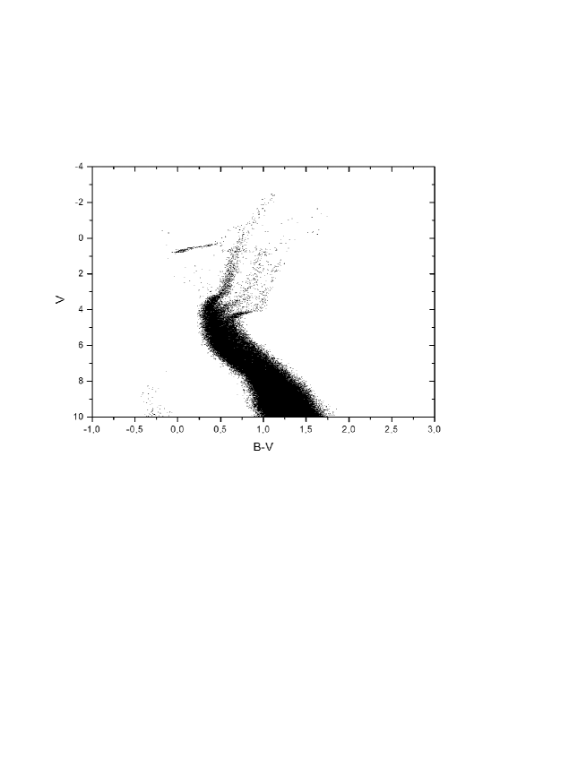
Figure 2: Same as in Fig. 1 for $f_{2}=2\times 10^{8}$ sm³g^-1s^-1.

By varying the free parameters of the model, such as the time for transition to the standard IMF, star formation efficiencies in the first ($f_{1}$) and second ($f_{2}$) episodes, the time when the matter from supernovae explosions begins to leave the system, and the fraction of lost matter, one can obtain even more complex color-magnitude diagrams in this scenario. An example is shown in Fig. 2, which corresponds to SFE on the second stage an order of magnitude higher than before ($f_{2}=2\cdot 10^{8}$ sm³g^-1s^-1), with all other parameters fixed. We stress that the transition from the diagram with two turnoff points to the one with three turnoff points is reached in this case by increasing only one parameter  — $f_{2}$ — without necessty to regulate “by hands” the sequence of several star formation bursts. In turn, the SFE may be determined by a number of factors, which at present cannot be estimated confidently. For instance, in a model in which the star formation is self-regulated by ionizing stellar radiation [21], the coefficient $f_{2}$ may be critically determined by inhomogeneity of the interstellar gas after the first burst of star formation and the fraction of ionizing radiation able to escape the proto-cluster.

An increase in the SFE results in a higher than in the latter case number of stars in the left side of the diagram. On the other hand, it leads to a faster depletion of gas, and therefore to a higher enrichment in metals ($[Z]\sim-0.3$). A fraction of the stellar population born during the period when the metallicity of the system is maximum reaches currently the extreme right of the subgiant branch. Later on, the gas metallicity decreases due to mass loss of evolved low- and intermediate-mass stars, and attains a constant level, corresponding to the one of stars currently located in the middle subgiant branch.

In the case considered here the presence of several turnoff points is a consequence of natural evolution of the stellar system, and does not require stronger assumptions about the nature of the star formation, or the existence of a stellar population with unusually high helium abundance ($Y\sim\leavevmode\nobreak\ 0.4$ [37, 38, 39, 40]), which would require an increase in the metal abundance by $\Delta Z\sim\Delta Y/5\sim 0.08$. The diagrams in Figs. 1 and  2 are plotted with accounting the observational errors. We used an approximation of the data from [41] to calculate the magnitude dependence of the rms errors.

The presence of several turnoff points indicates also that the main sequence itself has a complex structure. However, it is difficult to distinguish this structure from such kind of color-magnitude diagrams, mainly because of large observational errors for low-mass stars. In order to analyze the main sequence, we calculated several color distributions of stars along the “cuts” corresponding to a fixed value of V as suggested in [10]. Figures 3 and  4 show the dependences of the relative numbers of stars for three values of $V$. Figure 3 corresponds to the color-magnitude diagram shown in Fig. 1 and Fig. 4 to the diagram shown in Fig. 2. In these figures left panels show the distributions accounting the Gaussian smearing described above; for comparison, we show in the right panels the distributions obtained for the same model without contribution from observational errors. These figures show that even though the system does possess several main sequences, the distinction between them will not always be revealed in the observational color-magnitude diagrams.

A group of stars located on the continuing of the main sequence to $V\sim 1$, in the region occupied by so-called blue stragglers, is clearly seen. In our models, these are the youngest stars, born in late stages of evolution of the GC. For instance, the group of stars in Fig. 2 that can be identified with blue stragglers is characterized by lower metallicities ($[Z]\sim-1$) than the stars located in the right side of the diagram ($[Z]\sim-0.3$). This relatively small group of blue stragglers is born in the model shown in Fig. 2 at late evolutionary stages of stellar system when the metallicity of the gas begins to decline due to mass loss by low-mass stars with lower metallicities. Since the gas mass remained in the system by this time is small, the mass income with lower metal abundances becomes sufficient to significantly decrease the gas metallicity [6]. This identification is not acceptable in reality, however, since blue stragglers typically have anomalous chemical composition, which probably indicate their connection to active mass exchange in binaries. Note that there are no stars in the region of the blue stragglers in the color-magnitude diagrams if the model assumes that star formation does not occur at ages exceeding 1 Gyr.

3.1 A Model with Pre-Enrichment

Models with self-enrichment assume a longer evolution of the system than models with pre-enrichment. Indeed, models with pre-enrichment suggest that the bulk of metals has been already injected into the gas by some external sources on the proto-cluster stage. Therefore, over the entire subsequent cluster evolution only a slight enrichment is allowed, which does not significantly exceed the amount of the pre-enrichment. In turn, this means that in models with self-enrichment star formation has to occur in a mode that prevents the birth of stars from newly enriched matter. In other words, in such models, newly enriched matter must be swept out of the cluster before it will be able to cool radiatively and give rise to new generations of stars. A sufficient condition for such a mode to occur is a rapid star formation on early stages, which results after several Myr in a large energy release enough to prevent the enriched gas from cooling. A rough estimate of this condition can be obtained by assuming that the supernovae energy rate exceeds the total rate of radiation losses in the gas:

$$\nu_{sn}E_{sn}>\Lambda(T)n^{2}V,$$ (12)

where $\nu_{sn}$ and $E_{sn}=10^{51}$ erg are the supernova rate in a GC, and the supernova explosion energy, $\Lambda(T)\sim 3\cdot 10^{-23}$ erg sm³s^-1 is the rate of radiative losses at gas temperatures behind the shock $T\sim(1-3)\cdot 10^{5}$ K, $n$ is the number density of the gas and $V$ is the volume of a GC. For $n\sim 10^{3}$  ^-3 and $R\sim 20$ pc, the estimate (12) gives $\nu_{sn}\sim 3$ supernovae per year, which is equivalent to a SFE $f\sim 2\cdot 10^{8}$ sm³g^-1s^-1 an order of magnitude higher than commonly assumed value. This is obviously an overestimate, since the binding energy of globular clusters is low, and a substantially lower energy release is sufficient to remove the gas from the cluster. Indeed, it is easy to show that, even for the SFE assumed above, $f\sim 2\cdot 10^{7}$ sm³g^-1s^-1, the number of supernovae that would explode in the cluster over time sufficient for the volume filling factor of the hot gas to equal one is $N_{sn}\sim 600$, whose total energy release exceeds the binding energy of a cluster with mass $M=10^{6}M_{\odot}$ and initial radius $R=20$ pc by two orders of magnitude. Below we will adopt precisely this SFR for the model with pre-enrichment, $f=2\cdot 10^{7}$ sm³g^-1s^-1.

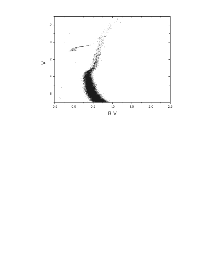
Figure 5: Color-magnitude diagram for the model with primordial self-enrichment $[Z]_{\rm in}=-1.5$; the SFR is specified to be zero at $t=10^{8}$ yr.

Figure 5 shows the results of computing the color-magnitude diagram for a GC with a mass of $M=10^{6}M_{\odot}$ which is pre-enriched to metallicity $[Z]=-1.5$ and begins its evolution with radius $R=20$ pc and the SFE given above. Similar to the previous figures, Fig. 5 is plotted with accounting a Gaussian smearing. An important feature of this model is that, when the first supernovae begin to eject heavy elements at about $t>10^{7}$  yr, the bulk of the matter with the initial chemical abundances is already contained in stars. Thus if we assume that under these circumstances the gas ejected by supernovae is easily removed from the system, the number of stars with metallicities exceeding the initial value will be negligibly small. Figure 5 shows the results for a model GC in which practically all stars have the initial metallicity.

It is obvious that a similar diagram can also be obtained in a model with self-enrichment if the parameters of star formation are such that the separation (in $B-V$) between the main sequences is smaller than the observational errors. In this case, it is practically impossible to distinguish between the two populations on observational color-magnitude diagrams. As an illustration of this situation, Figures 6 and 7 present a color-magnitude diagram and color distributions of relative numbers of stars, respectively. In this model, the first burst of star formation has $M_{min}=8M_{\odot}$, $M_{max}=100M_{\odot}$, and $f_{1}=2.6\cdot 10^{5}$ sm³g^-1s^-1; the transition to the second burst with a “standard” IMF occurs at $t=10$ Myr; the second burst of star formation has $M_{min}=8M_{\odot}$, $M_{max}=100M_{\odot}$, and $f_{2}=2\cdot 10^{7}$ sm³g^-1s^-1, with 99.7% of the matter ejected by supernovae swept out of the cluster after $t=10$ Myr. In this case, the absence of multiple turnoff points is a consequence of a larger fraction mass loss than in the model shown in Fig. 1. Note that the model computation produces two stellar populations which correspond to low metallicities $[Z]=-2$ and -1.6; this makes it even more difficult to distinguish between the populations, due to the proximity of the isochrones for low metallicities.

Thus, the absence of multiple turnoff points in observational color-magnitude diagram does not necessarily mean that matter of the corresponding GC was pre-enriched in heavy elements, since the separation that arises in models with self-enrichment may be smaller than the errors in the colors. In self-enrichment scenarios, it may be easier to distinguish stars with different metallicities within more massive GCs. In fact, we would expect a decrease of the metallicity of the main fraction of stars with increasing cluster mass [4, 6]. At the same time the later generation of stars has as a rule metallicities close to the asymptotic value $[Z]\sim-0.8$, which only weakly depends on the cluster mass. Observing this separation for GCs with masses of $M\sim 10^{5}\leavevmode\nobreak\ M_{\odot}$ requires an increased accuracy for magnitudes of $\Delta m\sim 0.03-0.07$. The proposed interpretation of the color-magnitude diagram of $\omega$ Cen as having multiple main sequence turnoff points with several distinct stellar populations is justified by spectroscopic measurements of metallicities in $\omega$ Cen. Several main sequences are also observed in NGC 2808 [43]. With accounting the fact that spectroscopic metallicities of different branches of the main sequence in NGC 2808 are nearly equal, Piotto et al. [42] suggest a scenario where the multiplicity of the main sequence is connected with different helium abundances ($Y\sim 0.24-0.4$). Thus, the two cases — $\omega$ Cen and NGC 2808 — seem to represent two possible scenarios for the evolution of GCs: one produces several populations with different metallicities, while another produces populations with similar metallicities but very different helium abundances. From this point of view in order to clarify the origin of this multiplicity, detection of multiple main sequence turnoff points in other Galactic GCs and a precise spectroscopic determinations of the iron abundance will play crucial role.

4 CONCLUSIONS

We have applied a simple single-zone model to analyze color-magnitude diagrams for globular clusters. Our results show the following.

1. The presence of two or more main sequence turnoff points in the color-magnitude diagrams of GCs can be naturally explained in models with self-enrichment, with an initial stellar mass function that is initially shifted toward high masses, but then changes to a normal IMF.

2. This represents an argument in favor of the self-enrichment of GCs with multiple turnoffs (such as $\omega$ Cen) in metals due to internal processes within the GC.

3. On the other hand, the uncertainties in the luminosities and magnitudes of stars in GCs are still fairly large, and do not always enable resolution of the main sequences in color-magnitude diagrams into subgroups. In other words, the absence of multiple turnoff points does not necessarily require an external (pre-) enrichment in metals.

5 ASKNOWLEDGMENTS

The authors thank V. I. Korchagin for discussions. This study was supported by the Russian Foundation for Basic Research (project code 06-02-16819) and the State Education Agency (project code RNP 2.1.1.3483).

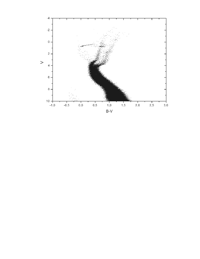
Figure 1: Color-magnitude diagram for bimodal star formation. The initial star formation episode has $M_{min}=8\leavevmode\nobreak\ M_{\odot}$ and $f_{1}=2.6\times 10^{5}$ sm³g${-1}$s^-1, and lasts for $10^{7}$ yr; the second star formation episode has $M_{min}=0.1\leavevmode\nobreak\ M_{\odot}$ and $f_{2}=2\times 10^{7}$ sm³g^-1s^-1. At $t=10^{7}$ yr, 95% of the matter ejected by supernovae has left the cluster.

Figure 3: Number of stars as a function of the color corresponding to cuts of the color-magnitude diagram shown in Fig. 1 for $V=5,\leavevmode\nobreak\ 6,\leavevmode\nobreak\ 7$. Diagrams (a), (b), (c) correspond to the plotted histogram, taking into account the observational errors, while diagrams (d), (e), (f) correspond to the plotted histogram without accounting observational errors.

Figure 4: Same as in Fig. 3 for analogous cuts of the color-magnitude diagram presented in Fig. 2.

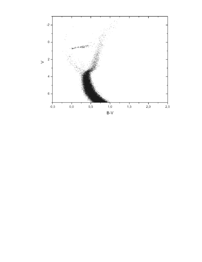
Figure 6: Same as in Fig. 1, but with the fraction of matter ejected by supernovae and lost by the system at time $t=10^{7}$ yr being 99.7%.

Figure 7: Same as in Fig. 3 for the analogous cuts of the color-magnitude diagram presented in Fig. 7.

References

- [1] W.E.Harris andR. E.Pudritz,Astrophys. J. 429, 177 (1994).
- [2] Marsakov V. A. and Suchkov A. A., Sov. Astron. Lett. 2, 148 (1976).
- [3] J. P. Brodie and J. Strader, Ann. Rev. Astron. Astrophys. 44, 193 (2006).
- [4] G. Parmentier and G. Gilmor, Astron. Astrophys. 378, 97 (2001).
- [5] G. Parmentier, E. Jehin, P. Magain, et al., Astron. Astrophys. 352, 138 (1999).
- [6] M. V. Kas yanova and Yu. A. Shchekinov, Astron. Rep. 49, 863 (2005).
- [7] M. H Hénon, Ann. d Astrophys. 24, 369 (1961).
- [8] L. Spitzer and J. M. Shull, Astrophys. J. 201, 773 (1975).
- [9] V. G. Surdin, Sov. Astron. 23, 648 (1979).
- [10] S. Villanova, G. Piotto, I. R. King, et al., Astrophys. J. 663, 296 (2007).
- [11] F. D Antona, M. Bellazzini,V. Caloi, et al., Astrophys. J. 631, 868 (2005).
- [12] T. Tsujimoto and T. Shigeyama, Astrophys. J. 590, 803 (2003).
- [13] N. B. Suntzeff and R. P. Kraft, Astron. J. 111, 1913 (1996).
- [14] O. Y. Gnedin,H. Zhao, J. E. Pringle, et al., Astrophys. J. 568, L23 (2002).
- [15] F. Matteucci and L. Greggio, Astron. Astrophys. 154, 279 (1989).
- [16] C. Firmani and A. V. Tutukov, Astron. Astrophys. 264, 37 (1992).
- [17] B. M. Shustov, D. S. Wiebe, and A. V. Tutukov, Astron. Astrophys. 317, 397 (1997).
- [18] C. Chiappini, F. Matteucci, and R. Gratton, Astrophys. J. 477, 765 (1997).
- [19] D. S. Wiebe, A. V. Tutukov, and B. M. Shustov, Astron. Rep. 42, 1 (1998).
- [20] M. Schmidt, Astrophys. J. 129, 243 (1959).
- [21] D. P. Cox, Astrophys. J. 265, L61 (1983).
- [22] E. E. Salpeter, Astrophys. J. 121, 161 (1955).
- [23] S. E.Woosley and T. A.Weaver, Astrophys. J., Suppl. Ser. 101, 181 (1995).
- [24] K. Nomoto, M. Hashimoto, T. Tsujimoto, and F.- K. Thielemman, Nucl. Phys. A. 616, 79c (1997).
- [25] L. Greggio and A. Renzini, Astron. Astrophys. 118, 217 (1983).
- [26] L. Girardi, A. Bressan, C. Chiosi, et al., Astron. Astrophys., Suppl. Ser. 117, 113 (1996).
- [27] F. Fagotto, A. Bressan, G. Bertelli, and C. Chiosi, Astron. Astrophys., Suppl. Ser. 104, 365 (1994).
- [28] F. Fagotto, A. Bressan, G. Bertelli, and C. Chiosi, Astron. Astrophys., Suppl. Ser. 105, 29 (1994).
- [29] F. Fagotto, A. Bressan, G. Bertelli, and C. Chiosi, Astron. Astrophys., Suppl. Ser. 105, 39 (1994).
- [30] F. Fagotto, A. Bressan, G. Bertelli, and C. Chiosi, Astron. Astrophys., Suppl. Ser. 100, 647 (1993).
- [31] D. Vandenbergh, F. Harteick, and P. Dawson, Astrophys. J. 266, 747 (1983).
- [32] T. Lejeune, F. Cuisiner, and R. Buser, Astron. Astrophys., Suppl. Ser. 125, 229 (1997).
- [33] T. Lejeune, F. Cuisiner, and R. Buser, Astron. Astrophys., Suppl. Ser. 130, 65 (1998).
- [34] R. E. S. Clegg and D. Middlemass, Mon. Not. R. Astron. Soc. 228, 759 (1987).
- [35] G. A. Bruzual, in Galaxies at High Redshift, Ed. by I. Perez-Fournon, M. Balcells, F.Moreno-Insertis, and F. Sanchez (Cambridge Univ. Press, Cambridge, 2003), p. 185.
- [36] N. Yoshida, K. Omukai, L. Hernquist, and T. Abel, Astrophys. J. 652, 6 (2006).
- [37] L. R. Bedin and G. Piotto, Astrophys. J. 605, 125 (2004).
- [38] J. E. Norris, Astrophys. J. 612, 25 (2004).
- [39] G. Piotto, S. Villanova, L. R. Bedin, et al., Astrophys. J. 621, 777 (2005).
- [40] Y.W. Lee, et. al. Astrophys. J. 621, 57 (2005).
- [41] Padova Globular Cluster Group, http://dipastro. pd.astro.it/globulars.
- [42] G. Piotto, L. R. Bedin, J. Anderson, et al., Astrophys. J. 661, L53 (2007).