HD-THEP-08-18 Unifying cosmological and recent time variations of fundamental couplings

Abstract

A number of positive and null results on the time variation of fundamental constants have been reported. It is difficult to judge whether or not these claims are mutually consistent, since the observable quantities depend on several parameters, namely the coupling strengths and masses of particles. The evolution of these coupling-parameters over cosmological history is also a priori unknown. A direct comparison requires a relation between the couplings. We explore several distinct scenarios based on unification of gauge couplings, providing a representative (though not exhaustive) sample of such relations. For each scenario we obtain a characteristic time dependence and discuss whether a monotonic time evolution is allowed. For all scenarios, some contradictions between different observations appear. We show how a clear observational determination of non-zero variations would test the dominant mechanism of varying couplings within unified theories.

1 Introduction

Any observation of a time variation of “fundamental constants” would be a far-reaching discovery. There are various claims for a detection, and many more observations indicating a null variation: criteria for judging their mutual consistency would be useful. We investigate whether a simple scenario exists which can account for several observational claims simultaneously and is consistent with unification of Standard Model (SM) gauge couplings. Several observations motivate such a study. First, the claimed deviations from the present value of the fine structure constant $\alpha$, or the proton-to-electron mass ratio $\mu$, observed in quasar absorption systems. Second, the discrepancy between the primordial ⁷Li abundance expected from standard nucleosynthesis (BBN) and seen in old halo stars, which may be explained by a variation of “constants” within a unified framework [1, 2]. Third, the theoretical insight that scalar fields cannot be exactly constant over the entire cosmological evolution, and that a possible “late” time evolution can play an important role in the dynamics of the expanding Universe. A time variation of couplings arising from the evolution of a “cosmon” field in so-called “quintessence scenarios” [3, 4] would link these variations to observables in cosmology [5, 6].

Due to the many unknowns of the underlying particle physics models and the partly contradictory present observational situation, a systematic treatment is not easy, and may even seem premature. Nevertheless we consider a first attempt to be useful, in order to discuss strategies that can be used to compare variations of different observables. The power of the proposed method will only become clear if and when future observations present a less ambiguous picture.

The basic approach in the present paper relates the fractional variations of different fundamental couplings $G_{k}$, such as the fine structure constant $\alpha$, the proton-electron mass ratio $\mu$ or the ratio of the nucleon mass to the Planck mass, by an assumption of proportionality, with fixed “unification coefficients” $d_{k}$. The choice of the values of $d_{k}$ is in turn determined within different scenarios of varying parameters in unified theories (GUTs) where the gauge couplings of the Standard Model converge at a unification scale $M_{X}$. The assumption of time-independent coefficients $d_{k}$ covers a large class of possible models for varying couplings. This assumption is, however, not a necessity, and we will describe specific quintessence models where it may not be realized in a forthcoming paper [7].

In Section 2 of this paper we review observational determinations of the variation or constancy of couplings, considering five types of methods: early-universe cosmology, astrophysical spectroscopy, nuclear physics in the Earth and the Solar System, gravitational physics, and atomic clock comparisons. In Section 3 we introduce the unification of couplings (Grand Unified Theory, GUT) and determine the implications of unification and supersymmetry (SUSY) for the Standard Model parameters and for the observables we consider. We further define six unified scenarios by considering different possibilities for the variation of the Fermi scale and the superpartner masses. Within each scenario we reduce the various observational results to constraints on the time evolution of a single fundamental coupling, and discuss the mutual consistency of observations.

In Section 4 six cosmological epochs are introduced, and the constraints on variation deduced in Section 3 are collected into a set of “evolution factors” for each unified scenario. These evolution factors are a measure of the overall size of coupling evolution between a given epoch and the present. We then determine for each scenario to what extent a monotonic variation over time can be consistent with the data. Section 5 draws some general conclusions.

In a subsequent paper [7] we will investigate the scalar field dynamics that could give rise to a small but nonzero variation of couplings. The presence of a cosmologically varying degree of freedom gives rise to important additional effects. It affects gravity on large scales, altering the expansion of the Universe and potentially giving rise to the observed late-time acceleration. Also on local scales, a light field weakly coupled to matter produces long-range forces which are tightly constrained [8] by Solar System precision tests of gravity and the null results of experiments testing the Weak Equivalence Principle. Combining all these considerations leads to tighter constraints on models but also offers more possibilities to test them.

2 Data: variations and constraints

Here we review and discuss the observational data that we will consider in our effort to obtain a unified picture of time variation of couplings. We summarize the results that are most relevant for our analysis in Table 1.

Method	redshift	$\Delta\ln\alpha$	$\Delta\ln\mu$	$\Delta\ln Gm_{N}^{2}$	$\Delta\ln x$	$\Delta\ln y$	$\Delta\ln F$	$\Delta\ln F^{\prime}$	$\Delta\ln\lambda_{187}$
		$[10^{-6}]$	$[10^{-5}]$	$[10^{-2}]$	$[10^{-5}]$	$[10^{-5}]$	$[10^{-5}]$	$[10^{-4}]$	$[10^{-2}]$
Oklo $\alpha$ [45]	0.14	$0.00\pm 0.06$
21cm [41]	0.247					$-0.20\pm 0.44$
Sun [57]	0.43			$0\pm 0.72$
Heavy/HI, low-z [42]	0.40				$1.0\pm 1.7$
Meteorite [49]	0.44								$3.3\pm 3.2$
M$\alpha$ epoch 2 [28]	0.65	$-2.9\pm 3.1$
Ammonia [39]	0.68		$0.06\pm 0.19$
21cm [41]	0.685					$-0.16\pm 0.54$
HI / OH [43]	0.765						$0.4\pm 1.1$
Absorption [31]	1.15	$-0.1\pm 1.8$
$M\alpha$ epoch 3 [28]	1.47	$-5.8\pm 1.3$
Absorption [32]	1.84	$5.7\pm 2.7$
Heavy/HI, high-z [42]	2.03				$0.6\pm 1.9$
$H_{2}$ [37]	2.59		$2.78\pm 0.88$
$M\alpha$ epoch 4 [28]	2.84	$-8.7\pm 3.7$
$H_{2}$ [37]	3.02		$2.06\pm 0.79$
Neutron stars [60]	3.3			$-0.7\pm 2.4$
CII / CO [44]	4.69							$1.4\pm 1.5$
CII / CO [44]	6.42							$0.1\pm 1.0$
CMB [24], [26]	$10^{3}$	$0^{+1\times 10^{4}}_{-3\times 10^{4}}$		$0^{+7}_{-6}$

Table 1: Observational $1\sigma$ bounds on variations. Observables are defined as $\mu\equiv m_{p}/m_{e}$, $x\equiv\alpha^{2}g_{p}\mu^{-1}$, $y\equiv\alpha^{2}g_{p}$, $F\equiv g_{p}[\alpha^{2}\mu]^{1.57}$, $F^{\prime}\equiv\alpha^{2}/\mu$. The given redshift may denote a single measurement, or an averaged value over a certain range: see main text. The two CMB bounds are independent of each other. Our BBN bounds cannot be displayed in this form.

2.1 Early universe: BBN and CMB

The earliest processes for which Standard Model physics can be tested are BBN ($z\sim 10^{10}$) and CMB ($z\sim 10^{3}$). Hence they constitute the most far-reaching tests of a possible variation of couplings.

BBN

The influence of varying constants on BBN has been studied extensively [2, 9, 10, 11, 12, 13, 14, 15, 16, 17, 18, 19] (see also [20] and references therein). The method developed in [1, 12] accounts for possible simultaneous variations of different fundamental parameters, while previous studies restricted attention to the variation along one particular direction in parameter space.

Our approach in [1] was first to calculate the leading dependence of BBN abundances on a set of “nuclear parameters”, comprising elementary particle coupling strengths and masses and nuclear binding energies. In a second step, these nuclear parameters were related to fundamental parameters in particle theory, which allowed us to consider (at linear order) any combination of variations at BBN. Thus, our results are independent of any assumptions about unification.

In an extension of our previous treatment, we include in Appendix A the possible effect of varying constants at CMB on the input parameter $\eta$ of our BBN procedure. The important parameter is here the variation of $m_{N}/M_{\rm P}$ at CMB relative to the variation at BBN, where $m_{N}$ is the nucleon mass and $M_{\rm P}$ is the “reduced” Planck mass. We consider two limiting cases. First, when $\Delta(m_{N}/M_{\rm P})_{|\rm CMB}\ll\Delta(m_{N}/M_{\rm P})_{|\rm BBN}$: then our previous results hold. In the second case, with $\Delta(m_{N}/M_{\rm P})_{|\rm CMB}\simeq\Delta(m_{N}/M_{\rm P})_{|\rm BBN}$, the value of $\eta$ may be significantly rescaled.

Our result for the leading dependence of primordial abundances $Y_{a}$ on fundamental particle physics parameters $G_{k}=(G,\alpha,\langle\phi\rangle,m_{e},\delta_{q},\hat{m})$ is summarized in Table 2. Here $\delta_{q}\equiv m_{d}-m_{u}$ denotes the light quark mass difference, $\hat{m}\equiv(m_{d}+m_{u})/2$ the average light quark mass, and $\langle\phi\rangle$ is the expectation value of the Higgs scalar that determines the Fermi scale of the weak interactions. The variation of dimensionful quantities is defined relative to the QCD strong coupling scale $\Lambda_{c}$. We found that only D, ⁴He and ⁷Li can be used to constrain parameters at BBN. Whilst Table 2 only gives linear dependencies, we can account for nonlinearities by running the full BBN code with the appropriate variations [1].

$\partial\ln Y_{a}/\partial\ln G_{k}$	D	4He	7Li
$G$	0.94	0.36	-0.72
$\alpha$	3.6	1.9	-11
$\langle\phi\rangle$	1.6	2.9	1.7
$m_{e}$	0.46	0.40	-0.17
$\delta_{q}$	-2.9	-5.1	-2.9
$\hat{m}$	17	-2.7	-61
$\eta$	-1.6	0.04	2.1

Table 2: Sensitivity of abundances $Y_{i}$ to variations of fundamental parameters $G_{k}$ and the baryon-to-photon ratio $\eta$.

The current observational and theoretical values for the $Y_{a}$ are given in Table 3, where $Y_{p}$ is the helium mass fraction equal to four times the ratio of ⁴He number density to hydrogen.

Abundance	Observational	Theoretical
D/H	$(2.8\pm 0.4)\times 10^{-5}$	$(2.61\pm 0.04)\times 10^{-5}$
$Y_{p}$	$0.249\pm 0.009$	$0.2478\pm 0.0002$
7Li/ H	$(1.5\pm 0.5)\times 10^{-10}$	$(4.5\pm 0.4)\times 10^{-10}$

Table 3: Current observational and theoretical primordial abundances

The uncertainty in the $\eta$ determination, $\eta=(6.20\pm 0.16)\times 10^{-10}$ (WMAP5 plus BAO and SN, [21]) yields a further correlated error for the abundances, which can be treated using the method of [22]. For any given set of fundamental variations we can define

$$\chi^{2}\equiv\sum_{i,j}(Y_{i}-Y_{i}^{obs})w_{ij}(Y_{j}-Y_{j}^{obs}),$$ (1)

with the inverse weight matrix

$$w_{ij}=\left[\sigma^{2,\eta}_{ij}+\delta_{ij}(\sigma^{2}_{obs,i}+\sigma^{2}_{th,i})\right]^{-1},$$ (2)

where

$$\sigma^{2,\eta}_{ij}\equiv Y_{i}Y_{j}\frac{\partial\ln Y_{i}}{\partial\ln\eta}\frac{\partial\ln Y_{j}}{\partial\ln\eta}\left(\frac{\Delta\eta}{\eta}\right)^{2}.$$ (3)

We take, as in [1],

$$\frac{\partial\ln({\rm D/H},Y_{\rm p},\mbox{${{}^{7}}$Li/H})}{\partial\ln\eta}=(-1.6,\ 0.04,\ 2.1).$$ (4)

The $1(2)\sigma$ error contour is given by $\chi^{2}/\nu\leq 1(4)$ where $\nu$ is the number of degrees of freedom. As the final abundances depend on variations of all fundamental constants, we have to evaluate the variations allowed by BBN for every model separately.

It has been pointed out that the important ⁸Be resonance very near the ground states of ⁷Be$+n$ and ⁷Li$+p$ makes the exchange reaction converting ⁷Be into ⁷Li potentially sensitive to variations in nuclear forces. We give an estimate of this sensitivity in Appendix B and show that it is unlikely to be significant for the range of variations that we consider.

In the light of complex astrophysics which may affect the extraction of the primordial ⁷Li fraction [23], we also consider bounding the variations using deuterium and ⁴He alone. This yields a value consistent with zero for variations at BBN, since these abundances are consistent with standard BBN.

CMB

In principle, $\alpha$ and $G$ are bounded by CMB, but there are significant degeneracies with other cosmological parameters [24, 25]: see also the discussion in Appendix A. Current bounds are

$$0.95<\frac{\alpha_{\rm CMB}}{\alpha_{0}}<1.02\qquad(2\sigma).$$ (5)

The CMB anisotropies may also be used to constrain the variation of Newton’s constant $G$. The resulting bound depends on the form of the variation of $G$ from the time of CMB decoupling to now. Using a step function one finds [26, 27]

$$0.95\leq\frac{G}{G_{0}}\leq 1.05\qquad(2\sigma),$$ (6)

where the instantaneous change in $G$ may happen at any time between now and CMB decoupling. Using instead a linear function of the scale factor $a$, the bound is

$$0.89\leq\frac{G}{G_{0}}\leq 1.13\qquad(2\sigma).$$ (7)

Note that here, as in most studies of time-dependent $G$, units are implicitly defined such that the elementary particle masses (and thus the mass of gravitating bodies, if gravitational self-energy is neglected) are constant. The relevant bound on dimensionless parameters concerns $Gm_{N}^{2}\equiv(m_{N}/M_{\rm P})^{2}(8\pi)^{-1}$.

2.2 Quasar absorption spectra

The observation of absorption spectra of distant interstellar clouds allows to probe atomic physics over large time scales. Comparing observed spectra with the spectra observed in the laboratory gives bounds on the possible variation of couplings. Different kinds of spectra (atomic, molecular, …) are sensitive to different parameters, principally $\alpha$ and $\mu\equiv m_{p}/m_{e}$.

Atomic spectra are primarily sensitive to $\alpha$. Several groups using various methods of modelling and numerical analysis have published results; we quote here only the latest bounds. Murphy and collaborators [28] studied the spectra of 143 quasar absorption systems over the redshift range $0.2<z_{abs}<4.2$. Their most robust estimate is a weighted mean

$$\frac{\Delta\alpha}{\alpha}=(-0.57\pm 0.11)\times 10^{-5}.$$ (8)

In discussing unified models in Section 4, we will define various “epochs” for the purpose of collating data and comparing them with models over certain ranges of redshift. The 143 data points are then assigned to different epochs: we choose to put boundaries at $z=0.81$ and $z=2.4$, thus we obtain three sub-samples

$$z <0.81, N_{sys} =18, \langle z\rangle =0.65, \frac{\Delta\alpha}{\alpha} =(-0.29\pm 0.31)\times 10^{-5}$$

$$0.81<z <2.4 N_{sys} =85, \langle z\rangle =1.47, \frac{\Delta\alpha}{\alpha} =(-0.58\pm 0.13)\times 10^{-5}$$

$$z >2.4, N_{sys} =40, \langle z\rangle =2.84, \frac{\Delta\alpha}{\alpha} =(-0.87\pm 0.37)\times 10^{-5}.$$ (9)

Here we have used the “fiducial sample” of [29], the weighted average has been taken, and we have included [30] the 15 additional samples used in [28]. For convenience we will refer to these results as “M$\alpha$”.

Further results have been obtained by Levshakov et al. [32], and reported in [31]:

$$\frac{\Delta\alpha}{\alpha} =(-0.01\pm 0.18)\times 10^{-5}, z_{abs} =1.15$$

$$\frac{\Delta\alpha}{\alpha} =(0.57\pm 0.27)\times 10^{-5}, z_{abs} =1.84.$$ (10)

Previously [33, 34] more stringent null results were claimed, but doubts have been cast [35] (see also [36]) on the validity of the statistical analysis. We note that the value for $z=1.84$ has an opposite sign of variation to the M$\alpha$ result, though the variation does not have high statistical significance. The observational situation is clearly unsatisfactory.

Vibro-rotational transitions of molecular hydrogen $H_{2}$ are sensitive to $\mu\equiv m_{p}/m_{e}$. From H₂ lines of two quasar absorption systems (at $z=2.59$ and $z=3.02$) a variation is found [37] of

$$\frac{\Delta\mu}{\mu}=(2.4\pm 0.6)\times 10^{-5},$$ (11)

taking a weighted average. We will refer to this result as “R$\mu$” after Reinhold et al. The individual systems yield [37]

$$\frac{\Delta\mu}{\mu} =(2.78\pm 0.88)\times 10^{-5}, z_{abs} =2.59$$

$$\frac{\Delta\mu}{\mu} =(2.06\pm 0.79)\times 10^{-5}, z_{abs} =3.02.$$ (12)

Recently the $z=3.02$ system has been reanalyzed [38], with the result that the claimed significance of Eq. (2.2) was not reproduced, and the absolute magnitude of the variation is bounded by $|\Delta\mu/\mu|\leq 4.9\times 10^{-5}$ at $2\sigma$, or

$$|\Delta\mu/\mu|\leq 2.5\times 10^{-5},\qquad z_{abs}=3.02\quad(1\sigma).$$ (13)

The inversion spectrum of ammonia has been used to bound $\mu$ precisely at lower redshift [39]. Recently the single known NH₃ absorber system at cosmological redshift has been analysed [40], yielding

$$\frac{\Delta\mu}{\mu}=(0.74\pm 0.89)\times 10^{-6},\qquad z=0.68.$$ (14)

This is a considerably stricter bound but applies at a different epoch. Extrapolation to today with linear time dependence gives $\dot{\mu}/\mu=(1.2\pm 1.4)\times 10^{-16}\,$y^-1.

The 21cm HI line and molecular rotation spectra are sensitive to $y\equiv\alpha^{2}g_{p}$, where $g_{p}$ is the proton g-factor. Bounds on this quantity from [41] are

$$\frac{\Delta y}{y} =(-0.20\pm 0.44)\times 10^{-5}, z =0.247$$

$$\frac{\Delta y}{y} =(-0.16\pm 0.54)\times 10^{-5}, z =0.685.$$ (15)

Further, the comparison of UV heavy element transitions with HI line probes for variations of $x\equiv\alpha^{2}g_{p}\mu^{-1}$ [42]: the weighted mean of nine analysed systems yields

$$\frac{\Delta x}{x}=(0.63\pm 0.99)\times 10^{-5},\quad 0.23<z_{abs}<2.35.$$ (16)

However, we note that i) the systems lie in two widely-separated low-redshift ($0.23<z<0.53$) and high-redshift ($1.7<z<2.35$) ranges; and ii) these two sub-samples have completely different scatter, $\chi^{2}/\nu$ about the mean for the low- and high-redshift systems being $0.33$, and $2.1$, respectively. Hence we consider two samples, with average redshift $z=0.40$ (5 systems) and $z=2.03$ (4 systems). With expanded error bars in the high-redshift sample (after “method 3” of [42]) we find

$$\frac{\Delta x}{x} =(1.02\pm 1.68)\times 10^{-5}, \langle z\rangle =0.40$$

$$\frac{\Delta x}{x} =(0.58\pm 1.94)\times 10^{-5}, \langle z\rangle =2.03.$$ (17)

The comparison of HI and OH lines is sensitive to changes in $F\equiv g_{p}\left[\alpha^{2}\mu\right]^{1.57}$ [43] and yields

$$\frac{\Delta F}{F}=(0.44\pm 0.36^{stat}\pm 1.0^{sys})\times 10^{-5},\quad z=0.765.$$ (18)

A similar method comparing CII and CO lines has very recently been proposed at high redshift [44] yielding the best bound at redshifts $>4.5$. The following bounds on $F^{\prime}\equiv\alpha^{2}/\mu$ are obtained for two systems:

$$\frac{\Delta F^{\prime}}{F^{\prime}} =(0.1\pm 1.0)\times 10^{-4}, z =6.42$$

$$\frac{\Delta F^{\prime}}{F^{\prime}} =(1.4\pm 1.5)\times 10^{-4}, z =4.69.$$ (19)

2.3 Terrestrial and Solar System nuclear constraints

Oklo natural reactor

From modelling nuclear reaction processes which happened in the Oklo mine about two billion years ago ($\Delta t\simeq 1.8\times 10^{9}\,$y, $z\sim 0.14$ with WMAP5 best fit cosmology) one can in principle bound the variation of $\alpha$ over this period. The determination of $\Delta\ln\alpha$ at the time of the reactions results from considering the possible shift, due to variation of electromagnetic self-energy, in the position of a very low-lying neutron capture resonance of ¹⁴⁹Sm. The analysis of [45] gives the bound (taken as 1$\sigma$)

$$-5.6\times 10^{-8}<\Delta\alpha/\alpha<6.6\times 10^{-8}.$$ (20)

For a linear time dependence this results in the bound

$$|\dot{\alpha}/\alpha|\leq 3\times 10^{-17}{\rm y}^{-1}.$$

A more recent analysis using different reactor models and consequently different neutron spectra [46] found

$$-2.4\times 10^{-8}\leq\Delta\alpha/\alpha\leq 1.1\times 10^{-8}$$

with an additional nonzero solution (due to the other branch of the resonance peak) at $\Delta\alpha/\alpha\simeq 8\times 10^{-8}$. We will consider the more conservative bound.

Note that these results concern varying $\alpha$ only. If other parameters affecting nuclear forces, in particular light quark masses, are allowed to vary, the interpretation of this bound becomes unclear [47, 48] since it depends on a nuclear resonance of ¹⁵⁰Sm whose properties are very difficult to investigate from first principles. In the absence of a resolution to this problem we consider Oklo as applying only to the $\alpha$ variation in each model. In scenarios where several couplings vary simultaneously we do not consider strong cancellations. Nevertheless, we allow for a certain degree of accidental cancellation and therefore multiply the error on the bound Eq. (20) by a factor three.

Meteorite dating

Long-lived $\alpha$- or $\beta$-decay isotopes may be sensitive probes of cosmological variation [49, 47, 50]. Their (generally) small $Q$-values result from accidental cancellations between different contributions to nuclear binding energy, depending on fundamental couplings in different ways, thus the sensitivity of the decay rate may be enhanced by orders of magnitude.

The best bound concerns the ¹⁸⁷Re $\beta$-decay to osmium with $Q_{\beta}=2.66\,$keV. The decay rate $\lambda_{187}$ is measured at present in the laboratory, and also deduced by isotopic analysis of meteorites formed about the same time as the solar system, $t_{\rm Met}\simeq 4.6\times 10^{9}\,$y ago ($z\simeq 0.44$). More precisely, the ratio $\lambda_{187}/\lambda_{\rm U}$, averaged over the time between formation and the present, is measurable [49, 51], where $\lambda_{\rm U}$ is the rate of some other decay (for example uranium) used to calibrate meteorite ages. The experimental values of $\lambda_{187}$ imply (setting $\lambda_{U}$ to a constant value)

$$t_{\rm Met}^{-1}\int_{-t_{\rm Met}}^{0}\frac{\Delta\lambda_{187}(t)}{\lambda_{187}}\,dt=0.016\pm 0.016.$$ (21)

Since the redshift back to $t_{\rm Met}$ is relatively small, we obtain bounds on recent time variation by assuming a linear evolution up to the present, for which the LHS is $-(t_{\rm Met}/2)\dot{\lambda}_{187}/\lambda_{187}$ and the fractional rate of change is bounded by

$$\frac{\dot{\lambda}_{187}}{\lambda_{187}}\simeq(-7.2\pm 6.9)\times 10^{-12}\,{\rm y}^{-1}.$$ (22)

Projected back to $t_{\rm Met}$ this gives the bound $\Delta\ln\lambda_{187}\simeq 0.033\pm 0.032$ ($z\simeq 0.44$). This is a conservative bound unless the time variation has recently accelerated (which we consider unlikely), or there are significant oscillatory variations over time.

The decay rate varies as [47]

$$\lambda_{187}\propto G_{F}^{2}Q_{\beta}^{3}m_{e}^{2}\propto\langle\phi\rangle^{-2}Q_{\beta}^{3}y_{e}^{2}$$

where $y_{e}$ is the electron Yukawa coupling. Variation in $Q_{\beta}$ is determined by the near-cancellation between the nuclear Coulomb self-energy and asymmetry energy of ¹⁸⁷Re and ¹⁸⁷Os, and the nucleon masses, via

$$\Delta{Q_{\beta}}\simeq 0.77\Delta{a_{A}}-26\Delta{a_{C}}+\Delta(\delta_{N}-m_{e}),$$

where $a_{A}\simeq 23.7\,$MeV and $a_{C}\simeq 0.71\,$MeV are the asymmetry and Coulomb terms of the semi-empirical mass formula and $\delta_{N}\equiv m_{n}-m_{p}$ is the nucleon mass splitting. Thus the fractional variation in $\lambda_{187}$ is

$$\Delta\ln\frac{\lambda_{187}}{m_{N}}\simeq 2.1\times 10^{4}\,\Delta\ln\frac{a_{A}}{m_{N}}-2.1\times 10^{4}\,\Delta\ln\alpha+880\,\Delta\ln\frac{\delta_{N}-m_{e}}{m_{N}}.$$ (23)

Since the possible dependence of “control” decay rates $\lambda_{\rm U}/m_{N}$ on nuclear or fundamental parameters is much weaker than that of $\lambda_{187}/m_{N}$, we use this result for the variation of $\lambda_{187}$ in units where $\lambda_{\rm U}$ is constant. Then using relations derived in [52] and considering also the effect of varying $m_{s}$ on the nucleon mass,

$$\Delta\ln\frac{\delta_{N}-m_{e}}{m_{N}} \simeq 2.6\,\Delta\ln\frac{\delta_{q}}{\Lambda_{c}}-0.65\,\Delta\ln\frac{m_{e}}{\Lambda_{c}}-0.97\,\Delta\ln\alpha-0.12\Delta\ln\frac{m_{s}}{\Lambda_{c}},$$ (24)

$$\Delta\ln\frac{a_{A}}{m_{N}} \approx-0.9\,\Delta\ln\frac{\hat{m}}{\Lambda_{c}},$$ (25)

we find the decay rate dependence to be

$$\Delta\ln\frac{\lambda_{187}}{m_{N}}\simeq-2.2\times 10^{4}\Delta\ln\alpha-1.9\times 10^{4}\Delta\ln\frac{\hat{m}}{\Lambda_{c}}+2300\,\Delta\ln\frac{\delta_{q}}{\Lambda_{c}}-580\,\Delta\ln\frac{m_{e}}{\Lambda_{c}}.$$ (26)

2.4 Bounds on the variation of the gravitational constant

Variations of Newton’s constant have been studied in the solar system and in astrophysical effects. Whilst all references give bounds exclusively on a potential variation of $G$, one should note that besides $G$ also nuclear parameters (neutron / proton masses and parameters of nuclear forces) can vary, which would in general add degeneracies and make the results less stringent. It has generally been assumed that particle masses are constant, thus the resulting bounds actually constrain variation of $Gm_{N}^{2}\propto(m_{N}/M_{\rm P})^{2}$.

In the solar system, changes of $G$ induce changes in the orbits of planets. Range measurements to Mars from 1976 to 1982 can be used to obtain [53]

$$\dot{G}/G=(2\pm 4)\times 10^{-12}\mbox{y}^{-1}.$$ (27)

Lunar laser ranging from 1970 to 2004 yields [54]

$$\dot{G}/G=(4\pm 9)\times 10^{-13}\mbox{y}^{-1}.$$ (28)

The stability of the orbital period of the binary pulsar PSR 1913+16 [55] may be used to deduce

$$\dot{G}/G=(1.0\pm 2.3)\times 10^{-11}\mbox{y}^{-1}.$$ (29)

Recent observational advances may improve such bounds considerably, with a limit of

$$\dot{G}/G=(−0.5\pm 2.6)\times 10^{-12}\mbox{y}^{-1}$$ (30)

from PSR J0437−4715 quoted in the preprint [56]. All these results apply at the present epoch $z=0$.

A bound on the behaviour of $G$ over the lifetime of the Sun (approximately $4.5\times 10^{9}$y, $z=0.43$) was found by Krauss et al. [57] by considering the effect of the resulting discrepancy in the helium/hydrogen fraction on p-mode oscillation spectra. The claimed constraint is

$$|\dot{G}/G| \leq 1.6\times 10^{-12}\,{\rm y}^{-1}$$

$$|\Delta\ln G| \leq 7.2\times 10^{-3}\qquad z=0.43,$$ (31)

where the assumed form of variation is a power law in time since the Big Bang, which may be approximated over the last few billion years as a linear dependence. For models with significantly nonlinear time dependence the bound may be reevaluated: since the bound arises from the accumulated effect of hydrogen burning since the birth of the Sun, it may be expressed as an integral of the variation over the Sun’s lifetime analogous to Eq. (21).

The properties of compact objects such as white dwarfs and neutron stars (NS) have been used to bound possible variations of $G$: see for example [58, 59]. The strongest bound not relying on speculative physical effects arises from comparing the masses of young and old neutron stars in binary systems [60]: if one member of the binary is a pulsar, precision timing can be used to determine the masses. The mass of neutron stars at formation is determined to first approximation by the Chandrasekhar mass

$$M_{\rm Ch}\simeq\frac{1}{G^{3/2}m_{n}^{2}}$$ (32)

where $m_{n}$ is the neutron mass. This may be reexpressed in terms of the baryon number of the star $n_{B}\propto M_{\rm Ch}/m_{n}\propto(Gm_{n}^{2})^{-3/2},$ which is expected to be conserved up to small corrections from matter accreting onto it. Thus the relative masses of NS measured at the same epoch probes the fractional variation of $Gm_{n}^{2}$ between their epochs of formation. Given that the oldest neutron stars are up to 12 Gy old, $z\sim 3.3$, the variation of the average NS mass $\mu_{n}$ is found to be $\dot{\mu}_{n}=-1.2\pm 4.0(8.5)\times 10^{-12}M_{\odot}\,\mbox{y}^{-1}$ at 60% (95%) confidence level. In units where particle masses are constant, we have

$$\dot{G}/G=-0.6\pm 2.0\,(4.2)\times 10^{-12}\mbox{y}^{-1},$$ (33)

where the averaging is performed over the last $12\times 10^{9}$y, and the bound should be reinterpreted for variations which are not linear in time. The absolute variation over this period is then bounded at $1\sigma$ as

$$\Delta\ln G=(-0.7\pm 2.4)\times 10^{-2},\quad z=3.3.$$ (34)

2.5 Atomic clocks

Stringent bounds on the present time variation of the fine structure constant and the electron-proton mass ratio may be obtained by comparing different atomic transitions over periods of years in the laboratory [61]. A recent evaluation [62] of atomic clock data gives

$$d\ln\alpha/dt =(-0.31\pm 0.3)\times 10^{-15}\,\mbox{y}^{-1}$$

$$d\ln\mu/dt =(1.5\pm 1.7)\times 10^{-15}\,\mbox{y}^{-1}.$$ (35)

Fortier et al. [63] obtain stronger bounds, $|\dot{\alpha}/\alpha|<1.3\times 10^{-16}\,$y^-1, if other relevant parameters are assumed not to vary. If other atomic physics parameters are allowed to vary, this bound becomes considerably weaker, depending on a possible relative variation of the Cs magnetic moment and the Bohr magneton. Direct comparison of optical frequencies may yield bounds at the level of $10^{-17}$ per year; limits on variation of $\alpha$ from this method are reported with uncertainty $2.3\times 10^{-17}/$y [64] but designated as preliminary. If these bounds are used then our limits from atomic clocks via $\alpha$ variation should be tightened by about an order of magnitude.

Extrapolating the results of [62] to the time of Oklo ($z=0.14$, $t=1.8\times 10^{9}\,$y) gives

$$\Delta\ln\alpha =(-0.56\pm 0.54)\times 10^{-6},$$

$$\Delta\ln\mu =(-0.27\pm 0.31)\times 10^{-5}.$$ (36)

The bound on $\alpha$ at this epoch is weaker than that from Oklo, Eq. (20). The bound on $\mu$ cannot be directly compared, due to unquantified theoretical uncertainty in the Oklo bound. However, if we interpret Oklo as simply bounding $\Delta\alpha/\alpha$, we find that it provides the strongest bound on $\mu$ variation for all unified scenarios we consider (see Section 3) except our scenario 3, where the high ratio $\Delta\ln\mu/\Delta\ln\alpha\simeq-325$ means that atomic clock bounds on $\mu$ are the most sensitive.

3 Unification and relations between
coupling variations

In this paper we consider the hypothesis that, for all redshifts, all fractional variations in the “fundamental” parameters $G_{k}$ (see section 2.1) are proportional to one nontrivial variation with fixed constants of proportionality. If the variation of the unified gauge coupling $\Delta\ln\alpha_{X}$ is nonvanishing, we may write

$$\Delta\ln G_{k}=d_{k}\Delta\ln\alpha_{X}$$ (37)

for some constants $d_{k}$, assuming small variations. Different unification scenarios correspond to different sets of values for the “unification coefficients” $d_{k}$. Considering the values of $\Delta\ln G_{k}$ as coordinates in an $N_{k}$-dimensional space, this assumption restricts variations to a single line passing through zero. The variation then constitutes exactly one degree of freedom. We will go beyond this hypothesis in a subsequent paper [7] where we consider a specific model for which a fixed linear relation (37) is not realized for all $z$.

3.1 GUT relations

It is natural in this context to consider models with unification of gauge couplings (GUTs). These have the property that variations of the Standard Model gauge couplings and mass ratios can be determined in terms of a smaller set of parameters describing the unified theory and its symmetry breaking. Hence, if nonzero variations in different observables are measured at similar redshifts, models of unification may be tested without referring to any specific hypothesis for the overall cosmological history of the variation. We need only assume that for a given range of $z$ the time variation is slow and approximately homogeneous in space, hence $\Delta\ln\alpha_{X}$ depends only on redshift $z$ to a good approximation. The relevant unified parameters are the unification mass $M_{X}$ (relative to the Planck mass), the unified gauge coupling $\alpha_{X}$ defined at the scale $M_{X}$, the Higgs v.e.v. $\langle\phi\rangle$ and, for supersymmetric theories, the soft supersymmetry breaking masses $\tilde{m}$, which enter in the renormalization group (RG) equations for the running couplings. Then, for the variations at any given $z$ we can write

$$\Delta\ln\frac{M_{X}}{M_{\rm P}}=d_{M}l,\quad\Delta\ln\alpha_{X}=d_{X}l,\quad\Delta\ln\frac{\langle\phi\rangle}{M_{X}}=d_{H}l,\quad\Delta\ln\frac{\tilde{m}}{M_{X}}=d_{S}l,$$ (38)

where $l(z)$ is the “evolution factor” introduced for later convenience. If $\alpha_{X}$ varies nontrivially we may normalise $l$ via $d_{X}=1$. In supersymmetric theories we set $\alpha_{X}=1/24$, in nonsupersymmetric theories we set $\alpha_{X}=1/40$ and $d_{S}\equiv 0$ [65].

We make the simplifying assumption that the masses of Standard Model fermions all vary as the Higgs v.e.v., i.e. Yukawa couplings are constant at the unification scale:

$$\Delta\ln\frac{m_{e}}{M_{X}}=\Delta\ln\frac{\delta_{q}}{M_{X}}=\Delta\ln\frac{\hat{m}}{M_{X}}=\Delta\ln\frac{m_{s}}{M_{X}}=\Delta\ln\frac{\langle\phi\rangle}{M_{X}}.$$ (39)

Here we neglect the effects induced by a variation of $\alpha_{X}$ on the RG running of fermion masses, and consider the quark masses defined at an appropriate RG scale for low-energy observables. We have explicitly calculated the effect of varying $\alpha_{3}(M_{X})$ on the running of quark masses: for low-energy observables such as $m_{q}(Q^{2})/\Lambda_{c}$ one should consider an RG scale $Q^{2}$ that is fixed relative to $\Lambda_{c}$. Thus the variation of $m_{q}(Q^{2})/m_{q}(M_{X}^{2})$ is entirely due to the dependence on $\alpha_{3}(M_{X})$, which is suppressed by a loop factor $\alpha_{X}/\pi$ compared to the nonperturbative dependence of $\Lambda_{c}/M_{X}$ on $\alpha_{X}$. Such effects enter at the order of 1% correction, which is already smaller than our uncertainties in hadronic and nuclear physics. With the assumption (39) one finds for the QCD scale [5, 65]

$$\frac{\Delta\ln(\Lambda_{c}/M_{X})}{l}=\frac{2\pi}{9\alpha_{X}}d_{X}+\frac{2}{9}d_{H}+\frac{4}{9}d_{S}$$ (40)

and for the fine structure constant,

$$\frac{\Delta\ln\alpha}{l}=\frac{80\alpha}{27\alpha_{X}}d_{X}+\frac{43}{27}\frac{\alpha}{2\pi}d_{H}+\frac{257}{27}\frac{\alpha}{2\pi}d_{S}.$$ (41)

Similar values with somewhat different assumptions were found earlier [66, 18].

For the nucleon mass we include possible strange quark contributions. The uncertainty in the strangeness content is an indicator of the overall uncertainty that may arise due to $m_{s}$ variation. We obtained [1]

$$\Delta\ln\frac{m_{N}}{\Lambda_{c}} =0.048\Delta\ln\frac{\hat{m}}{\Lambda_{c}}+(0.12\pm 0.1)\Delta\ln\frac{m_{s}}{\Lambda_{c}},$$ (42)

$$\Delta\ln\frac{\delta_{N}}{\Lambda_{c}} =-0.59\Delta\ln\alpha+1.59\Delta\ln\frac{\delta_{q}}{\Lambda_{c}},$$ (43)

where $\delta_{N}\equiv m_{n}-m_{p}$, and thus

$$\frac{\Delta\ln\mu}{l} =(0.58\mp 0.08)\frac{d_{X}}{\alpha_{X}}+(0.37\mp 0.05)d_{S}+(-0.65\pm 0.09)d_{H},$$ (44)

$$\frac{\Delta\ln(Gm_{N}^{2})}{l} =2d_{M}+(1.16\mp 0.17)\frac{d_{X}}{\alpha_{X}}+(0.74\mp 0.11)d_{S}+(0.71\pm 0.19)d_{H},$$ (45)

where the upper or lower signs correspond to the positive or negative signs in Eq. (42) respectively.

The largest contribution to variations of the proton g-factor $g_{p}$ has been argued to arise from the pion loop [28], yielding at first order a dependence on the light quark mass of

$$\Delta\ln g_{p} \simeq-0.087\Delta\ln\hat{m}/\Lambda,$$

$$\frac{\Delta\ln g_{p}}{l} \simeq 0.06\frac{d_{X}}{\alpha_{X}}-0.07d_{H}+0.04d_{S}.$$ (46)

Hence the variations of observables including $g_{p}$ are

$$\frac{\Delta\ln x}{l} =(-0.48\pm 0.08)\frac{d_{X}}{\alpha_{X}}+(0.59\mp 0.09)d_{H}+(-0.31\pm 0.05)d_{S}$$

$$\frac{\Delta\ln y}{l} =0.10\frac{d_{X}}{\alpha_{X}}-0.06d_{H}+0.06d_{S}$$

$$\frac{\Delta\ln F}{l} =(1.04\mp 0.13)\frac{d_{X}}{\alpha_{X}}+(-1.08\pm 0.14)d_{H}+(0.65\mp 0.08)d_{S}$$

$$\frac{\Delta\ln F^{\prime}}{l} =(-0.54\pm 0.08)\frac{d_{X}}{\alpha_{X}}+(0.65\mp 0.09)d_{H}+(-0.35\pm 0.05)d_{S}.$$ (47)

We have now expressed the variations accessible to observation in terms of three (four) variables: $l$, $d_{X}$, $d_{H}$ (and $d_{S}$), where one parameter may be eliminated by normalization. Different unified scenarios will be characterized by different relations among these parameters.

Most data points are upper bounds on a possible variation, with the exception of two epochs. First, we consider specifically whether claimed nonzero variations of $\alpha$ [28] and $\mu$ [37] at redshift $2$–$3$ are compatible with one another, since the ratio of their fractional variations is predicted in each scenario.

Second, we consider whether there is an indication of nonzero variation at BBN. For no variation at BBN we obtain $\chi^{2}=17.9$ for 3 measured abundances (⁴He, D, ⁷Li). This discrepancy between theory and observation is exclusively due to ⁷Li. (Considering only ⁴He and D, the value of $\chi^{2}$ is $0.24$.) If we wish to solve or ameliorate the “lithium problem” by a nonzero variation, we will require $\chi^{2}/\nu$ to be not much larger than unity, taking $\nu=2$ as appropriate for one adjustable parameter. If there is no significant range where the three abundances have a $2\sigma$ fit ($\chi^{2}/\nu\leq 4$) then we give up the hypothesis that the ⁷Li problem is solved by coupling variations and instead assume that the observed depletion is due to some astrophysical effect. In this case we consider only D and ⁴He abundances as observational bounds on the size of variations at BBN.

We will now investigate six different scenarios for the variation of the grand unified parameters $\alpha_{X}$, $M_{X}/M_{\rm P}$, $\langle\phi\rangle/M_{X}$ and $\tilde{m}/M_{X}$. These will fix the unification coefficients $d_{k}$. For each unified scenario we display the $z$-dependence of the fractional variation (Figs 1-7). Each figure shows the available information from observations of different couplings, interpreted as constraints on the variation of a single parameter. These figures are one of the main results of our paper.

Varying $\alpha$ alone

Before describing the six different grand unified scenarios, we consider a variation of the fine structure constant $\alpha$ alone. Clearly here we are unable to account for any nonzero variation in $\mu$ or other quantities independent of $\alpha$. The cosmological history is dominated by the nonzero variation of the M$\alpha$ values at redshifts $z\simeq 1$ to $4$. We find that there is almost no $2\sigma$ match of the BBN values ($\chi^{2}/\nu\geq 3.9$): the 2-sigma range is

$$3.25\%\geq\Delta\ln\alpha_{BBN}\geq 4.06\%.$$ (48)

Hence it seems unlikely that the “lithium problem” can be solved by a variation of $\alpha$ alone. If we regard the ⁷Li discrepancy as due to systematic or astrophysical effects we can set a conservative bound on $\alpha$ variation from ⁴He and D abundances [1]

$$-3.6\%\geq\Delta\ln\alpha_{BBN}\geq 1.9\%,$$ (49)

where we imposed that neither the D nor ⁴He abundance should deviate by more than $2\sigma$ from observational values. See Fig. 1 for a summary of the bounds in this case.

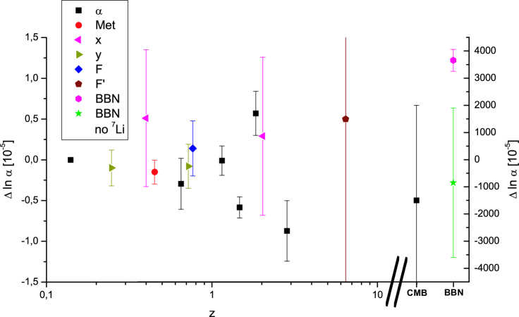
Figure 1: Variations for varying $\alpha$ alone. Only observations constraining $\alpha$ variation are shown; the BBN fit including ⁷Li is poor ($\chi^{2}/\nu\geq 7.8/2$) hence we also display a conservative bound from ⁴He and D abundances neglecting ⁷Li.

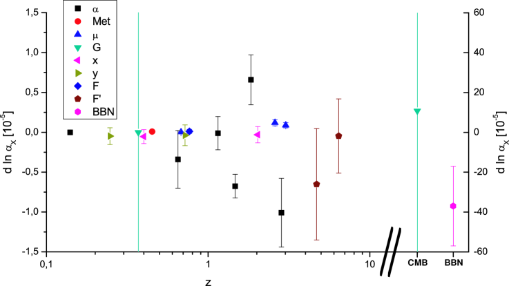
Figure 2: Variations for scenario 2; BBN bounds are $2\sigma$ bounds.

3.2 Scenario 1: Varying gravitational coupling

In this scenario we have only $d_{M}$ nonvanishing,

$$d_{H}=d_{S}=d_{X}=0,$$ (50)

therefore

$$\Delta\ln\frac{M_{X}}{M_{\rm P}}=\frac{1}{2}\Delta\ln G\Lambda_{c}^{2}.$$ (51)

We find that there is no value of $\Delta\ln G\Lambda_{c}^{2}$ for which BBN is consistent with the three observed abundances within $2\sigma$. The best fit values are $\chi^{2}/\nu\geq 7.7$ for no variation of $m_{N}/M_{\rm P}$ at CMB and $\chi^{2}/\nu\geq 5.9$ if the variation of $m_{N}/M_{\rm P}$ has the same size at BBN and CMB. Assuming that the discrepancy in the ⁷Li abundance is due to some other effect, we find the allowed region of variation of $G$ at BBN under which primordial D and ⁴He abundance lie within the observed range at $1\sigma$ ($2\sigma$),

$$-5\%\;(-13\%)\leq\Delta\ln G\Lambda_{c}^{2}\leq 12\%\;(22\%)$$ (52)

If the variation of $m_{N}/M_{\rm P}$ has the same size at BBN and CMB one finds

$$-4\%\;(-11\%)\leq\Delta\ln G\Lambda_{c}^{2}\leq 10\%\;(16\%).$$ (53)

The bounds on time variation of $G\Lambda_{c}^{2}$ are much weaker than for many other varying couplings. This scenario also predicts a vanishing value of $\eta$ in Eötvös experiments. Thus, to any one of the following scenarios we may add an additional nonzero $d_{M}$ of similar size to $d_{X}$, $d_{H}$ or $d_{S}$ without changing the results significantly.

3.3 Scenario 2: Varying unified coupling

In the first GUT scenario without SUSY we consider the case when only $d_{X}$ is nonvanishing,

$$d_{X}=1,\qquad d_{H}=d_{S}=d_{M}=0,\qquad\alpha_{X}=1/40.$$ (54)

Within a supersymmetric theory the same relations will apply except that $\alpha_{X}=1/24$ and the variations of observables are scaled by a factor $24/40$ relative to $\Delta\ln\alpha_{X}$: we designate this as Scenario 2S. In both cases we find here

$$\frac{\Delta\ln\mu}{\Delta\ln\alpha}\simeq 27.$$ (55)

It is then highly unlikely for the nonzero M$\alpha$ result for variation of $\alpha$ to coexist with the determination of $\mu$ at redshift around $3$ [37], even if the latter is interpreted as an upper bound on the absolute size of variation [38].

For the BBN fit, we find without SUSY (excluding modifications of the baryon fraction $\eta$ due to varying $m_{N}$) no range of values fitting at $1\sigma$ level ($\chi^{2}/\nu\geq 2.3$). At $2\sigma$ the abundances, including ⁷Li, become consistent for the range

$$-5.7\times 10^{-4}\leq\Delta\ln\alpha_{X}\leq-1.7\times 10^{-4}\qquad(2\sigma).$$ (56)

If one includes a variation of $m_{N}$ at the time of CMB with the same magnitude as at BBN the result remains unchanged ($\chi^{2}/\nu\geq 2.45$), with the same $2\sigma$ range. For this scenario we may consider a nonzero variation at BBN, but more recent probes must all be viewed as increasingly tight null bounds.

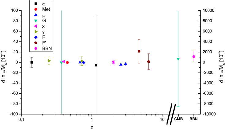
Figure 3: Variations for scenario 3; BBN bounds are $2\sigma$. Note that due to the very large ratio $\Delta\ln\mu/\Delta\ln\alpha$ in this scenario, points indicating any nonzero variation of $\alpha$ fall well outside the range of the graph.

3.4 Scenario 3: Varying Fermi scale

In this scenario we consider the case when the variation arises solely from a change in the Higgs expectation value relative to the unified scale, thus only $d_{H}$ is nonzero:

$$d_{H}=1,\quad d_{S}=d_{M}=d_{X}=0,\qquad\alpha_{X}=1/40.$$ (57)

This scenario implies

$$\frac{\Delta\ln\mu}{\Delta\ln\alpha}=-325.$$ (58)

Whether we interpret the determination of $\mu$ [37] as a detection or an upper bound, any variation in $\alpha$ at large redshift case should be orders of magnitude smaller than current observational sensitivity.

We find for BBN including ⁷Li ($\nu=2$) no $1\sigma$ range ($\chi^{2}/\nu\geq 1.95$) but

$$6\times 10^{-3}\leq\Delta\ln\langle\phi\rangle/M_{X}\leq 22\times 10^{-3}\qquad(2\sigma).$$ (59)

A variation of $m_{N}$ at the time of CMB with the same magnitude as at BBN does not change this result.

3.5 Scenario 4: Varying Fermi scale and SUSY-breaking scale

This scenario corresponds to scenario 3, but includes supersymmetry and assumes that the mass-generating mechanism for SM particles and their superpartners gives rise to the same variation:

$$d_{M}=d_{X}=0,\quad d_{S}=d_{H}=1,\qquad\alpha_{X}=1/24.$$ (60)

We find here

$$\frac{\Delta\ln\mu}{\Delta\ln\alpha}=-21.5,$$ (61)

such that again the claimed nonzero variations in $\alpha$ and $\mu$ cannot be compatible and the variation in $\alpha$ at redshift $3$ must be below current sensitivities. We demonstrate this in Fig. 4, where we show for this scenario the bounds on the variable $d_{H}l=\Delta\ln(\langle\phi\rangle/M_{X})$ that arise from various observations. Since we have only one free variable we can plot all observations simultaneously as a function of redshift. Inspection “by eye” permits to judge if a smooth and monotonic evolution of $d_{H}l$ is consistent or not.

We find for BBN including ⁷Li($\nu=2$) no $1\sigma$ fit ($\chi^{2}/\nu\geq 1.60$), while at $2\sigma$

$$1.25\times 10^{-2}\leq\Delta\ln\langle\phi\rangle/M_{X}\leq 5.4\times 10^{-2}\qquad(2\sigma).$$ (62)

If one includes a variation of $m_{N}$ at the time of CMB with the same magnitude as at BBN the allowed range becomes slightly restricted ($\chi^{2}/\nu\geq 1.72$),

$$1.20\times 10^{-2}\leq\Delta\ln\langle\phi\rangle/M_{X}\leq 4.9\times 10^{-2}\qquad(2\sigma).$$ (63)

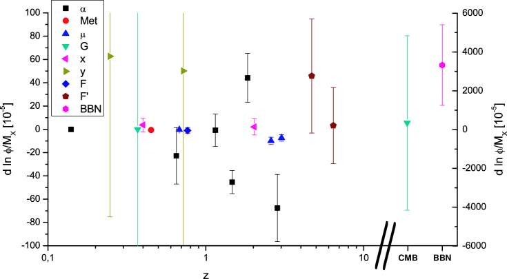
Figure 4: Variations for scenario 4; BBN bounds are $2\sigma$

3.6 Scenario 5: Varying unified coupling and Fermi scale

In this scenario we study a combined variation of the unified coupling and the Higgs expectation value:

$$d_{M}=d_{S}=0,\quad d_{X}=1,\quad d_{H}=\tilde{\gamma}d_{X},\qquad\alpha_{X}=1/40.$$ (64)

The parameter $\tilde{\gamma}$ can be related to the parameter $\gamma\equiv\frac{\Delta\ln\langle\phi\rangle/M_{X}}{\Delta\ln\Lambda_{c}/M_{X}}$ which was introduced in [1] via

$$\gamma=\tilde{\gamma}\left(\frac{2\pi}{9\alpha_{X}}+\frac{2}{9}\tilde{\gamma}\right)^{-1}.$$ (65)

In [1] we examined the cases $\gamma=(0,1,1.5)$ which correspond to $\tilde{\gamma}=(0,36,63)$. Here we find that the best BBN fit is reached for $\tilde{\gamma}\approx 50$ with $\chi^{2}/\nu=1.45$. Note that we have the freedom to adjust $\tilde{\gamma}$ such that nonzero variations of $\alpha$ and $\mu$ at redshift $\simeq 3$ are consistent with each other. We have

$$\frac{\Delta\ln\mu}{\Delta\ln\alpha}=\frac{23.2-0.65\tilde{\gamma}}{0.865+0.002\tilde{\gamma}}\,.$$ (66)

We choose for illustration $\tilde{\gamma}=42$, for which

$$\Delta\ln\mu=-5.6\,\Delta\ln\alpha$$ (67)

and the $2\sigma$ contour for BBN is

$$7.5\times 10^{-4}\leq\Delta\ln\alpha_{X}\leq 28\times 10^{-4}.$$ (68)

For a variation of $m_{N}$ at the time of CMB with the same magnitude as at BBN the fit becomes worse ($\chi^{2}/\nu\geq 1.68$). However, a $2\sigma$ fit to BBN is obtained over a wide range of $0\leq\tilde{\gamma}\leq 26$ (negative $\Delta\ln\alpha_{X}$) and $40\leq\tilde{\gamma}<\infty$ (positive $\Delta\ln\alpha_{X}$).

Assuming that the apparent ⁷Li mismatch at BBN is due to systematic astrophysical effects, we may bound $\alpha_{X}$ with only D and ⁴He abundances. Here we find at $1\sigma$

$$-5.5\times 10^{-4}\leq\Delta\ln\alpha_{X}\leq 1.44\times 10^{-3}$$ (69)

In Fig. 5 we again plot simultaneously all observations for this scenario. This shows that the bound from BBN including ⁷Li is not consistent with the claimed nonzero variations of $\alpha$ and $\mu$ for a monotonic evolution over $z$.

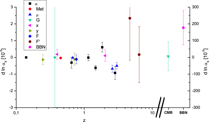
Figure 5: Variations for scenario 5, $\tilde{\gamma}=42$; BBN bounds are $2\sigma$

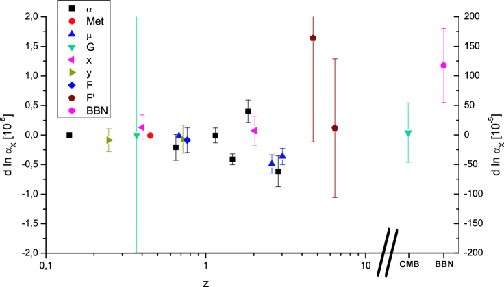
Figure 6: Variations for scenario 6, $\tilde{\gamma}=70$; BBN bounds are $2\sigma$

3.7 Scenario 6: Varying unified coupling and Fermi scale with SUSY

In this scenario we study a combined variation of the unified coupling and the Higgs v.e.v. including SUSY, where as in Scenario 4 we tie the variations of the superpartner masses and Fermi scale together:

$$d_{M}=0,\quad d_{X}=1,\quad d_{S}\simeq d_{H}=\tilde{\gamma}d_{X},\qquad\alpha_{X}=1/24.$$ (70)

Now the relation to $\gamma$ is modified as

$$\gamma=\tilde{\gamma}\left(\frac{2\pi}{9\alpha_{X}}+\frac{2}{3}\tilde{\gamma}\right)^{-1}$$ (71)

One may again adjust $\tilde{\gamma}$ to make nonzero variations in $\alpha$ and $\mu$ self-consistent. With

$$\frac{\Delta\ln\mu}{\Delta\ln\alpha}=\frac{14-0.28\tilde{\gamma}}{0.52+0.013\tilde{\gamma}}\,,$$ (72)

we find that a good fit to BBN is obtained over a large range of $\tilde{\gamma}$, ranging from $\tilde{\gamma}=100$ to infinity with minimal $\chi^{2}/\nu=1.45$. This shows that the main effect in the SUSY model comes from the variation of the Higgs v.e.v. Including a variation of $m_{N}$ at the time of CMB with the same magnitude as at BBN the fits gets worse ($\chi^{2}/\nu\geq 1.8$). A $2\sigma$ fit can be obtained for $0\leq\tilde{\gamma}\leq 28$ (for negative $\Delta\ln\alpha_{X}$ at BBN) and for $58\leq\tilde{\gamma}<\infty$ (positive $\Delta\ln\alpha_{X}$).

First, we study the case $\tilde{\gamma}=70$ for which

$$\Delta\ln\mu=-3.9\Delta\ln\alpha\qquad(\tilde{\gamma}=70)$$ (73)

and BBN is fit with a $2\sigma$ range

$$5.5\times 10^{-4}\leq\Delta\ln\alpha_{X}\leq 18\times 10^{-4}.$$ (74)

Neglecting ⁷Li, we obtain a $1\sigma$ bound from BBN

$$-3.5\times 10^{-4}\leq\Delta\ln\alpha_{X}\leq 9.3\times 10^{-4}.$$ (75)

Secondly, we study the case $\tilde{\gamma}=25$ where

$$\Delta\ln\mu=8.3\Delta\ln\alpha\qquad(\tilde{\gamma}=25),$$ (76)

and where the $2\sigma$ contour for BBN is

$$-13\times 10^{-4}\leq\Delta\ln\alpha_{X}\leq-7\times 10^{-4}.$$ (77)

In this second case the Murphy $\alpha$ measurement and BBN point into the same direction. The difference between the two values of $\tilde{\gamma}$ can be seen from a comparison of Figs. 6 and 7.

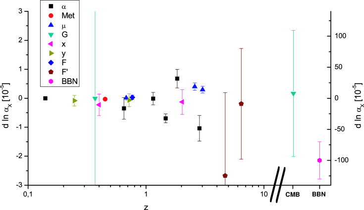
Figure 7: Variations for scenario 6, $\tilde{\gamma}=25$; BBN bounds are $2\sigma$

4 Epochs and evolution factors

4.1 Epochs

In this section we group the information contained in Tables 1-3 and figures 1-7 into different cosmological epochs. This produces a first quantitative estimate of the possible time evolution for the various unified scenarios. The choice of epochs is somewhat arbitrary. Two epochs are singled out by events in early cosmology, namely the last scattering surface of CMB, and BBN. The very recent epoch comprises present day laboratory experiments and the Oklo natural reactor, for which a linear interpolation to the present rate of varying couplings seems reasonable. We further divide the observations at intermediate redshift into three epochs.

• Epoch 1: Today until Oklo
  Contains Oklo and laboratory measurements. For the laboratory measurements, we extrapolate the rate of change of the couplings to finite changes at the redshift $z=0.14$ ($t=1.8\times 10^{9}\,$y) of the Oklo event.

• Epoch 2: $0.2\leq z\leq 0.8$
  Contains absorption spectra and isotopic abundance measurements in meteorites. We chose a boundary $z=0.8$ since the Murphy dataset [28] has relatively few systems around this redshift, making a natural division.

• Epoch 3: $0.8\leq z\leq 2.4$
  Contains several absorption spectra measurements. The end of the Tzanavaris dataset [42] sets the cut at $z=2.4$.

• Epoch 4: $2.4\leq z\leq 10$
  Contains absorption spectra measurements and bounds on $G$ from neutron stars.

• Epoch 5: CMB, $z\approx 1100$

• Epoch 6: BBN, $z\approx 10^{10}$

4.2 Evolution factors

We define “evolution factors” $l_{n}$ for epochs $n=1,\ldots,6$ by

$$\Delta\ln G_{k,n}=d_{k}l_{n}.$$ (78)

For each unification scenario we will proceed to a quantitative estimate of $l_{n}$, shown in Table 4. The usefulness of considering the evolution factors $l_{n}$ is that the unknown (and possibly not monotonic) behaviour of the mechanism driving the coupling variations is rolled into a finite number of parameters. For a monotonic behaviour they satisfy $l_{n}<l_{p}$ whenever $z_{n}<z_{p}$. The basic assumption remains the proportionality $\Delta\ln G_{k}(z_{n})=d_{k}l(z_{n})=d_{k}l_{n}$, with constant unification coefficients $d_{k}$ independent of the epoch. The normalization of $l_{n}$ is arbitrary, and we take for scenarios 2, 5 and 6

$$l_{n}=\Delta\ln\alpha_{X,n},$$ (79)

while for scenarios 3 and 4 we take

$$l_{n}=\Delta\ln(\langle\phi\rangle/M_{X})_{,n}.$$ (80)

For each epoch and scenario, we compute the evolution coefficients $l_{n}$ as a weighted average over the measurements in the epoch. The representative redshift $z_{n}$ is the average over the redshifts of observations inside the corresponding epoch. It is shown together with the resulting values for $l_{n}$ in table 4. This table summarizes our results under the assumption of proportionality.

Rates of time variation in the present epoch

For Epoch 1 we incorporate the laboratory measurements for rates of varying couplings by linear extrapolation in time to the Oklo redshift $z_{1}=0.14$. The logarithmic time derivatives may be approximated by linear interpolation

$$\frac{\dot{G}_{k}}{G_{k}}=\partial_{t}\ln G_{k}\simeq-\frac{d_{k}l_{1}}{t_{0}-t_{1}},$$ (81)

where $t_{1}=1.8\times 10^{9}$y is the time corresponding to the redshift $z_{1}=0.14$.

Method of averaging

We evaluate the weighted average using all values listed in table 1. This procedure may be quite problematic, since sometimes different observations are in manifest contradiction. We take the attitude that, given the possible presence of systematic effects both in spectroscopic determinations of nonzero coupling variations and in the primordial ⁷Li abundance, a viable model need not fit all data points. However, even if any given nonzero claimed variation is actually due to systematic error, we still expect the size of the error to be comparable to the size of the claimed variation. Thus, such claims are most conservatively interpreted as bounds on the absolute magnitude of variation. The surviving nonzero variation(s), in addition to the null bounds at other epochs, define a set of evolution factors which must be satisfied by any explicit model of evolution.

For some scenarios we therefore also evaluate the evolution factors that are obtained by considering that some of the claimed observations of nonzero variation may instead be due to an underestimated systematic error. These alternative evolution factors are given in square brackets, corresponding to the following replacements:
Scenario 5, $\tilde{\gamma}=42$: Neglecting ⁷Li-abundance at BBN
Scenario 6, $\tilde{\gamma}=70$: Neglecting ⁷Li-abundance at BBN
Scenario 6, $\tilde{\gamma}=25$: Replacing the $\mu$ measurements of [37] by the conservative upper bound of [38].
In the case where $\alpha$ alone varies, since the fit including ⁷Li is poor we calculate a $2\sigma$ range using observational central values and errors of D and ⁴He abundances given in [1].

Epoch	1	2	3	4	5	6
$z_{n}$	0.14	0.53	1.6	3.8	$10^{3}$	$10^{10}$
Scenario	$l_{1}\times 10^{6}$	$l_{2}\times 10^{6}$	$l_{3}\times 10^{5}$	$l_{4}\times 10^{5}$	$l_{5}\times 10^{4}$	$l_{6}\times 10^{3}$
$\alpha$ only	$-0.01\pm 0.06$	$-1.1\pm 1.0$	$-0.26\pm 0.10$	$-0.85\pm 0.37$	$-150\pm 350$	$5\pm 34$
2	$-0.1\pm 0.1$	$0.04\pm 0.03$	$-0.15\pm 0.08$	$0.10\pm 0.03$	$0.9\pm 14$	$-0.37\pm 0.20$
3	$4.1\pm 4.8$	$-1.5\pm 1.2$	$0.42\pm 3.3$	$-3.6\pm 0.9$	$69\pm 920$	$14\pm 8$
4	$3.9\pm 8.5$	$-3.4\pm 2.7$	$-8.4\pm 5.1$	$-8.7\pm 2.1$	$31\pm 450$	$33\pm 21$
5,	$-0.02\pm 0.18$	$-0.24\pm 0.18$	$-0.25\pm 0.10$	$-0.61\pm 0.13$	$0.6\pm 8.6$	$1.7\pm 1.1$
($\tilde{\gamma}=42$)						[$0.4\pm 1.0$]
6,	$-0.02\pm 0.12$	$-0.10\pm 0.07$	$-0.17\pm 0.07$	$-0.44\pm 0.10$	$0.3\pm 5.0$	$1.2\pm 0.6$
($\tilde{\gamma}=70$)						[$0.3\pm 0.6$]
6,	$-0.12\pm 0.18$	$0.04\pm 0.12$	$-0.30\pm 0.11$	$0.29\pm 0.08$	$0.7\pm 10$	$-1\pm 0.3$
($\tilde{\gamma}=25$)				[$-0.43\pm 0.28$]

Table 4: Redshifts and evolution factors for each epoch, for the scenarios defined in section 3. In the first row the values of $l_{n}$ give the fractional variation of $\alpha$; in Scenarios 2, 5 and 6 that of $\alpha_{X}$; and in 3 and 4 that of $\langle\phi\rangle/M_{X}$. Values in brackets give, for BBN ($l_{6}$) the evolution factors neglecting ⁷Li; or for $l_{4}$, the evolution factor with the $\Delta\mu/\mu$ value of [37] substituted by that of [38].

4.3 Monotonic evolution with unification

Here we briefly summarize whether the unified scenarios we consider can be consistent with a monotonic evolution of the single underlying varying parameter, based on the evolution factors $l_{i}$ found in Table 4.

Varying $\alpha$ only

Although variation of $\alpha$ alone does not help to account for deviation of BBN abundances from standard theory, or for any nonzero variation of $\mu$, the cosmic history is interesting due to the significant nonzero value in Epochs 3 and 4. The Oklo bound in Epoch 1 restricts the present time variation to $3.7\times 10^{-17}\,{\rm y}^{-1}$ (assuming no acceleration of $\partial_{t}\alpha$).

Scenario 2

Scenario 2 favours a negative variation of $\alpha_{X}$ at BBN, and a negative variation may also fit the M$\alpha$ results. However, the Reinhold $\mu$ measurement indicates a positive, but much smaller, variation. We keep the R$\mu$ results, which dominate the weighted average due to their small error on $\Delta\ln\alpha_{X}$, to obtain $l_{4}$. The ratio $\Delta\ln\mu/\Delta\ln\alpha=27$ makes this scenario unlikely to fit the reported signal of nonzero $\Delta\alpha$.

Scenario 3

In scenario 3 a positive variation of $\langle\phi\rangle/M_{X}$ is favoured by BBN. The high ratio $\Delta\ln\mu/\Delta\ln\alpha\simeq-325$ makes the bounds obtained on a variation of $\mu$ strongly inconsistent with the claimed size of variation of $\alpha$. We keep the Reinhold et al. values to obtain $l_{4}$, which again dominate the results.

Scenario 4

In this scenario, the ratio $\Delta\ln\mu/\Delta\ln\alpha=-22$ is again large and makes any observation of significant nonzero $\Delta\ln\alpha$ unlikely. Both the M$\alpha$ and the R$\mu$ measurements point in opposite direction to BBN; however the two spectroscopic observations are also inconsistent with each other, within the scenario. Again, we keep the R$\mu$ results which dominate the determination of $l_{4}$ due to the small error.

Scenario 5, $\tilde{\gamma}=42$

In this scenario the variation of $\alpha_{X}$ favoured by BBN is positive ($l_{6}=(1.7\pm 1)\times 10^{3}$), however both nonzero variations from spectroscopic data M$\alpha$ and R$\mu$ require negative variations. With $\Delta\ln\mu/\Delta\ln\alpha=-6$ the spectroscopic measurements appear consistent with each other. Hence one would require some non-monotonic evolution to fit nonzero variations both at BBN and at moderate $z$. Thus in Table 4 we have also evaluated $l_{6}$ using only the constraints given by D and ⁴He (in brackets).

Scenario 6, $\tilde{\gamma}=70$

As in the preceding scenario, BBN favours a positive variation in $\alpha_{X}$, but M$\alpha$ and R$\mu$ favour negative. Again, Fig. 6 may suggest a non-monotonic evolution. Fitting to BBN including ⁷Li we would obtain $l_{6}=(1.2\pm 0.6)\times 10^{-3}$; table 4 also displays in brackets the value of $l_{6}$ obtained from D and ⁴He bounds only.

Scenario 6, $\tilde{\gamma}=25$

In this scenario, both BBN and the M$\alpha$ signal favour a negative variation of $\alpha_{X}$, whereas the R$\mu$ observations point towards a positive variation. Following the argument of Wendt et al. [38], we substitute the R$\mu$ value by the null constraint $|\Delta\mu/\mu|\leq 2.5\times 10^{-5}$ [38] to obtain the bracketed value of $l_{4}$ in Table 4. In this scenario the evolution factors show a crossover from negligible variation at low redshift, to strong and monotonically increasing negative variation at $z\approx 2$.

4.4 Tension between the ⁷Li problem and variation of $\mu$

Measurements of the primordial ⁷Li abundance show that the BBN abundance needs to decrease below the standard value to fit the observations, whereas the Reinhold $\mu$ measurement indicates $\mu$ to increase at $z\simeq 3$. We find that for all our unification scenarios the sign of the dependence on the fundamental parameter is the same for $\mu$ and ⁷Li. Moreover, the coefficients of this dependence are nearly identical up to a common factor; hence the induced variations for $\mu$ and ⁷Li point in the same direction, in contradiction to the tendency inferred from the observations. For example, for scenario 5 we find

$$\Delta\ln\mu =(23.2-0.65\tilde{\gamma})\Delta\ln\alpha_{X},$$

$$\Delta\ln\mbox{${{}^{7}}$Li} =(1692-49\tilde{\gamma})\Delta\ln\alpha_{X}.$$ (82)

These expressions change sign at $\tilde{\gamma}=35.7$ and $34.5$, respectively. For a monotonic evolution, there is no possibility to have both a significant variation of $\mu$ and a variation of opposite sign in the ⁷Li abundance. (In the regime $\tilde{\gamma}\approx 35$ there is no $2\sigma$ fit to BBN.) A similar result can be found for scenario 6 (including the SUSY partner mass dependence, which shows the same sort of degeneracy). Note that scenario 2 and 3 are just limiting cases of scenarios 5 and 6.

The main reason for this behaviour is that variations of ⁷Li and $\mu$ are dominated by the variations of $\hat{m}/\Lambda_{c}$ and $m_{e}/\Lambda_{c}$, respectively, with the same sign of prefactor. This degeneracy can be broken if $m_{e}$ varies differently from the quark masses, a possibility that we do not consider in this paper. For our scenarios with constant $\hat{m}/m_{e}$, the conflict between a monotonic time evolution and the $\mu$- and ⁷Li-observations is reflected in the opposite signs of $l_{4}$ and $l_{6}$.

This observational tension for monotonic behaviour is clearly depicted in Fig. 8, where we plot simultaneously the averaged observational values of evolution factors $l_{i}/\ln(1+z_{i})$, normalized to $l_{4}/\ln(1+z_{4})$. For Scenario 6, $\tilde{\gamma}=25$, we also display the result obtained by substituting the Wendt et al. value of $\mu$ variation for that of [37].

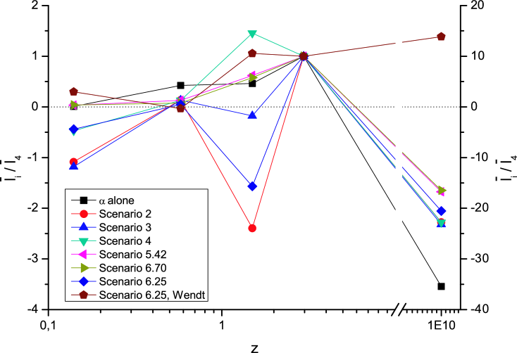
Figure 8: Normalised evolution factors $\bar{l}_{i}/\bar{l}_{4}$ for each scenario, where $\bar{l}_{i}\equiv l_{i}/\ln(1+z_{i})$.

The factor $\ln(1+z_{i})$ is introduced as a convenient normalization to avoid compressing the scale of variations excessively in recent epochs. For the purpose of a quick inspection we have omitted the error bars, which are of course necessary for a quantitative interpretation.

4.5 Special values of $\tilde{\gamma}$

In Scenarios 5 and 6 there is a value of $\tilde{\gamma}$ for which $\Delta\ln\langle\phi\rangle/\Lambda_{c}$ vanishes. For these values, Standard Model physics undergoes an overall multiplicative shift of energy scale under variation of $\alpha_{X}$, up to variations of perturbative, dimensionless couplings: specifically the Yukawa couplings (whose variation we have generally neglected) and $\alpha$. The significant observable effects arising from variation of SM fermion masses relative to $\Lambda_{c}$, which dominate in most unified scenarios, are largely absent, and the low-energy phenomenology is very similar to the case of varying $\alpha$ only. In particular the ⁷Li problem at BBN is not addressed and the variation of $\mu$ is smaller than that of $\alpha$.

The required values are $\tilde{\gamma}=2\pi/7\alpha_{X}\simeq 36$ in the case without SUSY ($\alpha_{X}\simeq 1/40$); or $\tilde{\gamma}=2\pi/3\alpha_{X}\simeq 50$ with SUSY ($\alpha_{X}\simeq 1/24$) when the superpartner masses vary with the Fermi scale, $d_{S}=d_{H}=\tilde{\gamma}d_{X}$. From a low-energy point of view these values appear as fine-tuning, however it is conceivable that they would arise from some specific mechanisms of electroweak symmetry-breaking or SUSY-breaking.

5 Summary / Conclusions

Within Grand Unified Theories, different measurements of the variation of fundamental constants can be consistently reduced to a variation of a few “unification parameters”, namely the unification scale $M_{X}/M_{\rm P}$, gauge coupling $\alpha_{X}$, the Fermi scale $\langle\phi\rangle/M_{X}$ and SUSY-breaking masses $\tilde{m}/M_{X}$. We define various GUT-scenarios for varying couplings by the assumption of proportionality of fractional variations of the unification parameters.

Assuming that couplings really vary, this is a way of excluding such GUT scenarios by demanding consistency of the implied variations. The assumption of proportionality permits us to project all observations into constraints on a common evolution factor $l(z)$ for each scenario. We show that different GUT scenarios yield different time evolutions of $l(z)$ assuming that certain claimed measurements of varying constants are correct. We confirm that “simple” models which have only one fundamental parameter varying ($\alpha_{X}$ or $\langle\phi\rangle/M_{X}$) result in inconsistent variations. However, combined variations of these two parameters, as described in scenarios 5 and 6, lead to results more consistent with the possible quintessence-induced time variations of fundamental couplings which we investigate in [7].

Specifically, one may ask whether the claimed observations of variations in $\alpha$ [28] and $\mu$ [37] are mutually consistent, and whether they are consistent with an explanation of the apparent primordial ⁷Li-depletion by varying couplings. Within a hypothesis of constant Yukawa couplings, which results in identical fractional variations of all quark and lepton masses, we investigated arbitrary variations of $\alpha_{X}$, $\langle\phi\rangle/M_{X}$ and $M_{X}/M_{\rm P}$. For scenarios with supersymmetry we also assumed that the SUSY-breaking masses vary proportional to $\langle\phi\rangle$, but the effect of such a variation only appears at higher order and is probably not crucial.

We have not found a scenario with a monotonic time evolution $l(z)$ that makes all three signals or hints of variation mutually consistent. A monotonic evolution requires either to discount one of the “signals” by substantially increasing its uncertainty, or to alter our assumptions by including additional time variation of some Yukawa couplings.

Our investigation shows how the variations of different couplings in the Standard Model may be compared. If the observational situation becomes clearer and at least one nonzero time variation is established, such methods may be used for new tests of the idea of grand unification.

Note added

Shortly before the completion of this paper a new determination of the variation of $\mu$ appeared [67] reporting a reanalysis of spectra from the same two H₂ absorption systems as [37], and adding one additional system at $z\simeq 2.8$. The results of the new analysis are not consistent with the previous claim indicating a nonzero variation, either considering all three systems or the two previously considered. The stringent null bound of the new analysis, $\Delta\mu/\mu=(2.6\pm 3.0)\times 10^{-6}$, would disfavour all scenarios except those where the fractional variation of $\mu$ was of the same order as or smaller than that of $\alpha$. This would require us to approach the “special”, apparently fine-tuned values of $\tilde{\gamma}$ discussed in Section 4.5, for which $\mu$ variation (and any deviation from the standard ⁷Li abundance at BBN) are suppressed.

Acknowledgements

We acknowledge useful discussions with M. Pospelov, R. Trotta, P. Molaro, P. Avelino, J. Berengut and V. Flambaum, and invaluable correspondence and discussions with M. Murphy. T. D. is supported by the Impuls- and Vernetzungsfond der Helmholtz-Gesellschaft.

Appendix Appendix A Effect of “varying constants” at CMB and $\eta$

In our previous work on BBN we used the WMAP determination of the baryon number density parameter $\eta\equiv n_{B}/n_{\gamma}$ directly to reduce by one the number of unknown parameters. However, we should also consider the effect of possible variations of $G_{k}$ at the epoch of CMB decoupling. This question has distinct aspects: first, can the CMB alone or combined with various other cosmological observations give useful bounds on the values of fundamental parameters at this epoch? Second, how do the possible variations affect the determination of $\eta$?

It would not be appropriate to give an extended discussion of CMB bounds on fundamental variations here; the subject has already been treated [25] at length. Bounds tend to depend strongly on the values taken by cosmological parameters which are not at present well known through independent measurements: in other words there is considerable degeneracy. Fundamental parameters affecting the CMB are the proton and electron masses, the gravitational constant and the fine structure constant, as well as the mass of any dark matter particle present. In Planck units, these reduce to the particle masses and $\alpha$. The relevant cosmological parameters are the amplitude, spectral index (and possible running, etc.) of primordial perturbations; the baryon, dark matter and dark energy (cosmological constant, etc.) densities normalised to the critical density; the Hubble constant; and the reionization optical depth. Of these, the baryon density $\Omega_{b}h^{2}$ will vary linearly with the proton mass in Planck units, for a fixed baryon-to-photon ratio $\eta$. Conversely, given a measurement of $\Omega_{b}h^{2}$, the correct value of $\eta$ varies inversely with the proton mass. The conversion factor between $\Omega_{b}h^{2}$ and $\eta_{10}\equiv 10^{10}\eta$ is then $273.9(m_{p}\sqrt{G})_{|0}(m_{p}\sqrt{G})^{-1}\simeq 273.9(1-\Delta\ln(m_{N}/M_{\rm P})_{|\rm CMB})$, where we approximate the proton and neutron masses by their average $m_{N}$.

If, therefore, we allow the proton mass (or the gravitational constant, in QCD units) to vary arbitrarily at the CMB epoch, $\eta$ is undetermined by WMAP and we must consider it as an extra free parameter or try to impose independent cosmological bounds. However, we impose that the size of variations away from the present value of $m_{p}/M_{\rm P}$ is a monotonically decreasing function of time: thus $\Delta\ln(m_{N}/M_{\rm P})_{|\rm CMB}\leq\Delta\ln(m_{N}/M_{\rm P})_{|\rm BBN}$. Hence we would have a self-consistent treatment of this parameter if the secondary discrepancies in primordial abundances due to an incorrectly estimated $\eta$ were smaller than the primary effect of varying $m_{N}/M_{\rm P}$ at BBN. The relevant results of our previous analysis

$$\frac{\partial\ln({\rm D/H},Y_{\rm p},\mbox{${{}^{7}}$Li/H})}{\partial\ln(m_{N}/M_{\rm P})_{|\rm BBN}} = \ (1.88,0.72,-1.14),$$

$$\frac{\partial\ln({\rm D/H},Y_{\rm p},\mbox{${{}^{7}}$Li/H})}{\partial\ln\eta}=- \frac{\partial\ln({\rm D/H},Y_{\rm p},\mbox{${{}^{7}}$Li/H})}{\partial\ln(m_{N}/M_{\rm P})_{|\rm CMB}} = \ (-1.6,0.04,2.1)$$ (83)

are derived in QCD units where the strong coupling scale $\Lambda_{c}$ is constant, and where we neglect small contributions to the nucleon mass $m_{N}$ and take it proportional to $\Lambda_{c}$. The first relation, derived at a fixed value of $\eta=6.1\times 10^{-10}$ (WMAP3 [68]) led to the bound $-0.095\leq\Delta\ln(m_{N}/M_{\rm P})_{|\rm BBN}\leq+0.05$, where the main sensitivity to this variation is due to helium-4 ($Y_{\rm p}$). Since this abundance is insensitive to changes in $\eta$, we postulate also that $-0.095\leq\Delta\ln(m_{N}/M_{\rm P})_{|\rm CMB}\leq 0.05$.

The resulting errors in the (standard) BBN abundances due to a possibly misestimated $\eta$ are then

$$\delta\ln({\rm D/H},Y_{\rm p},\mbox{${{}^{7}}$Li/H})=(\{-0.15,0.08\},\{-0.002,0.004\},\{-0.10,+0.20\})$$ (84)

to be compared with observational errors of

$$\sigma_{\rm D}/(\mbox{D/H})\simeq 0.4/2.6\simeq 0.15$$

$$\sigma_{\rm 4He}/Y_{\rm p}\simeq 0.009/0.25\simeq 0.04$$

$$\sigma_{\rm 7Li}/(\mbox{${{}^{7}}$Li/H})\simeq 0.5/4.5\simeq 0.1,$$ (85)

where we take the standard BBN ⁷Li abundance $4.5\times 10^{-10}$ as central value. Hence the variation of $m_{N}/M_{\rm P}$ at the CMB epoch and consequent rescaling of $\eta$ may in principle have significant consequences for deuterium and lithium abundances in BBN. It may be appropriate to take $\Delta\ln(m_{N}/M_{\rm P})_{|\rm CMB}$ as an independent variable in the analysis of BBN variations. The maximum effect due to rescaling of $\eta$ would occur when $\Delta\ln(m_{N}/M_{\rm P})_{|\rm CMB}$ = $\Delta\ln(m_{N}/M_{\rm P})_{|\rm BBN}$, giving a total sensitivity of

$$\frac{\partial\ln({\rm D/H},Y_{\rm p},\mbox{${{}^{7}}$Li/H})}{\partial\ln(m_{N}/M_{\rm P})_{|\rm BBN,CMB}}=(3.48,0.68,-3.24).\\$$ (86)

Appendix Appendix B The ⁸Be resonance

The ⁷Be$+n\rightarrow$⁷Li$+p$ reaction is the main channel for destruction of ⁷Be during BBN. If this reaction was not present, the final ⁷Li abundance predicted by standard BBN would be considerably higher:

$$\mbox{${{}^{7}}$Li/H}=4.5\times 10^{-10}\rightarrow\ \ \sim 14\times 10^{-10}.$$

The high cross section of this reaction is due to a strong ⁸Be resonance which sits at about the energy of both ⁷Be$+n$ and ⁷Li$+p$ [69]. For the reaction to continue to operate efficiently, it is important that the resonance remains near these ⁷Be / ⁷Li energy levels. We will argue here that, given the size of coupling variations relevant for our paper, this is indeed the case.

In [1] we estimated the dependence of nuclear binding energies on the pion mass by

$$\frac{\partial B_{i}}{\partial m_{\pi}}=f_{i}(A_{i}-1)\frac{B_{\rm D}}{m_{\pi}}r\simeq-0.13f_{i}(A_{i}-1),$$ (87)

taking $r\simeq-8$. The constants $f_{i}$ are expected to be of order unity, but will differ between light nuclei due to peculiarities of the shell structure. Our normalization corresponds to $f_{\rm D}=1$. We are then concerned with the relative changes of the ⁷Be and ⁷Li binding energies and the energy of the ⁸Be resonance, whose dependence we will estimate in an analogous way with a constant of proportionality $f^{\prime}_{8}$. Then

$$\Delta B_{\rm 7Be} = -9.1\,\mbox{MeV}\times 6f_{\rm 7Be}\,\Delta\ln\hat{m},$$

$$\Delta E_{\rm 8Be^{*}} = -9.1\,\mbox{MeV}\times 7f^{\prime}_{8}\,\Delta\ln\hat{m},$$

$$\Delta B_{\rm 7Li} = -9.1\,\mbox{MeV}\times 6f_{\rm 7Li}\,\Delta\ln\hat{m},$$ (88)

recalling that $m_{\pi}\propto\hat{m}^{1/2}$. In [70] the sum of the neutron and proton widths of the ⁸Be resonance is given as approximately $1.6\,\mbox{MeV}$ thus for the ⁸Be-destroying reaction to remain effective we require at least

$$|9.1\,\mbox{MeV}(7f^{\prime}_{8}-6f_{7})\Delta\ln\hat{m}|<1.6\,\mbox{MeV},$$ (89)

where $f_{7}$ may correspond to either ⁷Be or ⁷Li. If we take all $f_{i}=1$ this condition becomes $|\Delta\ln\hat{m}|<0.18$, easily satisfied by the range of variations that we consider ($\Delta\ln\hat{m}$ was bounded at about $1.5\%$). However, this would imply a substantial cancellation between the variations of $A=7$ and $A=8$ states, which may not occur for the true values of $f_{i}$. There may be less cancellation, for example if $f^{\prime}_{8}=2,$ $f_{7}=0.5$ we obtain $|\Delta\ln\hat{m}|<0.016$, which is still fulfilled in the unified scenarios we consider where the variation of $\hat{m}$ is around $1\%$.

References

- [1] T. Dent, S. Stern and C. Wetterich, Phys. Rev. D 76, 063513 (2007) [0705.0696 [astro-ph]].
- [2] A. Coc, N. J. Nunes, K. A. Olive, J.-P. Uzan and E. Vangioni, Phys. Rev. D 76 (2007) 023511 [astro-ph/0610733].
- [3] C. Wetterich, Nucl. Phys. B 302 (1988) 645.
- [4] G. R. Dvali and M. Zaldarriaga, Phys. Rev. Lett. 88 (2002) 091303.
- [5] C. Wetterich, JCAP 0310 (2003) 002 [hep-ph/0203266].
- [6] N. J. Nunes and J. E. Lidsey, Phys. Rev. D 69 (2004) 123511
- [7] T. Dent, S. Stern and C. Wetterich, “Time variation of fundamental couplings and dynamical dark energy,” eprint arXiv:0809.4628.
- [8] C. M. Will, Living Rev. Rel. 9 (2005) 3 [gr-qc/0510072].
- [9] B. Li and M. C. Chu, Phys. Rev. D 73 (2006) 023509; Phys. Rev. D 73 (2006) 025004.
- [10] N. Chamoun, S. J. Landau, M. E. Mosquera and H. Vucetich, J. Phys. G 34 (2007) 163.
- [11] S. J. Landau, M. E. Mosquera and H. Vucetich, Astrophys. J. 637 (2006) 38.
- [12] C. M. Müller, G. Schäfer and C. Wetterich, Phys. Rev. D 70 (2004) 083504 [astro-ph/0405373].
- [13] V. F. Dmitriev, V. V. Flambaum and J. K. Webb, Phys. Rev. D 69 (2004) 063506.
- [14] R. J. Scherrer, Phys. Rev. D 69 (2004) 107302.
- [15] J. P. Kneller and G. C. McLaughlin, Phys. Rev. D 68 (2003) 103508.
- [16] J. J. Yoo and R. J. Scherrer, Phys. Rev. D 67 (2003) 043517.
- [17] K. M. Nollett and R. E. Lopez, Phys. Rev. D 66 (2002) 063507.
- [18] T. Dent and M. Fairbairn, Nucl. Phys. B 653 (2003) 256.
- [19] B. A. Campbell and K. A. Olive, Phys. Lett. B 345 (1995) 429.
- [20] J.-P. Uzan, Rev. Mod. Phys. 75 (2003) 403.
- [21] J. Dunkley et al. [WMAP Collaboration], arXiv:0803.0586 [astro-ph]; G. Hinshaw et al. [WMAP Collaboration], arXiv:0803.0732 [astro-ph].
- [22] G. Fiorentini, E. Lisi, S. Sarkar and F. L. Villante, Phys. Rev. D 58, 063506 (1998).
- [23] A. J. Korn et al., Nature 442 (2006) 657 [astro-ph/0608201].
- [24] C. J. A. Martins, A. Melchiorri, G. Rocha, R. Trotta, P. P. Avelino and P. Viana, Phys. Lett. B 585, 29 (2004).
- [25] G. Rocha et al., Mon. Not. Roy. Astron. Soc. 352 (2004) 20.
- [26] K. C. Chan and M. C. Chu, Phys. Rev. D 75, 083521 (2007).
- [27] O. Zahn and M. Zaldarriaga, Phys. Rev. D 67 (2003) 063002.
- [28] M. T. Murphy, V. V. Flambaum, J. K. Webb, V. V. Dzuba, J. X. Prochaska and A. M. Wolfe, Lect. Notes Phys. 648, 131 (2004) [astro-ph/0310318].
- [29] M. T. Murphy, J. K. Webb and V. V. Flambaum, Mon. Not. Roy. Astron. Soc. 345 (2003) 609.
- [30] M. T. Murphy, private communication.
- [31] Y. Fujii, Phys. Lett. B 660 (2008) 87 [arXiv:0709.2211 [astro-ph]].
- [32] S. A. Levshakov et al., astro-ph/0703042.
- [33] R. Srianand, H. Chand, P. Petitjean and B. Aracil, Phys. Rev. Lett. 92 (2004) 121302.
- [34] S. A. Levshakov et al., Astron. Astrophys. 449 (2006) 879.
- [35] M. T. Murphy, J. K. Webb and V. V. Flambaum, Mon. Not. Roy. Astron. Soc. 384 (2008) 1053 [astro-ph/0612407].
- [36] P. Molaro, D. Reimers, I. I. Agafonova and S. A. Levshakov, 0712.4380 [astro-ph].
- [37] E. Reinhold, R. Buning, U. Hollenstein, A. Ivanchik, P. Petitjean and W. Ubachs, Phys. Rev. Lett. 96, 151101 (2006).
- [38] M. Wendt and D. Reimers, 0802.1160 [astro-ph].
- [39] V. V. Flambaum and M. G. Kozlov, Phys. Rev. Lett. 98, 240801 (2007) [0704.2301 [astro-ph]].
- [40] M. T. Murphy, V. V. Flambaum, S. Muller and C. Henkel, Science 320, 1611 (2008) [0806.3081 [astro-ph]].
- [41] M. T. Murphy et al., Mon. Not. Roy. Astron. Soc. 327, 1244 (2001).
- [42] P. Tzanavaris, M. T. Murphy, J. K. Webb, V. V. Flambaum and S. J. Curran, Mon. Not. Roy. Astron. Soc. 374, 634 (2007) [astro-ph/0610326].
- [43] N. Kanekar et al., Phys. Rev. Lett. 95 (2005) 261301.
- [44] S. A. Levshakov, D. Reimers, M. G. Kozlov, S. G. Porsev and P. Molaro, arXiv:0712.2890 [astro-ph].
- [45] Yu. V. Petrov, A. I. Nazarov, M. S. Onegin, V. Y. Petrov and E. G. Sakhnovsky, Phys. Rev. C 74, 064610 (2006).
- [46] C. R. Gould, E. I. Sharapov and S. K. Lamoreaux, Phys. Rev. C 74 (2006) 024607.
- [47] K. A. Olive, M. Pospelov, Y. Z. Qian, A. Coc, M. Casse and E. Vangioni-Flam, Phys. Rev. D 66, 045022 (2002).
- [48] V. V. Flambaum and E. V. Shuryak, Phys. Rev. D 67 (2003) 083507.
- [49] K. A. Olive et al., Phys. Rev. D 69, 027701 (2004)
- [50] P. Sisterna and H. Vucetich, Phys. Rev. D 44 (1991) 3096, Phys. Rev. D 41 (1990) 1034.
- [51] Y. Fujii and A. Iwamoto, Mod. Phys. Lett. A 20 (2005) 2417, Phys. Rev. Lett. 91 (2003) 261101.
- [52] T. Dent, Phys. Rev. Lett 101 (2008) 041102 [0805.0318 [hep-ph]].
- [53] R. W. Hellings et al., Phys. Rev. Lett. 51 (1983) 1609.
- [54] J. G. Williams, S. G. Turyshev and D. H. Boggs, Phys. Rev. Lett. 93 (2004) 261101.
- [55] T. Damour, G. W. Gibbons, J. H. Taylor, Phys. Rev. Lett. 61 (1988) 1151.
- [56] A. T. Deller, J. P. W. Verbiest, S. J. Tingay and M. Bailes, arXiv:0808.1594 [astro-ph].
- [57] D. B. Guenther, L. M. Krauss and P. Demarque, Astrophys. J. 498 (1998) 871.
- [58] P. Jofre, A. Reisenegger and R. Fernandez, Phys. Rev. Lett. 97 (2006) 131102.
- [59] O. G. Benvenuto, E. Garcia-Berro and J. Isern, Phys. Rev. D 69 (2004) 082002.
- [60] S. E. Thorsett, Phys. Rev. Lett. 77, 1432 (1996).
- [61] E. Peik, B. Lipphardt, H. Schnatz, C. Tamm, S. Weyers and R. Wynands, physics/0611088.
- [62] S. Blatt et al., Phys. Rev. Lett. 100 (2008) 140801 [0801.1874 [physics.atom-ph]].
- [63] T. M. Fortier et al., Phys. Rev. Lett. 98, 070801 (2007).
- [64] T. Rosenband et al., Science 319 (2008), 1808.
- [65] T. Dent, “Varying alpha, thresholds and extra dimensions,” hep-ph/0305026.
- [66] X. Calmet and H. Fritzsch, Eur. Phys. J. C 24 (2002) 639; P. Langacker, G. Segre and M. Strassler, Phys. Lett. B 528 (2002) 121.
- [67] J. A. King, J. K. Webb, M. T. Murphy and R. F. Carswell, arXiv:0807.4366 [astro-ph].
- [68] D. N. Spergel et al. [WMAP Collaboration], Astrophys. J. Suppl. 170, 377 (2007).
- [69] F. Ajzenberg-Selove, Nucl. Phys. A 490 (1988) 1.
- [70] A. Adahchour and P. Descouvemont, J. Phys. G 29 (2003) 395.