Measurement of $C\!P$-Violating Asymmetries in the $B^{0}\rightarrow K^{+}K^{-}K^{0}_{\scriptscriptstyle S}$ Dalitz Plot

The BABAR Collaboration

August 5, 2008

Abstract

We present a preliminary measurement of $C\!P$-violation parameters in the decay $B^{0}\rightarrow K^{+}K^{-}K^{0}_{\scriptscriptstyle S}$, using approximately 465 million $B\kern 1.79993pt\overline{\kern-1.79993ptB}{}$ events collected by the BABAR detector at SLAC. Reconstructing the neutral kaon as $K^{0}_{\scriptscriptstyle S}\rightarrow\pi^{+}\pi^{-}$ or $K^{0}_{\scriptscriptstyle S}\rightarrow\pi^{0}\pi^{0}$, we analyze the Dalitz plot distribution and measure fractions to intermediate states. We extract $C\!P$ parameters from the asymmetries in amplitudes and phases between $B^{0}$ and $\kern 1.79993pt\overline{\kern-1.79993ptB}{}^{0}$ decays across the Dalitz plot. From a fit to the whole Dalitz plot, we measure $\beta_{\mathit{eff}}=0.44\pm 0.07\pm 0.02$, ${A}_{C\!P}=0.03\pm 0.07\pm 0.02$, where the first uncertainties are statistical and the second ones are systematic. For decays to $\phi K^{0}_{\scriptscriptstyle S}$, we measure $\beta_{\mathit{eff}}=0.13\pm 0.13\pm 0.02$, ${A}_{C\!P}=0.14\pm 0.19\pm 0.02$. For decays to $f_{0}K^{0}_{\scriptscriptstyle S}$, we measure $\beta_{\mathit{eff}}=0.15\pm 0.13\pm 0.03$, ${A}_{C\!P}=0.01\pm 0.26\pm 0.07$. From a fit to the region of the Dalitz plot with $m_{K^{+}K^{-}}>1.1{\mathrm{\,Ge\kern-1.00006ptV\!/}c^{2}}$, we measure $\beta_{\mathit{eff}}=0.52\pm 0.08\pm 0.03$, ${A}_{C\!P}=0.05\pm 0.09\pm 0.04$.

1 INTRODUCTION

We present a time-dependent analysis of the Dalitz plot (DP) in flavor tagged $B^{0}\rightarrow K^{+}K^{-}K^{0}_{\scriptscriptstyle S}$ decays, with the $K^{0}_{\scriptscriptstyle S}$ reconstructed as $K^{0}_{\scriptscriptstyle S}\rightarrow\pi^{+}\pi^{-}$ or $K^{0}_{\scriptscriptstyle S}\rightarrow\pi^{0}\pi^{0}$ (unless otherwise stated, charge conjugates are implied throughout this paper). In the Standard Model (SM), these decays are dominated by $b\rightarrow s\bar{s}s$ gluonic penguin amplitudes, with a single weak phase. Contributions from $b\rightarrow u\bar{q}q$ tree amplitudes, proportional to the Cabibbo-Kobayashi-Maskawa (CKM) matrix element $V_{ub}$ with a $C\!P$-violating weak phase $\gamma$ [1], are small, but may depend on the position in the Dalitz plot. In $B^{0}\rightarrow\phi(K^{+}K^{-})K^{0}$ decays the modification of the $C\!P$ asymmetry due to the presence of suppressed tree amplitudes is at $\cal O$(0.01) [2, 3], while at higher $K^{+}K^{-}$ masses a larger contribution at $\cal O$(0.1) is possible [4]. Therefore, to very good precision, we also expect the direct $C\!P$ asymmetry for these decays to be small in the SM. The $C\!P$ asymmetry in $B^{0}\rightarrow K^{+}K^{-}K^{0}_{\scriptscriptstyle S}$ decay arises from the interference of decays and $B^{0}\leftrightarrow\kern 1.79993pt\overline{\kern-1.79993ptB}{}^{0}$ mixing, with a relative phase of $2\beta$. The Unitarity Triangle angle $\beta$ has been measured in $B^{0}\rightarrow[c\bar{c}]K^{0}$ decays to be $\sin 2\beta=0.685\pm 0.032$ [5, 6]. Current direct measurements favor the solution of $\beta=0.37$ over $\beta=1.20$ at the 98.3% C.L. [7, 8, 9, 10, 11, 12]. Furthermore, the $\beta=0.37$ solution is the only one consistent with all indirect constraints  [13, 14].

The decay $B^{0}\rightarrow K^{+}K^{-}K^{0}_{\scriptscriptstyle S}$ is one of the most promising processes with which to search for physics beyond the SM. Since the leading amplitudes enter only at the one-loop level, additional contributions from heavy non-SM particles may be of comparable size. If the amplitude from heavy particles has a $C\!P$-violating phase, the measured $C\!P$-violation parameters may differ from those expected in the SM.

Previous BABAR measurements of the $C\!P$ asymmetry in $B^{0}\rightarrow K^{+}K^{-}K^{0}$ decays have been performed on $383\times 10^{6}$ $B\kern 1.79993pt\overline{\kern-1.79993ptB}{}$ events [15]. This analysis updates that previous result with a larger dataset.

2 DATASET AND DETECTOR

The data used in this analysis were collected with the BABAR detector at the PEP-II asymmetric-energy $B$ factory at SLAC. A total of 465 million $B\kern 1.79993pt\overline{\kern-1.79993ptB}{}$ pairs were used.

The BABAR detector is described in detail elsewhere [16]. Charged particle (track) momenta are measured with a 5-layer double-sided silicon vertex tracker (SVT) and a 40-layer drift chamber (DCH) coaxial with a 1.5-T superconducting solenoidal magnet. Neutral cluster (photon) positions and energies are measured with an electromagnetic calorimeter (EMC) consisting of 6580 CsI(Tl) crystals. Charged hadrons are identified with a detector of internally reflected Cherenkov light (DIRC) and specific ionization measurements ($\mathrm{d}E/\mathrm{d}x$) in the tracking detectors (DCH, SVT). Neutral hadrons that do not interact in the EMC are identified with detectors, up to 15 layers deep, in the flux return steel (IFR).

In addition to the data collected by BABAR, this analysis uses various samples of Monte Carlo (MC) events based on GEANT4 [17]. A sample of simulated $K^{+}K^{-}K^{0}_{\scriptscriptstyle S}$ events using a full Dalitz plot model based on BABAR’s previous measurement is used to study signal events, while backgrounds from $B$ meson decays are studied using a separate sample of simulated events.

3 EVENT RECONSTRUCTION

We reconstruct $B^{0}\rightarrow K^{+}K^{-}K^{0}_{\scriptscriptstyle S}$ decays by combining two oppositely charged tracks with a $K^{0}_{\scriptscriptstyle S}\rightarrow\pi^{+}\pi^{-}$ or $K^{0}_{\scriptscriptstyle S}\rightarrow\pi^{0}\pi^{0}$ candidate. The $K^{+}$ and $K^{-}$ tracks must have at least 12 measured DCH coordinates, a minimum transverse momentum of 0.1 ${\mathrm{\,Ge\kern-1.00006ptV\!/}c}$, and must originate from the nominal beam spot. Tracks are identified as kaons using a likelihood ratio that combines $\mathrm{d}E/\mathrm{d}x$ measured in the SVT and DCH with the Cherenkov angle and number of photons measured in the DIRC. The $K^{\pm}$ candidates are required to be loosely compatible with the kaon hypothesis if the $K^{+}\kern-1.60004ptK^{-}$ invariant mass is less than $1.1{\mathrm{\,Ge\kern-1.00006ptV\!/}c^{2}}$, while a tighter compatibility is required in all other cases to further suppress background.

For all modes, the main source of background is random combinations of particles produced in events of the type $e^{+}e^{-}\rightarrow q\bar{q}~{}(q=u,d,s,c)$ (continuum). Additional background from decays of $B$ mesons to other final states ($B\kern 1.79993pt\overline{\kern-1.79993ptB}{}$ background), with and without charm particles, is estimated from MC events.

We use event-shape variables, computed in the center-of-mass (CM) frame, to separate continuum events with a jet-like topology from the more isotropic $B$ decays. Continuum events are suppressed by requiring the quantity $|\cos\theta_{\rm T}|$ to be less than 0.9, where $\theta_{\rm T}$ is the angle between the thrust axis calculated with the $B$ candidate’s daughters and the thrust axis formed from the other charged and neutral particles in the event. Further discrimination comes from a Fisher discriminant ($\mathcal{F}$) based on 1) $\cos\theta_{\rm T}$, 2) 0th and 2nd order Legendre moments $\mathcal{L}_{i=0,2}=\sum_{j}p_{j}|cos(\theta_{j})|^{i}$, where $j$ is all tracks and clusters not used to reconstruct the $B$ meson, $p_{j}$ is their momentum, and $\theta_{j}$ is the angle to the $B$ thrust axis, and 3) the magnitude of the cosine of the angle of the $B$ with respect to the collision axis $|\cos{\theta_{B}}|$.

In a small fraction of events, more than one $B$ candidate in a single event passes our selection criteria. In this case, a single best $B$ candidate is selected based on the $K^{0}_{\scriptscriptstyle S}$ invariant mass and on the quality of the kaon tracks.

$B$ candidates are identified using two kinematic variables that separate signal from continuum background. These are the beam-energy-substituted mass $\mbox{$m_{\rm ES}$}\equiv\sqrt{(s/2+{\bf p}_{i}\cdot{\bf p}_{B})^{2}/E_{i}^{2}-{\bf p}^{2}_{B}}$, where $\sqrt{s}$ is the total $e^{+}e^{-}$ CM energy, $(E_{i},{\bf p}_{i})$ is the four-momentum of the initial $e^{+}e^{-}$ system and ${\bf p}_{B}$ is the $B$ candidate momentum, both measured in the laboratory frame, and $\Delta E\equiv E_{B}-\sqrt{s}/2$, where $E_{B}$ is the $B$ candidate energy in the CM frame.

3.1 $B^{0}\rightarrow K^{+}K^{-}K^{0}_{\scriptscriptstyle S}$, $K^{0}_{\scriptscriptstyle S}\rightarrow\pi^{+}\pi^{-}$

For decays $B^{0}\rightarrow K^{+}K^{-}K^{0}_{\scriptscriptstyle S}$ and $K^{0}_{\scriptscriptstyle S}\rightarrow\pi^{+}\pi^{-}$, $K^{0}_{\scriptscriptstyle S}$ candidates are formed from oppositely charged tracks with an invariant mass within $20~{}{\mathrm{\,Me\kern-1.00006ptV\!/}c^{2}}$ of the $K^{0}_{\scriptscriptstyle S}$ mass [1]. The $K^{0}_{\scriptscriptstyle S}$ vertex is required to be separated from the $B^{0}$ vertex by at least $3\sigma$. The angle $\alpha_{K_{S}}$ between the $K^{0}_{\scriptscriptstyle S}$ momentum vector and the vector connecting the $B^{0}$ and $K^{0}_{\scriptscriptstyle S}$ vertices must satisfy $\cos\alpha_{K_{S}}>0.999$. Distributions of the kinematic variables $m_{\rm ES}$ and $\Delta E$ in data, for signal and background events calculated using the ${}_{s}{\cal P}lot$ event-weighting method [18], are shown in Fig. 1.

3.2 $B^{0}\rightarrow K^{+}K^{-}K^{0}_{\scriptscriptstyle S}$, $K^{0}_{\scriptscriptstyle S}\rightarrow\pi^{0}\pi^{0}$

For decays $B^{0}\rightarrow K^{+}K^{-}K^{0}_{\scriptscriptstyle S}$ and $K^{0}_{\scriptscriptstyle S}\rightarrow\pi^{0}\pi^{0}$, $K^{0}_{\scriptscriptstyle S}$ candidates are formed from two $\pi^{0}\rightarrow\gamma\gamma$ candidates. Each of the four photons must have $E_{\gamma}>0.05\mathrm{\,Ge\kern-1.00006ptV}$ and have a transverse shower shape loosely consistent with an electromagnetic shower. Additionally, we require each $\pi^{0}$ candidate to satisfy $0.100<m_{\gamma\gamma}<0.155{\mathrm{\,Ge\kern-1.00006ptV\!/}c^{2}}$. The resulting $K^{0}_{\scriptscriptstyle S}\rightarrow\pi^{0}\pi^{0}$ mass is required to satisfy $0.4776<m_{\pi^{0}\pi^{0}}<0.5276~{}{\mathrm{\,Ge\kern-1.00006ptV\!/}c^{2}}$. A $K^{0}_{\scriptscriptstyle S}$ mass constraint is then applied for the reconstruction of the $B^{0}$ candidate.

The kinematic variables $m_{\rm ES}$ and $\Delta E$ are formed for each candidate as in Sec. 3. Distributions of these variables in data, for signal and background events calculated using the ${}_{s}{\cal P}lot$ event-weighting method, are shown in Fig. 2. Note that the mean of the signal $\Delta E$ distribution is shifted from zero due to energy leakage in the EMC.

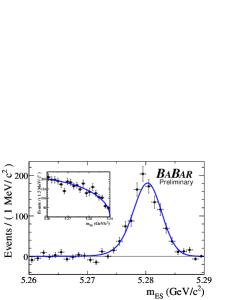
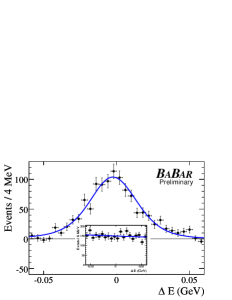
Figure 1: Distributions of kinematic variables (left) $m_{\rm ES}$ and (right) $\Delta E$ for the $K^{+}K^{-}{K^{0}_{\scriptscriptstyle S}}(\pi^{+}\pi^{-})$ sample. The plots show signal, with the continuum background shown in the insets. The points are data events weighted with the ${}_{s}{\cal P}lot$  technique, while the curves are the PDF shapes used in the ML fit (Sec. 4).

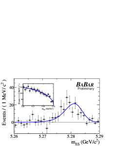
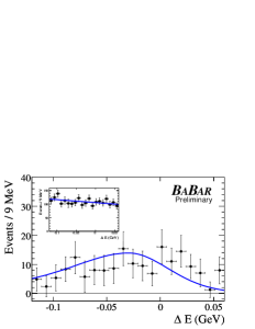
Figure 2: Distributions of kinematic variables (left) $m_{\rm ES}$ and (right) $\Delta E$ for the $K^{+}K^{-}{K^{0}_{\scriptscriptstyle S}}(\pi^{0}\pi^{0})$ sample. The plots show signal, with the continuum background shown in the insets. The points are data events weighted with the ${}_{s}{\cal P}lot$  technique, while the curves are the PDF shapes used in the ML fit (Sec. 4).

4 ANALYSIS OF THE DALITZ PLOT

Four-momentum conservation in a three-body decay gives the relation $M^{2}_{B^{0}}+m^{2}_{1}+m^{2}_{2}+m^{2}_{3}~{}=~{}m^{2}_{12}+m^{2}_{13}+m^{2}_{23}$, where $m^{2}_{ij}=(p_{i}+p_{j})^{2}$ is the square of the invariant mass of a daughter pair. This constraint leaves a choice of two independent Dalitz plot variables to describe the decay dynamics of a spin-zero particle. In this analysis we choose the $K^{+}K^{-}$ invariant mass $m_{K^{+}K^{-}}$ and the cosine of the helicity angle between the $K^{+}$ and the $K^{0}_{\scriptscriptstyle S}$ in the $K^{+}K^{-}$ center-of-mass frame, $\cos\theta_{H}$.

We perform an extended maximum likelihood fit to the measured time dependent Dalitz plot distribution. We first fit on the whole DP, then fit on the $m_{K^{+}K^{-}}>1.1{\mathrm{\,Ge\kern-1.00006ptV\!/}c^{2}}$ range (High-mass), then fit on the $m_{K^{+}K^{-}}<1.1{\mathrm{\,Ge\kern-1.00006ptV\!/}c^{2}}$ range (Low-mass). All fits are performed on the combined $K^{+}K^{-}{K^{0}_{\scriptscriptstyle S}}(\pi^{+}\pi^{-})$ and $K^{+}K^{-}{K^{0}_{\scriptscriptstyle S}}(\pi^{0}\pi^{0})$ samples simultaneously. The likelihood function ${\mathcal{L}}$ for each subsample is defined as

$${\mathcal{L}}=\exp{\left(-\sum_{i}n_{i}\right)}\prod_{j}\left[\sum_{i}n_{i}{\mathcal{P}}_{i,j}\right]$$ (1)

where $i$ labels the different signal and background components, $j$ runs over all events in the sample, and $n_{i}$ is the event yield for events of the $i$-th component. The probability density function (PDF) ${\mathcal{P}}_{i}$ of each component is defined as

$${\mathcal{P}}_{i}\equiv{\mathcal{P}}_{i}(\mbox{$m_{\rm ES}$})\cdot{\mathcal{P}}_{i}(\mbox{$\Delta E$})\cdot{\mathcal{P}}_{i}(\mathcal{F})\cdot{\mathcal{P}}_{DP,i}(m_{K^{+}K^{-}},\cos\theta_{H},{\rm\Delta}t,q_{tag})\otimes{\cal R}_{i}({\rm\Delta}t,\sigma_{{\rm\Delta}t}),$$ (2)

where $q_{tag}$ is the flavor of the tagged $B$ (1 for $B^{0}$ and -1 for $\kern 1.79993pt\overline{\kern-1.79993ptB}{}^{0}$), and ${\rm\Delta}t=t_{rec}-t_{tag}$ is the difference of the proper decay times of the two $B$-mesons in the $\mathchar 28935\relax{(4S)}$ decay. $\sigma_{{\rm\Delta}t}$ is the error on ${\rm\Delta}t$, and $\cal R$ is the ${\rm\Delta}t$ resolution function determined from a high statistics independent sample [5]. For the purpose of calculating the DP coordinates $m_{K^{+}K^{-}}$ and $\cos\theta_{H}$, we refit the $B$ candidates applying a $B$ mass constraint. This ensures that the $B$ candidates are reconstructed within the DP boundary. The Fisher discriminant PDF, ${\mathcal{P}}(\mathcal{F})$, is only used in the Low-mass fit (see Sec. 5). Because the Fisher discriminant is highly correlated with the position on the DP, we do not use the Fisher discriminant PDF for the fit to the whole DP or for the High-mass fit. The Fisher distributions are shown in Fig. 3. The PDFs for the individual fit components are described in more detail below.

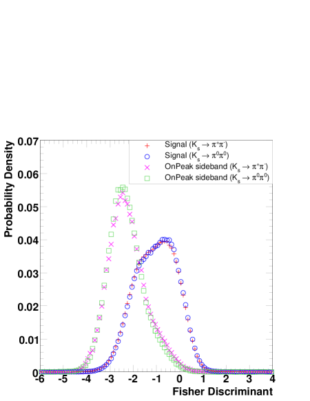
Figure 3: Fisher discriminant distributions for signal and continuum background and for $K^{+}K^{-}{K^{0}_{\scriptscriptstyle S}}(\pi^{+}\pi^{-})$ sample and $K^{+}K^{-}{K^{0}_{\scriptscriptstyle S}}(\pi^{0}\pi^{0})$ sample. Distributions are normalized to unit area.

4.1 Background in the Time-Dependent Dalitz Plot

We have two background components in our fit: continuum and $B\kern 1.79993pt\overline{\kern-1.79993ptB}{}$ background. For the continuum background component, we use the ARGUS function [19] for ${\mathcal{P}}(\mbox{$m_{\rm ES}$})$, and linear polynomial functions for ${\mathcal{P}}(\mbox{$\Delta E$})$. The ${\rm\Delta}t$ distribution is described by a double-Gaussian resolution function convolved with a PDF of the following form:

$${\cal P}({\rm\Delta}t)=f_{prompt}\delta({\rm\Delta}t)+(1-f_{prompt})e^{-|{\rm\Delta}t|/\tau_{bg}},$$ (3)

which allows for background decays with both zero and non-zero lifetimes. The Dalitz plot for the continuum background is parameterized using a two-dimensional histogram PDF in the variables $m_{K^{+}K^{-}}$ and $\cos\theta_{H}$. The histogram is filled with candidates from the region $5.2<\mbox{$m_{\rm ES}$}<5.26~{}{\mathrm{\,Ge\kern-1.00006ptV\!/}c^{2}}$.

We estimate the amount of $B\kern 1.79993pt\overline{\kern-1.79993ptB}{}$ background from Monte Carlo events. The $B\kern 1.79993pt\overline{\kern-1.79993ptB}{}$ background is almost purely combinatorial and is a few percent of the total background. In the $K^{+}K^{-}{K^{0}_{\scriptscriptstyle S}}(\pi^{+}\pi^{-})$ mode, the $m_{\rm ES}$ and $\Delta E$ PDFs for the $B\kern 1.79993pt\overline{\kern-1.79993ptB}{}$ backgrounds are parameterized with the same functional forms as the continuum backgrounds. Due to non-negligible correlation between $m_{\rm ES}$ and $\Delta E$ for $B\kern 1.79993pt\overline{\kern-1.79993ptB}{}$ background in the $K^{+}K^{-}{K^{0}_{\scriptscriptstyle S}}(\pi^{0}\pi^{0})$ mode, we construct a two-dimensional smoothed histogram PDF in those variables. The ${\rm\Delta}t$ distribution is described with a PDF similar to the continuum backgrounds, but we also allow for the possibility that the non-zero lifetime component has a time-dependent $C\!P$ asymmetry proportional to $\sin{\rm\Delta}m_{d}{\rm\Delta}t$ or $\cos{\rm\Delta}m_{d}{\rm\Delta}t$, where ${\rm\Delta}m_{d}$ is the mixing frequency of the $B^{0}$ meson. These asymmetries are set to zero in the nominal fit, but are varied as a systematic uncertainty. The Dalitz plot is described using a two-dimensional histogram PDF in a manner similar to the continuum backgrounds.

4.2 Signal Decays in the Time-Dependent Dalitz Plot

The signal components of the PDFs for ${\mathcal{P}}(\mbox{$m_{\rm ES}$})$ and ${\mathcal{P}}(\mbox{$\Delta E$})$ are parameterized using modified Gaussian distributions: ${\mathcal{P}}(x)\propto\exp[-(x-x_{0})^{2}/(2\sigma_{\pm}^{2}+\alpha_{\pm}(x-x_{0})^{2})].$ We determine the parameters $x_{0}$, $\sigma_{+}$, $\sigma_{-}$, $\alpha_{+}$, and $\alpha_{-}$ using MC events, and fix them in fits to data. For $x<x_{0}$ ($x>x_{0}$), the parameters $\sigma_{-},\alpha_{-}$ ($\sigma_{+},\alpha_{+}$) are used.

For signal events, the time-dependence is a function of location in the DP. When the flavor of the tagged $B$ $q_{tag}$, and the difference of the proper decay times ${\rm\Delta}t$, are measured, the time- and flavor-dependent decay rate over the Dalitz plot can be written as

$$d\Gamma=\frac{1}{(2\pi)^{3}}\frac{1}{32M_{B^{0}}^{3}}\frac{e^{-|{\rm\Delta}t|/\tau_{B^{0}}}}{4\tau_{B^{0}}} \times \Big{[}~{}\left|{\cal A}\right|^{2}+\left|\bar{{\cal A}}\right|^{2}+q_{tag}~{}(1-2w)~{}2Im\left(e^{-2i\cdot\beta}\bar{\cal A}{\cal A}^{*}\right)\sin{\rm\Delta}m_{d}{\rm\Delta}t$$ (4)

$$-~{}q_{tag}~{}(1-2w)~{}\left(\left|{\cal A}\right|^{2}-\left|\bar{{\cal A}}\right|^{2}\right)\cos{\rm\Delta}m_{d}{\rm\Delta}t~{}\Big{]},$$

where $q_{tag}=+1(-1)$ when the other $B$ meson is identified as a $B^{0}$ ($\kern 1.79993pt\overline{\kern-1.79993ptB}{}^{0}$) using a neural network technique [5]. The parameter $w$ is the fraction of events in which the $B$ meson is mistagged with the incorrect flavor, and the parameter $\beta$ is the CKM angle $\beta$, coming from $B^{0}$-$\kern 1.79993pt\overline{\kern-1.79993ptB}{}^{0}$ mixing. Approximately 75% of the signal events have tagging information and contribute to the measurement of CP violation parameters. After accounting for the mistag rate, the effective tagging efficiency is $(31.2\pm 0.3)\%$. Events without tagging information are assigned a mistag rate of $w=0.5$, and are included in the fit as they contribute to the determination of the Dalitz plot parameters. Decay amplitudes $\cal A$ and $\bar{\cal A}$ are defined in (6) and (7) below. $M_{B^{0}}$, $\tau_{B^{0}}$, and ${\rm\Delta}m_{d}$ are the mass, lifetime, and mixing frequency of the $B^{0}$ meson, respectively [1].

The PDF for the Dalitz plot rate takes the form

$${\cal P}_{DP}\propto d\Gamma(m_{K^{+}K^{-}},\cos\theta_{H},{\rm\Delta}t,q_{tag})\cdot\varepsilon(m_{K^{+}K^{-}},\cos\theta_{H})\cdot|J|\otimes{\cal R}({\rm\Delta}t,\sigma_{{\rm\Delta}t}),$$ (5)

where $|J(m_{K^{+}K^{-}})|=(2m_{K^{+}K^{-}})(2qp)$ is the Jacobian of the transformation $(m^{2}_{K^{+}K^{-}},m^{2}_{K^{+}K^{0}_{\scriptscriptstyle S}})\leftrightarrow(m_{K^{+}K^{-}},\cos\theta_{H})$, and is given in terms of the charged kaon momentum $q$ and neutral kaon momentum $p$, in the $K^{+}K^{-}$ frame. The efficiency $\varepsilon$ is calculated from high-statistics samples of simulated events and depends on the position on the Dalitz plot.

The amplitude $\cal A$ ($\bar{\cal A}$) for the decay $B^{0}\rightarrow K^{+}K^{-}K^{0}_{\scriptscriptstyle S}$ ($\kern 1.79993pt\overline{\kern-1.79993ptB}{}^{0}\rightarrow K^{-}K^{+}\overline{K^{0}_{\scriptscriptstyle S}}$) is, in our isobar model, written as a sum of decays through intermediate resonances:

$${\cal A} = \sum\limits_{r}c_{r}(1+b_{r})e^{i(\phi_{r}+\delta_{r})}\cdot f_{r},\hskip 28.45274pt\mathrm{and}$$ (6)

$$\bar{\cal A} = \sum\limits_{r}c_{r}(1-b_{r})e^{i(\phi_{r}-\delta_{r})}\cdot\bar{f}_{r}.$$ (7)

The isobar coefficients $c_{r}$ and $\phi_{r}$ are the magnitude and phase of the amplitude of component $r$, and we allow for different isobar coefficients for $B^{0}$ and $\kern 1.79993pt\overline{\kern-1.79993ptB}{}^{0}$ decays through the asymmetry parameters $b_{r}$ and $\delta_{r}$. The function $f_{r}=F_{r}\times T_{r}\times Z_{r}$ describes the dynamic properties of a resonance $r$, where $F_{r}$ is the form-factor for the resonance decay vertex, $T_{r}$ is the resonant mass-lineshape, and $Z_{r}$ describes the angular distribution in the decay [20, 21].

Our model includes the $\phi(1020)$, for which we use the Blatt-Weisskopf centrifugal barrier factor $F_{r}=1/\sqrt{1+(Rq)^{2}}$ [20], where $q$ is the daughter momentum in the resonance frame, and $R$ is the effective meson radius, taken to be $R=1.5~{}\mathrm{\,Ge\kern-1.00006ptV}^{-1}~{}(0.3~{}{\rm\,fm})$. For the scalar decays included in our model ($f_{0}(980)$, $X(1550)$, and $\chi_{c0}$), we use a constant form-factor. Note that we have omitted a similar centrifugal factor for the $B^{0}$ decay vertex into the $\phi K^{0}$ intermediate state since its effect is negligible due to the small width of the $\phi(1020)$ resonance.

The angular distribution is constant for scalar decays, whereas for vector decays $Z\sim\vec{q}\cdot\vec{p}$, where $\vec{q}$ is the momentum of the resonant daughter, and $\vec{p}$ is the momentum of the third particle in the resonance frame. We describe the line-shape for the $\phi(1020)$, $X(1550)$, and $\chi_{c0}$ using the relativistic Breit-Wigner function

$$T(m)=\frac{1}{m^{2}_{r}-m_{K^{+}K^{-}}^{2}-im_{r}\Gamma(m)},$$ (8)

where $m_{r}$ is the resonance pole mass. The mass-dependent width is given as $\Gamma(m_{K^{+}K^{-}})=\Gamma_{r}\left(q/q_{r}\right)^{2L+1}\left(m_{r}/m_{K^{+}K^{-}}\right)\left(F_{r}(q)/F_{r}(q_{r})\right)^{2},$ where $L$ is the resonance spin and $q=q_{r}$ when $m_{K^{+}K^{-}}=m_{r}$. For the $\phi(1020)$ and $\chi_{c0}$ parameters, we use average measurements [1]. The $X(1550)$ is less well-established. Previous Dalitz plot analyses of $B^{+}\rightarrow K^{+}K^{+}K^{-}$ [22, 24] and $B^{0}\rightarrow K^{+}K^{-}K^{0}$ decays [25] report observations of a scalar resonance at around 1.5 ${\mathrm{\,Ge\kern-1.00006ptV\!/}c^{2}}$. The scalar nature has been confirmed by partial-wave analyses [23, 24]. However, previous measurements report inconsistent resonant widths: $0.145\pm 0.029$ ${\mathrm{\,Ge\kern-1.00006ptV\!/}c^{2}}$ [22] and $0.257\pm 0.033$ ${\mathrm{\,Ge\kern-1.00006ptV\!/}c^{2}}$ [24]. Branching fractions also disagree, so the nature of this component is still unclear [26]. In our nominal fit, we take the resonance parameters from Ref. [24], which is based on a larger sample of $B\kern 1.79993pt\overline{\kern-1.79993ptB}{}$ decays than Ref. [22], and consider the narrower width given in the latter in the systematic error studies.

The $f_{0}(980)$ resonance is described with the coupled-channel (Flatté) function

$$T(m_{K^{+}K^{-}})=\frac{1}{m^{2}_{r}-m_{K^{+}K^{-}}^{2}-im_{r}(\rho_{K}g_{K}+\rho_{\pi}g_{\pi})},$$ (9)

where $\rho_{K}(m_{K^{+}K^{-}})=2\sqrt{1-4m^{2}_{K}/m_{K^{+}K^{-}}^{2}}$, $\rho_{\pi}(m_{K^{+}K^{-}})=2\sqrt{1-4m^{2}_{\pi}/m_{K^{+}K^{-}}^{2}}$, and the coupling strengths for the $KK$ and $\pi\pi$ channels are taken as $g_{\pi}=0.165\pm 0.018$ ${\mathrm{\,Ge\kern-1.00006ptV\!/}c^{2}}$, $g_{K}/g_{\pi}=4.21\pm 0.33$, and $m_{r}=0.965\pm 0.010$ ${\mathrm{\,Ge\kern-1.00006ptV\!/}c^{2}}$ [27].

In addition to resonant decays, we include non-resonant amplitudes. Existing models consider contributions from contact terms or higher-resonance tails [28, 29, 4], but they do not capture features observed in data. We rely on a phenomenological parameterization [22] and describe the non-resonant terms as

$${\cal A}_{NR}(\bar{\cal A}_{NR})=\left(c_{12}e^{i\phi_{12}}e^{-\alpha m^{2}_{12}}+c_{13}e^{i\phi_{13}}e^{-\alpha m^{2}_{13}}+c_{23}e^{i\phi_{23}}e^{-\alpha m^{2}_{23}}\right)\cdot(1\pm b_{NR})\cdot e^{\pm i\delta_{NR}},$$ (10)

where 1,2,3 denote the three daughter particles of the $B$ meson. The slope of the exponential function is consistent among previous measurements in both neutral and charged $B$ decays into three kaons [22, 24, 25], and we use $\alpha=0.14\pm 0.02~{}\mathrm{\,Ge\kern-1.00006ptV}^{-2}\cdot c^{4}$.

We compute the direct $C\!P$-asymmetry parameters for resonance $r$ from the asymmetries in amplitudes ($b_{r}$) and phases ($\delta_{r}$) given in Eqs. (6, 7). We define the rate asymmetry as

$${A}_{C\!P}(r)=\frac{|\bar{\cal A}_{r}|^{2}-|{\cal A}_{r}|^{2}}{|\bar{\cal A}_{r}|^{2}+|{\cal A}_{r}|^{2}}=\frac{-2b_{r}}{1+b_{r}^{2}},$$ (11)

and $\beta_{\mathit{eff}}(r)=\beta+\delta_{r}$ is defined as the total phase asymmetry. These asymmetries are related to the $C\!P$ asymmetry parameters $C$ and $-\eta S$ using the approximations

$$C_{r}\approx-{A}_{C\!P}(r),\hskip 28.45274pt\mathrm{and}$$ (12)

$$-\eta_{r}S_{r}\approx\frac{1-b_{r}^{2}}{1+b_{r}^{2}}\sin(2\beta_{\mathit{eff}}(r)),$$ (13)

where $\eta_{r}$ is the $C\!P$ eigenvalue of the final state. The fraction for resonance $r$ is computed as

$${\cal F}_{r}~{}=~{}\frac{\int d\cos\theta_{H}~{}dm_{K^{+}K^{-}}\cdot|J|\cdot(|{\cal A}_{r}|^{2}+|\bar{\cal A}_{r}|^{2})}{\int d\cos\theta_{H}~{}dm_{K^{+}K^{-}}\cdot|J|\cdot(|{\cal A}|^{2}+|\bar{\cal A}|^{2})}.$$ (14)

The sum of the fractions can be different from unity due to interference between the isobars.

In addition to the previously mentioned resonances, the decays $B^{0}\rightarrow D^{+}K^{-}~{}(D^{+}\rightarrow K^{+}K^{0}_{\scriptscriptstyle S})$ and $B^{0}\rightarrow D^{+}_{s}K^{-}~{}(D^{+}_{s}\rightarrow K^{+}K^{0}_{\scriptscriptstyle S})$ are also counted as signal. We include non-interfering amplitudes for these modes in our Dalitz plot model, parameterizing the $D_{(s)}$ mesons on the Dalitz plot as Gaussian distributions with widths taken from studies of simulated events. The parameters $b_{r}$ and $\delta_{r}$ are fixed to zero for the decays $B^{0}\rightarrow D^{+}K^{-}$, $B^{0}\rightarrow D^{+}_{s}K^{-}$, and $B^{0}\rightarrow\chi_{c0}K^{0}_{\scriptscriptstyle S}$ throughout this analysis.

5 RESULTS

In order to determine parameters of the Dalitz plot model, we perform three fits: 1) whole DP fit, 2) Low-mass ($m_{K^{+}K^{-}}<1.1{\mathrm{\,Ge\kern-1.00006ptV\!/}c^{2}}$) region fit, and 3) High-mass ($m_{K^{+}K^{-}}>1.1{\mathrm{\,Ge\kern-1.00006ptV\!/}c^{2}}$) region fit.

5.1 The whole Dalitz Plot fit

We perform a fit to both 4316 $B^{0}\rightarrow K^{+}K^{-}{K^{0}_{\scriptscriptstyle S}}(\pi^{+}\pi^{-})$ and 2205 $B^{0}\rightarrow K^{+}K^{-}{K^{0}_{\scriptscriptstyle S}}(\pi^{0}\pi^{0})$ candidates simultaneously in the full Dalitz plot. In this step we assume that all charmless decays have the same $C\!P$-asymmetry parameters. A Fisher discriminant cut ($-2.5<\mathcal{F}<4$), which retains about 95% of signal events and 60% of continuum events, is applied. We do not include the Fisher PDF in the fit. We vary the event yields, isobar coefficients, and the two $C\!P$-asymmetry parameters ${A}_{C\!P}$ and $\beta_{\mathit{eff}}$ averaged over the Dalitz plot. We find a signal yield of $1268\pm 43$ ($K^{+}K^{-}{K^{0}_{\scriptscriptstyle S}}(\pi^{+}\pi^{-})$) and $160\pm 19$ ($K^{+}K^{-}{K^{0}_{\scriptscriptstyle S}}(\pi^{0}\pi^{0})$) events, and a $B\kern 1.79993pt\overline{\kern-1.79993ptB}{}$ background yield of $47\pm 31$ ($K^{+}K^{-}{K^{0}_{\scriptscriptstyle S}}(\pi^{+}\pi^{-})$) and $24\pm 16$ ($K^{+}K^{-}{K^{0}_{\scriptscriptstyle S}}(\pi^{0}\pi^{0})$) events. The isobar amplitudes, phases, and fractions are listed in Table 1. The resonant fractions do not add up to 100% due to interference between the resonances. The $C\!P$-asymmetry parameters, and the correlation coefficients $\rho$ between them, are summarized in Table 2. Fig. 4 shows a projection of the Dalitz plot variable $m_{K^{+}K^{-}}$. Fig. 5 shows distributions of $\Delta t$ for $B^{0}$-tagged and $\kern 1.79993pt\overline{\kern-1.79993ptB}{}^{0}$-tagged events, and the asymmetry ${\cal A}(\Delta t)=(N_{B^{0}}-N_{\kern 1.25995pt\overline{\kern-1.25995ptB}{}^{0}})/(N_{B^{0}}+N_{\kern 1.25995pt\overline{\kern-1.25995ptB}{}^{0}})$, obtained with the ${}_{s}{\cal P}lot$ technique.

To calculate the significance of the nominal $\beta_{\mathit{eff}}$ result, many fits are performed with fixed but different $\beta_{\mathit{eff}}$ values. The change in likelihood as a function of $\beta_{\mathit{eff}}$ is shown in Fig. 6.

Decay		Amplitude $c_{r}$	Phase $\phi_{r}$	Fraction ${\cal F}_{r}$ (%)
$\phi(1020)K^{0}_{\scriptscriptstyle S}$		$0.00897\pm 0.00096$	$-0.341\pm 0.232$	$12.6\pm 1.0$
$f_{0}(980)K^{0}_{\scriptscriptstyle S}$		$0.542\pm 0.044$	$-0.201\pm 0.157$	$27.8\pm 7.1$
$X_{0}(1550)K^{0}_{\scriptscriptstyle S}$		$0.141\pm 0.017$	$-0.370\pm 0.154$	$5.70\pm 1.70$
$NR$	$(K^{+}K^{-})$	1 (fixed)	0 (fixed)	$98.1\pm 18.7$
	$(K^{+}K^{0}_{\scriptscriptstyle S})$	$0.328\pm 0.058$	$1.81\pm 0.23$	$10.5\pm 3.4$
	$(K^{-}K^{0}_{\scriptscriptstyle S})$	$0.353\pm 0.066$	$-1.44\pm 0.27$	$12.1\pm 3.8$
$\chi_{c0}K^{0}_{\scriptscriptstyle S}$		$0.0298\pm 0.0046$	$0.732\pm 0.437$	$2.53\pm 0.60$
$D^{+}K^{-}$		$1.34\pm 0.19$	–	$3.43\pm 0.69$
$D^{+}_{s}K^{-}$		$0.826\pm 0.160$	–	$1.37\pm 0.46$

Table 1: Isobar amplitudes and phases from the fit to the whole DP. Three rows for non-resonant (NR) contribution correspond to coefficients of exponential functions in Eq. (10). The errors are statistical only.

Name	Whole DP	High-mass
${A}_{C\!P}$	$0.03\pm 0.07\pm 0.02$	$0.05\pm 0.09\pm 0.04$
$\beta_{\mathit{eff}}$	$0.44\pm 0.07\pm 0.02$	$0.52\pm 0.08\pm 0.03$
$\rho$	$0.041$	$0.031$

Table 2: The $C\!P$-asymmetry parameters from the whole DP fit and the High-mass region fit. The first error is statistical and the second is systematic. $\rho$ is the correlation coefficient.

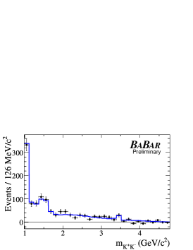
Figure 4: For the whole DP region fit, the distribution of the Dalitz plot variable $m_{K^{+}K^{-}}$ for signal-weighted data events (points) compared with the fit PDF in the $K^{+}K^{-}{K^{0}_{\scriptscriptstyle S}}(\pi^{+}\pi^{-})$ mode.

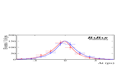
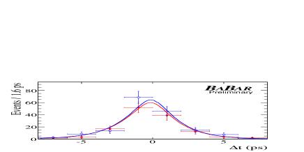
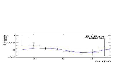
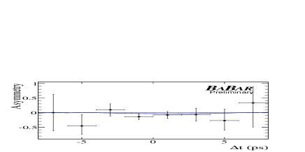
Figure 5: The ${\rm\Delta}t$ (top) distributions and asymmetries (bottom) in the whole DP (left) and Low-mass region (right), for the $K^{+}K^{-}{K^{0}_{\scriptscriptstyle S}}(\pi^{+}\pi^{-})$ mode. For the ${\rm\Delta}t$ distributions, $B^{0}$- ($\kern 1.79993pt\overline{\kern-1.79993ptB}{}^{0}$-) tagged signal-weighted events are shown as filled (open) circles, with the PDF projection in dashed red (solid blue).

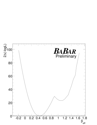
Figure 6: The change in the value of -2log($\mathcal{L}$) as a function of $\beta_{\mathit{eff}}$, for (a) the whole DP, (b) the High-mass region, (c) $f_{0}(980)$, and (d) $\phi(1020)$.

5.2 High-mass fit

We perform a fit to both 3112 $B^{0}\rightarrow K^{+}K^{-}{K^{0}_{\scriptscriptstyle S}}(\pi^{+}\pi^{-})$ and 1917 $B^{0}\rightarrow K^{+}K^{-}{K^{0}_{\scriptscriptstyle S}}(\pi^{0}\pi^{0})$ candidates in the High-mass region ($m_{K^{+}K^{-}}>1.1{\mathrm{\,Ge\kern-1.00006ptV\!/}c^{2}}$) simultaneously. We fix all isobar coefficients to the values from the whole DP fit. We vary yields and shared $C\!P$-asymmetry parameters. We find a signal yield of $894\pm 36$ $K^{+}K^{-}{K^{0}_{\scriptscriptstyle S}}(\pi^{+}\pi^{-})$ and $117\pm 16$ $K^{+}K^{-}{K^{0}_{\scriptscriptstyle S}}(\pi^{0}\pi^{0})$ events, and a $B\kern 1.79993pt\overline{\kern-1.79993ptB}{}$ background yield of $50\pm 31$ ($K^{+}K^{-}{K^{0}_{\scriptscriptstyle S}}(\pi^{+}\pi^{-})$) and $20\pm 15$ ($K^{+}K^{-}{K^{0}_{\scriptscriptstyle S}}(\pi^{0}\pi^{0})$) events. The fit results are summarized in Table 2. Fig. 7 shows a projection of the Dalitz plot variable $\cos\theta_{H}$ for events in this region, using the ${}_{s}{\cal P}lot$ technique.

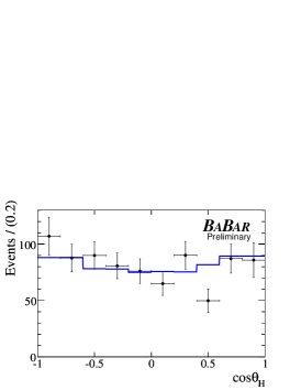
Figure 7: For the High-mass region fit, the distribution of the Dalitz plot variable $\cos\theta_{H}$ for signal-weighted data events (points) compared with the fit PDF in the $K^{+}K^{-}{K^{0}_{\scriptscriptstyle S}}(\pi^{+}\pi^{-})$ mode.

5.3 Low-mass fit

In order to measure $C\!P$-asymmetry parameters for components with low-$K^{+}\kern-1.60004ptK^{-}$ mass with reduced model-dependence from the rest of the DP, we select events using a cut of $m_{K^{+}K^{-}}<1.1{\mathrm{\,Ge\kern-1.00006ptV\!/}c^{2}}$. Because we are only selecting a small region of the DP, the correlation between the Fisher discriminant $\mathcal{F}$ and the DP location is unimportant. We therefore relax the cut on $\mathcal{F}$, and add the $\mathcal{F}$ PDF to the fit. After these requirements on $m_{K^{+}K^{-}}$ and $\mathcal{F}$, there are 1846 ($K^{+}K^{-}{K^{0}_{\scriptscriptstyle S}}(\pi^{+}\pi^{-})$) and 493 ($K^{+}K^{-}{K^{0}_{\scriptscriptstyle S}}(\pi^{0}\pi^{0})$) candidates remaining. The most significant contributions in this region come from $\phi(1020)$$K^{0}_{\scriptscriptstyle S}$ and $f_{0}(980)$$K^{0}_{\scriptscriptstyle S}$ decays, with a smaller contribution from a low-$K^{+}\kern-1.60004ptK^{-}$ mass tail of non-resonant decays. We fix all the isobar coefficients except for those of the $\phi(1020)$ to the values from the whole DP fit, and fix the $C\!P$-asymmetry parameters $b_{r}$ and $\delta_{r}$ for all resonances except the $\phi(1020)$ and $f_{0}(980)$ to be 0. We vary the events yields, isobar coefficients for the $\phi(1020)$, and separate $C\!P$-asymmetry parameters for the $\phi(1020)$ and $f_{0}(980)$ in the fit. We find signal yields of $381\pm 23$ ($K^{+}K^{-}{K^{0}_{\scriptscriptstyle S}}(\pi^{+}\pi^{-})$) and $40\pm 9$ ($K^{+}K^{-}{K^{0}_{\scriptscriptstyle S}}(\pi^{0}\pi^{0})$) events, and $B\kern 1.79993pt\overline{\kern-1.79993ptB}{}$ background yields of $12\pm 13$ ($K^{+}K^{-}{K^{0}_{\scriptscriptstyle S}}(\pi^{+}\pi^{-})$) and $-3\pm 5$ ($K^{+}K^{-}{K^{0}_{\scriptscriptstyle S}}(\pi^{0}\pi^{0})$) events

The $C\!P$-asymmetry results are listed in Table 3; the systematic uncertainties will be described in Sec. 6. We find two solutions with likelihood difference $\Delta$log($\mathcal{L}$) = 0.1. Solution (1) is consistent with the SM, while Solution (2) has a value of $\beta_{\mathit{eff}}$ for the $f_{0}(980)$$K^{0}_{\scriptscriptstyle S}$ decay that differs significantly from the SM, as shown in Table 3. The two solutions also have significantly different values of $c_{r}$ for the $\phi(1020)$. Both solutions also have a mathematical ambiguity of $\pm\pi$ radians on $\beta_{\mathit{eff}}$ for the $\phi(1020)$, and a correlated ambiguity of $\pm\pi$ radians on the isobar parameter $\phi_{r}$ for the $\phi(1020)$. This ambiguity is present because the decay amplitude contains interference terms that only depend on the linear combinations $\beta_{\mathit{eff}}+\phi_{r}$ and $\beta_{\mathit{eff}}-\phi_{r}$. We choose Solution (1) as our nominal solution. The correlation coefficients $\rho$ between the $C\!P$ parameters for Solution (1) are shown in Table 3. Because the decay rate depends on interference terms between the $\phi(1020)$$K^{0}_{\scriptscriptstyle S}$ and $f_{0}(980)$$K^{0}_{\scriptscriptstyle S}$ decays, the significant correlation between the measured $C\!P$ parameters is expected.

Name	Solution (1)	Solution (2)	Correlation
			1	2	3	4
1 ${A}_{C\!P}(\phi K^{0}_{\scriptscriptstyle S})$	$0.14\pm 0.19\pm 0.02$	$0.13\pm 0.18$	1.0	-0.09	-0.28	0.09
2 $\beta_{\mathit{eff}}(\phi K^{0}_{\scriptscriptstyle S})$	$0.13\pm 0.13\pm 0.02$	$0.14\pm 0.14$		1.0	0.54	0.65
3 ${A}_{C\!P}(f_{0}K^{0}_{\scriptscriptstyle S})$	$0.01\pm 0.26\pm 0.07$	$-0.49\pm 0.25$			1.0	0.25
4 $\beta_{\mathit{eff}}(f_{0}K^{0}_{\scriptscriptstyle S})$	$0.15\pm 0.13\pm 0.03$	$3.44\pm 0.19$				1.0

Table 3: $C\!P$-violation parameters for $B^{0}\rightarrow K^{+}K^{-}K^{0}_{\scriptscriptstyle S}$ for $m_{K^{+}K^{-}}<1.1~{}{\mathrm{\,Ge\kern-1.00006ptV\!/}c^{2}}$. The first error is statistical and the second is systematic. Correlation coefficients are given for Solution (1) only.

Fig. 8 shows projections of the Dalitz plot distributions of events in this region, using the ${}_{s}{\cal P}lot$ technique. Fig. 5 shows distributions of $\Delta t$ for $B^{0}$-tagged and $\kern 1.79993pt\overline{\kern-1.79993ptB}{}^{0}$-tagged events, and the asymmetry ${\cal A}(\Delta t)=(N_{B^{0}}-N_{\kern 1.25995pt\overline{\kern-1.25995ptB}{}^{0}})/(N_{B^{0}}+N_{\kern 1.25995pt\overline{\kern-1.25995ptB}{}^{0}})$.

The decay $B^{0}\rightarrow\phi(1020)K^{0}_{\scriptscriptstyle S}$, with highly suppressed tree amplitudes, is, in terms of theoretical uncertainty, the cleanest channel to interpret possible deviations of the $C\!P$-violation parameters from the SM expectations. Values of $\beta_{\mathit{eff}}$ are consistent with the value found in $[c\bar{c}]K^{0}$ decays [5, 6].

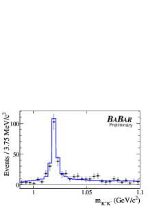
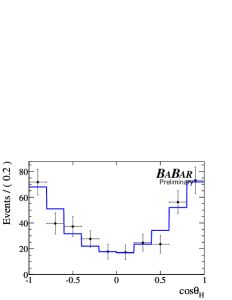
Figure 8: For the Low-mass region fit, the distributions of the Dalitz plot variables $m_{K^{+}K^{-}}$ (left) and $\cos\theta_{H}$ (right) for signal-weighted data events (points) compared with the fit PDF in the $K^{+}K^{-}{K^{0}_{\scriptscriptstyle S}}(\pi^{+}\pi^{-})$ mode.

We also calculate the parameters $C$ and $-\eta S$ for $\phi(1020)K^{0}_{\scriptscriptstyle S}$ and $f_{0}(980)K^{0}_{\scriptscriptstyle S}$ using the expressions in (12) and (13). The results are shown in Table 4, along with $C$ and $-\eta S$ for the whole DP and High-mass fits.

	$C$	$-\eta S$
Whole DP	$-0.03\pm 0.07\pm 0.02$	$0.77\pm 0.09\pm 0.02$
High-mass	$-0.05\pm 0.09\pm 0.04$	$0.86\pm 0.08\pm 0.03$
$\phi(1020)K^{0}_{\scriptscriptstyle S}$	$-0.14\pm 0.19\pm 0.02$	$0.26\pm 0.26\pm 0.03$
$f_{0}(980)K^{0}_{\scriptscriptstyle S}$	$-0.01\pm 0.26\pm 0.07$	$0.29\pm 0.25\pm 0.06$

Table 4: The $C\!P$ asymmetry parameters $C$ and $-\eta S$, derived using Equations (12) and (13). Results are shown for the whole DP, the High-mass region, and for both $\phi(1020)K^{0}_{\scriptscriptstyle S}$ and $f_{0}(980)K^{0}_{\scriptscriptstyle S}$ in the Low-mass region. For the Low-mass results, only Solution (1) is shown. The first error is statistical and the second is systematic.

6 SYSTEMATIC STUDIES

We study systematic effects on the $C\!P$-asymmetry parameters due to fixed parameters in the $m_{\rm ES}$ and $\Delta E$ PDFs. We assign systematic errors by comparing the fit with nominal parameters and with parameters varied by their error ($\pm 1\sigma$), and assign the average difference as the systematic error. In addition, we account for a potential fit bias using values observed in studies with MC samples generated with the nominal Dalitz plot model. We take the average values of the bias observed in these studies as the systematic error. We account for fixed ${\rm\Delta}t$ resolution parameters, $B^{0}$ lifetime, $B^{0}$-$\kern 1.79993pt\overline{\kern-1.79993ptB}{}^{0}$ mixing and flavor tagging parameters. We also assign an error due to interference between the CKM-suppressed $\bar{b}\rightarrow\bar{u}c\bar{d}$ and the favored $b\rightarrow c\bar{u}d$ amplitude for some tag-side $B$ decays [32]. Smaller errors due to beam-spot position uncertainty, detector alignment, and the boost correction are based on studies done in charmonium decays. In the cases of the Low-mass and High-mass fits, we also assign systematic errors due to the isobar coefficients that are fixed to the result from the whole DP fit. In all fits we assume no direct $C\!P$ violation in decays dominated by the $b\rightarrow c$ transition ($\chi_{c0}K^{0}_{\scriptscriptstyle S}$, $D_{(s)}K$).

We also assign an error due to uncertainty in the resonant and non-resonant line-shape parameters. The systematic uncertainty associated with the resonant component includes the uncertainty in the mass and width of the X(1550), estimated by replacing the parameters used in the nominal fit with the values found by different measurements: $m_{r}=1.491$ ${\mathrm{\,Ge\kern-1.00006ptV\!/}c^{2}}$, $\Gamma=0.145$ $\mathrm{\,Ge\kern-1.00006ptV}$ [22]. All the systematic uncertainties are summarized in Table. 5.

Parameter	Whole DP		$\phi K^{0}_{\scriptscriptstyle S}$		$f_{0}K^{0}_{\scriptscriptstyle S}$		High-mass
	${A}_{C\!P}$	$\beta_{\mathit{eff}}$	${A}_{C\!P}$	$\beta_{\mathit{eff}}$	${A}_{C\!P}$	$\beta_{\mathit{eff}}$	${A}_{C\!P}$	$\beta_{\mathit{eff}}$
Fixed PDF Parameters	0.010	0.010	0.014	0.010	0.025	0.015	0.013	0.010
Fit Bias	0.007	0.011	0.009	0.012	0.011	0.011	0.014	0.009
DCSD, Beam Spot, other	0.015	0.004	0.015	0.004	0.015	0.004	0.015	0.004
Dalitz Model	0.005	0.005	0.009	0.002	0.060	0.024	0.027	0.023
Total	0.020	0.016	0.024	0.016	0.068	0.031	0.036	0.026

Table 5: Summary of systematic errors on $C\!P$-asymmetry parameters. Errors for $\phi K^{0}_{\scriptscriptstyle S}$ and $f_{0}K^{0}_{\scriptscriptstyle S}$ $C\!P$-parameters are based on the Low-mass region fit. Total is obtained from the quadratic sum of the individual systematics.

7 CONCLUSIONS

We performed a ML fit to analyze the DP distribution of $B^{0}\rightarrow K^{+}K^{-}K^{0}_{\scriptscriptstyle S}$ decay with the full BABAR dataset. From a fit to the whole DP, we measure $\beta_{\mathit{eff}}=0.44\pm 0.07\pm 0.02$, ${A}_{C\!P}=0.03\pm 0.07\pm 0.02$, consistent with our previous measurements [15] and compatible with the Standard Model values $\beta\simeq 0.37,{A}_{C\!P}=0$. We measure $C\!P$ violation with a significance of 6.7 standard deviations (including statistical and systematic errors), and we reject the solution near $\pi/2-\beta$ at 4.8 standard deviations.

From a fit to the region of the DP with $m_{K^{+}K^{-}}>1.1{\mathrm{\,Ge\kern-1.00006ptV\!/}c^{2}}$, we measure $\beta_{\mathit{eff}}=0.52\pm 0.08\pm 0.03$ and ${A}_{C\!P}=0.05\pm 0.09\pm 0.04$, compatible with the Standard Model expectations. We measure $C\!P$ violation in this High-mass region at 6.7 standard deviations.

From a fit to events at low $K^{+}$ $K^{-}$ masses, we measure $\beta_{\mathit{eff}}=0.13\pm 0.13\pm 0.02$ and ${A}_{C\!P}=0.14\pm 0.19\pm 0.02$ for $B^{0}\rightarrow\phi(1020)K^{0}_{\scriptscriptstyle S}$, and $\beta_{\mathit{eff}}=0.15\pm 0.13\pm 0.03$ and ${A}_{C\!P}=0.01\pm 0.26\pm 0.07$ for $B^{0}\rightarrow f_{0}K^{0}_{\scriptscriptstyle S}$. The results for $\beta_{\mathit{eff}}$ are roughly 1.7 standard deviations below the Standard Model value.

These results supersede our previous measurements [15] made on a smaller dataset. All of our results are consistent with our previous measurements.

8 ACKNOWLEDGMENTS

We are grateful for the extraordinary contributions of our PEP-II colleagues in achieving the excellent luminosity and machine conditions that have made this work possible. The success of this project also relies critically on the expertise and dedication of the computing organizations that support BABAR. The collaborating institutions wish to thank SLAC for its support and the kind hospitality extended to them. This work is supported by the US Department of Energy and National Science Foundation, the Natural Sciences and Engineering Research Council (Canada), the Commissariat à l’Energie Atomique and Institut National de Physique Nucléaire et de Physique des Particules (France), the Bundesministerium für Bildung und Forschung and Deutsche Forschungsgemeinschaft (Germany), the Istituto Nazionale di Fisica Nucleare (Italy), the Foundation for Fundamental Research on Matter (The Netherlands), the Research Council of Norway, the Ministry of Education and Science of the Russian Federation, Ministerio de Educación y Ciencia (Spain), and the Science and Technology Facilities Council (United Kingdom). Individuals have received support from the Marie-Curie IEF program (European Union) and the A. P. Sloan Foundation.

References

- [1] W.-M. Yao et al. [Particle Data Group], J. Phys. G 33, 1 (2006)
- [2] M. Beneke, Phys. Lett. B 620, 143 (2005) [arXiv:hep-ph/0505075].
- [3] G. Buchalla, G. Hiller, Y. Nir and G. Raz, JHEP 0509, 074 (2005) [arXiv:hep-ph/0503151].
- [4] H. Y. Cheng, C. K. Chua and A. Soni, Phys. Rev. D 72, 094003 (2005) [arXiv:hep-ph/0506268].
- [5] B. Aubert et al. [BABAR Collaboration], Phys. Rev. Lett. 94, 161803 (2005) [arXiv:hep-ex/0408127].
- [6] K. Abe et al. [Belle Collaboration], [arXiv:hep-ex/0507037].
- [7] R. Itoh et al. [Belle Collaboration], Phys. Rev. Lett. 95, 091601 (2005)
- [8] P. Krokovny et al. [Belle Collaboration], Phys. Rev. Lett. 97, 081801 (2006)
- [9] J. Dalseno et al. [Belle Collaboration], Phys. Rev. D 76, 072004 (2007)
- [10] B. Aubert et al. [BABAR Collaboration], Phys. Rev. D 71, 032005 (2005) [arXiv:hep-ex/0411016].
- [11] B. Aubert et al. [BABAR Collaboration], Phys. Rev. D 74, 091101 (2006) [arXiv:hep-ex/0608016].
- [12] B. Aubert et al. [BABAR Collaboration], Phys. Rev. Lett. 99, 231802 (2007) [arXiv:0708.1544[hep-ex]].
- [13] J. Charles et al. (CKMfitter Group), Eur. Phys. J. C 41, 1-131 (2005) [arXiv:hep-ph/0406184], Updated results and plots available at: http://ckmfitter.in2p3.fr
- [14] M. Bona et al. (UTfit Collaboration), Phys. Rev. Lett. 97 151803 (2006), [arXiv:hep-ph/0605213], Updated results and plots available at: http://www.utfit.org
- [15] B. Aubert et al. [BABAR Collaboration], Phys. Rev. Lett. 99 161802 (2007) [arXiv:0706.3885[hep-ex]].
- [16] B. Aubert et al. [BABAR Collaboration], Nucl. Instrum. Meth. A 479, 1 (2002) [arXiv:hep-ex/0105044].
- [17] GEANT4 Collaboration, S. Agostinelli et al., Nucl. Instrum. Meth. A 506, 250 (2003)
- [18] M. Pivk and F. R. Le Diberder, Nucl. Instrum. Meth. A 555, 356 (2005) [arXiv:physics/0402083].
- [19] H. Albrecht et al. [ARGUS Collaboration], Z. Phys. C 48, 543 (1990).
- [20] J. M. Blatt, V. F. Weisskopf, “Theoretical Nuclear Physics”, John Wiley & Sons, New York (1952).
- [21] C. Zemach, Phys. Rev. 133, B1201 (1964).
- [22] A. Garmash et al. [BELLE Collaboration], Phys. Rev. D 71, 092003 (2005) [arXiv:hep-ex/0412066].
- [23] B. Aubert et al. [BABAR Collaboration], Phys. Rev. D 71, 091102 (2005) [arXiv:hep-ex/0502019].
- [24] B. Aubert et al. [BABAR Collaboration], [arXiv:hep-ex/0605003].
- [25] B. Aubert et al. [BABAR Collaboration], [arXiv:hep-ex/0507094].
- [26] P. Minkowski and W. Ochs, Eur. Phys. J. C 39, 71 (2005) [arXiv:hep-ph/0404194].
- [27] M. Ablikim et al. [BES Collaboration], Phys. Lett. B 607, 243 (2005) [arXiv:hep-ex/0411001].
- [28] H. Y. Cheng and K. C. Yang, Phys. Rev. D 66, 054015 (2002) [arXiv:hep-ph/0205133].
- [29] S. Fajfer, T. N. Pham and A. Prapotnik, Phys. Rev. D 70, 034033 (2004) [arXiv:hep-ph/0405065].
- [30] M. Gronau and J. L. Rosner, Phys. Rev. D 72, 094031 (2005) [arXiv:hep-ph/0509155].
- [31] B. Aubert et al. [BABAR Collaboration], Phys. Rev. D 72, 072003 (2005) [arXiv:hep-ex/0507004].
- [32] O. Long, M. Baak, R. Cahn, and D. Kirkby, Phys. Rev. D 68, 034010 (2003).