The BABAR Collaboration

1 INTRODUCTION

Weak decays of hadrons provide a straight access to the parameters of the CKM matrix and thus to the study of the $C\!P$ violation. Gluon scattering in the final state (Final State Interactions, or FSI) can modify the decay dynamics and so must be well understood. The two-body hadronic decays with a charmed final state, $B\rightarrow Dh$, are of great help in studying strong-interaction physics related with the confinement of quarks and gluons into hadrons.

The decays $B\rightarrow Dh$, where $h$ is a light meson, can proceed through the emission of a $W^{\pm}$ boson following three possible diagrams: external, internal (see Fig. 1) or by a $W^{\pm}$ boson exchange whose contribution is negligible [1].

Figure 1: External (a) and internal (b) tree diagrams for $\kern 1.79993pt\overline{\kern-1.79993ptB}{}^{0}\rightarrow Dh$ decays.

In the case of the decays $\kern 1.79993pt\overline{\kern-1.79993ptB}{}^{0}\rightarrow D^{(*)0}h^{0}$, the major contribution comes from the internal diagram [2]. Since mesons are color single objects, in internal diagrams $\kern 1.79993pt\overline{\kern-1.79993ptB}{}^{0}\rightarrow D^{(*)0}h^{0}$ the quarks from the $W^{\pm}$ decay are constrained to have the anti-color of the spectator quark, which induces a suppression of internal diagrams in comparison with external ones. Internal diagrams are so called color-suppressed and external ones are called color-favored.

In the factorization model  [2, 3, 4, 5], the non-factorizable interactions in the final state by soft gluons are neglected. The matrix element in the effective weak Hamiltonian of the decay $B\rightarrow Dh$ is then factorized into a product of asymptotic states. Factorization appears to be successful in the description of the color-favored decays [6].

The decays $\kern 1.79993pt\overline{\kern-1.79993ptB}{}^{0}\rightarrow D^{(*)0}\pi^{0}$ were first observed by CLEO [7] and Belle [8] with respectively 9.67 and 23.1$\times 10^{6}~{}B\kern 1.79993pt\overline{\kern-1.79993ptB}{}$ pairs. The Belle collaboration has also observed the decays $D^{0}\eta$ and $D^{0}\omega$ and put upper limits on the ${\cal BF}$ of $D^{*0}\eta$ and $D^{*0}\omega$ [8].

The branching fraction (${\cal BF}$) of the color-suppressed decays $\kern 1.79993pt\overline{\kern-1.79993ptB}{}^{0}\rightarrow D^{(*)0}\pi^{0}$, $D^{(*)0}\eta$, $D^{(*)0}\omega$, and $D^{0}\eta^{\prime}$ were measured recently by BABAR [9] with 88$\times 10^{6}~{}B\kern 1.79993pt\overline{\kern-1.79993ptB}{}$ pairs and an upper limit was set on the ${\cal BF}$ of $D^{*0}\eta^{\prime}$. The Belle collaboration measured with 152$\times 10^{6}~{}B\kern 1.79993pt\overline{\kern-1.79993ptB}{}$ pairs the ${\cal BF}$ of $\kern 1.79993pt\overline{\kern-1.79993ptB}{}^{0}\rightarrow D^{(*)0}h^{0}$, $h^{0}=\pi^{0}$, $\eta$, $\omega$, and $\eta^{\prime}$ [10, 11] and studied the decays $\kern 1.79993pt\overline{\kern-1.79993ptB}{}^{0}\rightarrow D^{(*)0}\rho^{0}$ with 388$\times 10^{6}~{}B\kern 1.79993pt\overline{\kern-1.79993ptB}{}$ pairs [12]. Many of these measurements showed a significant disagreement with predictions by factorization [13], but stronger experimental constraints are needed to distinguish between the different models of the color-suppressed dynamics like pQCD (perturbative QCD) [14, 15] or SCET (Soft Collinear Effective Theory) [16, 17, 18]. This paper reports the branching fraction measurement of eight color-suppressed decays $\kern 1.79993pt\overline{\kern-1.79993ptB}{}^{0}\rightarrow D^{(*)0}\pi^{0}$, $D^{(*)0}\eta$, $D^{(*)0}\omega$ and $D^{(*)0}\eta^{\prime}$ with 454$\times 10^{6}~{}B\kern 1.79993pt\overline{\kern-1.79993ptB}{}$ pairs.

2 THE BABAR DETECTOR AND DATASET

The data used in this analysis were collected with the BABAR detector at the PEP-II asymmetric $e^{+}e^{-}$ storage ring. The BABAR detector is described in detail in Ref. [19]. Charged particle tracks are reconstructed using a five-layer silicon vertex tracker (SVT) and a 40-layer drift chamber (DCH) immersed in a 1.5 T magnetic field. Tracks are identified as pions or kaons (particle identification or PID) based on likelihoods constructed from energy loss measurements in the SVT and the DCH and from Cherenkov radiation angles measured in the detector of Cherenkov light (DIRC). Photons are reconstructed from showers measured in the electromagnetic calorimeter (EMC). Muon and neutral hadron identification are performed with the instrumented flux return (IFR).

The data sample consists of an integrated luminosity of 413 $\mbox{\,fb}^{-1}$ recorded at the $\mathchar 28935\relax(4S)$ resonance with a center-of-mass (CM) energy of 10.58 $\mathrm{\,Ge\kern-1.00006ptV}$, corresponding to $(454\pm 5)\times 10^{6}~{}B\kern 1.79993pt\overline{\kern-1.79993ptB}{}$ pairs. A data sample of 41 $\mbox{\,fb}^{-1}$ with a CM energy 40 $\mathrm{\,Me\kern-1.00006ptV}$ below the $\mathchar 28935\relax(4S)$ resonance is used to study background contributions from continuum events $e^{+}e^{-}\rightarrow q\overline{q}$ ($q=u$, $d$, $s$, $c$).

Samples of simulated Monte Carlo (MC) events were used to determine signal and background characteristics, optimize selection criteria and evaluate efficiencies. Simulated events $e^{+}e^{-}\rightarrow\mathchar 28935\relax(4S)\rightarrow B^{+}{\kern-1.60004ptB^{-}},~{}B^{0}\kern 1.79993pt\overline{\kern-1.79993ptB}{}^{0}$, $e^{+}e^{-}\rightarrow q\overline{q}$ ($q=u$, $d$, $s$) and $e^{+}e^{-}\rightarrow c\overline{c}$ are generated with EvtGen [20], which interfaces to Pythia [21] and Jetset [22]. Separate samples of exclusive $\kern 1.79993pt\overline{\kern-1.79993ptB}{}^{0}\rightarrow D^{(*)0}h^{0}$ decays were generated to evaluate the signal features and the efficiency of selections on signal. A sample of exclusive $B^{-}\rightarrow D^{(*)0}\rho^{-}$ was generated for the study of that background. All MC samples include simulation of the BABAR detector response generated through GEANT4 [23]. The integrated luminosity of the MC samples is about three times the data luminosity for $B\kern 1.79993pt\overline{\kern-1.79993ptB}{}$, one times the data luminosity for $e^{+}e^{-}\rightarrow q\overline{q}$ ($q=u$, $d$, $s$) and two times for $e^{+}e^{-}\rightarrow c\overline{c}$. The equivalent integrated luminosities of the exclusive simulations range from 50 to 2500 times the data luminosity.

3 ANALYSIS METHOD

3.1 Event reconstruction

Charged particles tracks are reconstructed from measurements in the SVT and$/$or the DCH, and an identification is assigned by the PID algorithm. Extrapolated tracks must be in the vicinity of the $e^{+}e^{-}$ interaction point, $i.e.$ within 1.5 cm in the plane transverse to the beam axis and 2.5 cm along the beam axis. The tracks used for the reconstruction of $\eta\rightarrow\pi^{+}\pi^{-}\pi^{0}$ must in addition have a transverse momentum $p_{T}$ larger than 50 ${\mathrm{\,Me\kern-1.00006ptV\!/}c}$. When PID criterion is required on a track, the track polar angle $\theta$ must be in the DIRC fiducial region $25.78^{\circ}<\theta<146.10^{\circ}$. Photons are defined as single bumps in the EMC crystals not matched with any track, and with a shower lateral shape consistent with a photon. Because of high background in the forward region of the EMC caused by the beam asymmetry, the photons detected in the region $\theta<21.19^{\circ}$ are rejected.

Intermediate resonances of the decays $\kern 1.79993pt\overline{\kern-1.79993ptB}{}^{0}\rightarrow D^{(*)0}h^{0}$ are reconstructed by combining tracks and$/$or photons for the channels with the highest decay rate and detection efficiency. When mesons are combined to build a resonance, masses are fixed to their nominal value [24]. For the $\omega$ and $\rho^{0}$ mesons, whose natural width is not negligible in comparison with the experimental resolution, their mass is not fixed to the nominal value. The selections applied to each meson $\pi^{0}$, $\eta$, $\omega$, $\eta^{\prime}$, $D^{0}$, and $D^{*0}$ are optimized by maximizing the figure of merit $S/\sqrt{S+B}$ where $S$ is the number of signal and $B$ is the number of background events. The numbers $S$ and $B$ are computed from simulations, the ${\cal BF}$’s used to evaluate $S$ are the world average value given by PDG [24]. Each resonance mass distribution is fitted with a set of Gaussian functions or a modified Novosibirsk function [29], which is composed of a Gaussian-like peaking part with two tails at low and high values. Resonance candidates are then required to have a mass within $\pm 2.5~{}\sigma$ around the fitted mass central value, where $\sigma$ is the resolution of the mass distribution obtained by the fit. For the resonances $D^{0}\rightarrow K^{-}\pi^{+}\pi^{0}$ and $D^{*0}\rightarrow D^{0}\gamma$, the lower bound is extended to $-3\sigma$ because of the photon energy losses in front and between the EMC crystals, which makes the mass distribution asymmetric with a tail at low values.

3.2 Selection of intermediate resonances

3.2.1 $\pi^{0}$ selection

The $\pi^{0}$ mesons are reconstructed by combining two photons, each photon energy $E(\gamma)$ must be larger than 85 $\mathrm{\,Me\kern-1.00006ptV}$ for $\pi^{0}$ coming from $B^{0}$ decay, and larger than 60 $\mathrm{\,Me\kern-1.00006ptV}$ for $\pi^{0}$ coming from $\eta$, $\omega$ or $D^{0}$. Soft $\pi^{0}$’s coming from $D^{*0}\rightarrow D^{0}\pi^{0}$ must satisfy $E(\gamma)>30~{}\mathrm{\,Me\kern-1.00006ptV}$. The reconstruction resolution for high momentum $\pi^{0}$ is limited by the angle between the two daughter photons; for low momentum $\pi^{0}$ the resolution is limited by the neutral hadron background in EMC. The $\pi^{0}$ reconstructed mass resolution is about $6~{}{\mathrm{\,Me\kern-1.00006ptV\!/}c^{2}}$ for $\pi^{0}$ coming from $\eta$, $7~{}{\mathrm{\,Me\kern-1.00006ptV\!/}c^{2}}$ for $\pi^{0}$ coming from $\omega$ or $D^{0}$, and $8~{}{\mathrm{\,Me\kern-1.00006ptV\!/}c^{2}}$ for $\pi^{0}$ coming from $B^{0}$ or $D^{*0}$. The selection efficiency on signal ranges from 85 to 93 $\%$.

3.2.2 $\eta$ selection

The $\eta$ mesons are reconstructed in the $\gamma\gamma$ and $\pi^{+}\pi^{-}\pi^{0}$ decay modes. These modes account for 62 $\%$ of the total decay rate [24], and may originate from $\kern 1.79993pt\overline{\kern-1.79993ptB}{}^{0}\rightarrow D^{(*)0}\eta$ or $\eta^{\prime}\rightarrow\pi^{+}\pi^{-}\eta$ decays.

The $\eta\rightarrow\gamma\gamma$ candidates are reconstructed by combining two photons that satisfy $E(\gamma)>200~{}\mathrm{\,Me\kern-1.00006ptV}$ for $\kern 1.79993pt\overline{\kern-1.79993ptB}{}^{0}$ daughters and $E(\gamma)>180~{}\mathrm{\,Me\kern-1.00006ptV}$ for $\eta^{\prime}$ daughters. As high momentum $\pi^{0}$s may fake $\eta\rightarrow\gamma\gamma$ decays, a veto is applied against $\pi^{0}$: for each $\eta\rightarrow\gamma_{1}\gamma_{2}$ candidate, the photons $\gamma_{1/2}$ are associated with photons of the rest of event $\gamma_{i}$. If $E(\gamma_{i})>200~{}\mathrm{\,Me\kern-1.00006ptV}$ and the invariant mass of the pair $\{\gamma_{1}\gamma_{i}\}$ or $\{\gamma_{2}\gamma_{i}\}$ is in the $\pi^{0}$ mass window $115<m(\gamma_{1/2}\gamma_{i})<150~{}{\mathrm{\,Me\kern-1.00006ptV\!/}c^{2}}$, then the $\eta$ candidate is rejected. The resolution of the $\eta\rightarrow\gamma\gamma$ mass distribution is dominated by the EMC resolution and is about $15~{}{\mathrm{\,Me\kern-1.00006ptV\!/}c^{2}}$.

For $\eta$ candidates reconstructed in $\pi^{+}\pi^{-}\pi^{0}$, the $\pi^{0}$ is required to satisfy the conditions described in Section 3.2.1. The mass resolution is about $3.5~{}{\mathrm{\,Me\kern-1.00006ptV\!/}c^{2}}$, which is smaller than for $\eta\rightarrow\gamma\gamma$ thanks to the higher resolution of the tracking system. The selection efficiency on signal is about 77 $\%$ for $\eta\rightarrow\gamma\gamma$ and 75 $\%$ for $\eta\rightarrow\pi^{+}\pi^{-}\pi^{0}$.

3.2.3 $\omega$ selection

The $\omega$ mesons are reconstructed in the $\pi^{+}\pi^{-}\pi^{0}$ decay mode. These modes account for 89 $\%$ of the total decay rate. The $\pi^{0}$s are required to satisfy the conditions described in Section 3.2.1 and the $\pi^{\pm}$ must fulfill the condition $p_{T}(\pi^{\pm})>200~{}{\mathrm{\,Me\kern-1.00006ptV\!/}c}$. The natural width of the $\omega$ mass distribution $\Gamma\sim 8.49~{}\mathrm{\,Me\kern-1.00006ptV}$ [24] is comparable to the experimental resolution $\sigma\sim 7~{}{\mathrm{\,Me\kern-1.00006ptV\!/}c^{2}}$, therefore the $\omega$ mass is not constrained to its nominal value. We define a total width $\sigma_{tot}=\sqrt{\sigma^{2}+\Gamma^{2}}\sim 11~{}{\mathrm{\,Me\kern-1.00006ptV\!/}c^{2}}$ and require the $\omega$ candidates to satisfy $|m(\omega)-m(\omega)_{\textrm{mean}}|<2.5~{}\sigma_{tot}$. The selection efficiency on signal is about 82 $\%$.

3.2.4 $\rho^{0}$ selection

The $\rho^{0}$ mesons originate from $\eta^{\prime}\rightarrow\rho^{0}\gamma$ and are reconstructed in the $\pi^{+}\pi^{-}$ decay mode. These modes account for 100 $\%$ of the total decay rate. Charged particle tracks must satisfy $p_{T}(\pi^{\pm})>100~{}{\mathrm{\,Me\kern-1.00006ptV\!/}c}$. We define the helicity angle $\theta_{\rho^{0}}$ as the angle between the pion momentum in the $\rho^{0}$ rest frame and the $\rho^{0}$ momentum in the $\eta^{\prime}$ rest frame. Because the $\rho^{0}$ is a vector and pion is a pseudoscalar, the angular distribution is proportional to $\sin(\theta_{\rho^{0}})^{2}$ for pure signal and is flat for background. The $\rho^{0}$ candidates with $|\cos(\theta_{\rho^{0}})|>0.73$ are rejected. Due to the $\rho^{0}$ large natural width $\Gamma\sim 149.4~{}\mathrm{\,Me\kern-1.00006ptV}$ [24], no mass constraint is applied to the $\rho^{0}$. The mass of the $\rho^{0}$ candidates must be within 160 ${\mathrm{\,Me\kern-1.00006ptV\!/}c^{2}}$ around the nominal mass value.

3.2.5 $\eta^{\prime}$ selection

The $\eta^{\prime}$ mesons are reconstructed in the $\pi^{+}\pi^{-}\eta(\rightarrow\gamma\gamma)$ and $\rho^{0}\gamma$ decay modes. These modes account for 30 $\%$ of the total decay rate. For the reconstruction of $\eta^{\prime}\rightarrow\pi^{+}\pi^{-}\eta(\rightarrow\gamma\gamma)$, the $\eta$ candidates must satisfy the selections described in Section 3.2.2. The $\eta^{\prime}$ mass resolution is about $3~{}{\mathrm{\,Me\kern-1.00006ptV\!/}c^{2}}$.

For $\eta^{\prime}$ candidates reconstructed in $\rho^{0}\gamma$, the $\rho^{0}$’s are required to satisfy the conditions described in Section 3.2.4 and the photons must have an energy larger than 200 $\mathrm{\,Me\kern-1.00006ptV}$. As photons coming from $\pi^{0}$ decays may fake signal, the veto against $\pi^{0}$ described in Section 3.2.2 is applied. The $\eta^{\prime}$ mass resolution is about 8 ${\mathrm{\,Me\kern-1.00006ptV\!/}c^{2}}$, which is worse than $\eta^{\prime}\rightarrow\pi^{+}\pi^{-}\eta$ because of the resolution on gamma reconstruction and the large $\rho$ mass width.

The selection efficiency on signal is about 69 $\%$ for $\eta^{\prime}\rightarrow\pi^{+}\pi^{-}\eta(\rightarrow\gamma\gamma)$ and 66 $\%$ for $\eta^{\prime}\rightarrow\rho^{0}\gamma$.

3.2.6 $K^{0}_{\scriptscriptstyle S}$ selection

The $K^{0}_{\scriptscriptstyle S}$ mesons are reconstructed in the $\pi^{-}\pi^{+}$ decay modes. These modes account for 69 $\%$ of the total decay rate. The $\chi^{2}$ probability of the vertex fit of charged pions must be larger than 0.1 $\%$. We define the flight significance as the ratio $L/\sigma_{L}$ where $L$ is the $K^{0}_{\scriptscriptstyle S}$ flight length in the plane transverse to the beam axis and $\sigma_{L}$ is the uncertainty on $L$ determined from the vertex fit constraint. The combinatorial background is rejected by requiring a flight significance larger than 5. The reconstructed $K^{0}_{\scriptscriptstyle S}$ mass resolution is about 2 ${\mathrm{\,Me\kern-1.00006ptV\!/}c^{2}}$. The selection efficiency on signal is about 86 $\%$.

3.2.7 $D^{0}$ selection

The $D^{0}$ mesons are reconstructed in $K^{-}\pi^{+}$, $K^{-}\pi^{+}\pi^{0}$, $K^{-}\pi^{+}\pi^{-}\pi^{+}$, and $K^{0}_{\scriptscriptstyle S}\pi^{+}\pi^{-}$ decay modes. These modes account for about 28 $\%$ of the total decay rate. All $D^{0}$ candidates must satisfy $p^{*}(D^{0})>1.1~{}{\mathrm{\,Ge\kern-1.00006ptV\!/}c}$. That requirement is loose enough that background populate the sidebands of the signal region. The $\pi^{\pm}$’s coming from the $D^{0}$ candidate must fulfill $p_{T}(\pi^{\pm})>400~{}{\mathrm{\,Me\kern-1.00006ptV\!/}c}$ for $D^{0}\rightarrow K^{-}\pi^{+}$, $p_{T}(\pi^{\pm})>100~{}{\mathrm{\,Me\kern-1.00006ptV\!/}c}$ for $D^{0}\rightarrow K^{-}\pi^{+}\pi^{-}\pi^{+}$ and $p_{T}(\pi^{\pm})>120~{}{\mathrm{\,Me\kern-1.00006ptV\!/}c}$ for $D^{0}\rightarrow K^{0}_{\scriptscriptstyle S}\pi^{-}\pi^{+}$. The $\chi^{2}$ probability of the vertex fit of charged pions must be larger than 0.1 $\%$ for $D^{0}\rightarrow K^{-}\pi^{+}$ and larger than 0.5 $\%$ for the other modes. The kaon candidates must satisfy tight kaon criteria for $K^{-}\pi^{+}$ and $K^{-}\pi^{+}\pi^{0}$, and a loose kaon criteria for $K^{-}\pi^{+}\pi^{-}\pi^{+}$. For $K^{0}_{\scriptscriptstyle S}\pi^{+}\pi^{-}$, the $K^{0}_{\scriptscriptstyle S}$ candidates must satisfy the selection criteria described in Section 3.2.6.

The decay $D^{0}$ to $K^{-}\pi^{+}\pi^{0}$ proceeds mainly through the resonances $K^{*}$ ($K^{*0}\rightarrow K^{-}\pi^{+}$ or $K^{*-}\rightarrow K^{-}\pi^{0}$) and $\rho^{+}(\pi^{+}\pi^{0})$. Combinatorial background is rejected by using the parametrization of the $K^{-}\pi^{+}\pi^{0}$ Dalitz distribution studied by the Fermilab E691 experiment [25]. The $D^{0}$ candidates that are not in the resonance regions of the Dalitz distribution are rejected. The $\pi^{0}$ must satisfy the selections described in Section 3.2.1.

The reconstructed $D^{0}$ mass resolution is about 4, 5, 6, and 11 ${\mathrm{\,Me\kern-1.00006ptV\!/}c^{2}}$ for $K^{-}\pi^{+}\pi^{-}\pi^{+}$, $K^{0}_{\scriptscriptstyle S}\pi^{+}\pi^{-}$, $K^{-}\pi^{+}$, and $K^{-}\pi^{+}\pi^{0}$ modes, respectively. To account for the asymmetry in the mass distribution of $D^{0}\rightarrow K^{-}\pi^{+}\pi^{0}$, we require that the $D^{0}$ candidates satisfy $-3~{}\sigma<(m(D^{0})-m(D^{0})_{\textrm{mean}})<2.5~{}\sigma$.

The selection efficiency on signal is about 71 $\%$ for $K^{-}\pi^{+}$, 60 $\%$ for $K^{-}\pi^{+}\pi^{-}\pi^{+}$, 71 $\%$ for $K^{0}_{\scriptscriptstyle S}\pi^{+}\pi^{-}$, and 44 $\%$ for $K^{-}\pi^{+}\pi^{0}$.

3.2.8 $D^{*0}$ selection

The $D^{*0}$ mesons are reconstructed in the $D^{0}\pi^{0}$ and $D^{0}\gamma$ decay modes. The $\pi^{0}$ and $D^{0}$ candidates are required to satisfy the selections described in Section 3.2.1 and 3.2.7 respectively. The photons from $D^{*0}\rightarrow D^{0}\gamma$ must fulfill $E(\gamma)>200~{}\mathrm{\,Me\kern-1.00006ptV}$ and pass the veto against $\pi^{0}$ described in Section 3.2.2.

The resolution of the mass difference $\Delta m\equiv m(D^{*0})-m(D^{0})$ is about 2 ${\mathrm{\,Me\kern-1.00006ptV\!/}c^{2}}$ for $D^{0}\pi^{0}$ and 7 ${\mathrm{\,Me\kern-1.00006ptV\!/}c^{2}}$ for $D^{0}\gamma$. The $D^{*0}\rightarrow D^{0}\pi^{0}$ candidates must satisfy $|\Delta m-\Delta m_{\textrm{mean}}|<2.5~{}\sigma$. Because of the asymmetry of the $\Delta m$ distribution for $D^{0}\gamma$, the $D^{*0}$ candidates must satisfy $-3~{}\sigma<(\Delta m-\Delta m_{\textrm{mean}})<2.5~{}\sigma$.

The selection efficiency on signal is about 49 $\%$ for $D^{0}\pi^{0}$ and 39 $\%$ for $D^{0}\gamma$.

3.3 Selection of $B$ candidates

The $B$ candidates are reconstructed by combining a $D^{(*)0}$ with an $h^{0}$, with the $D^{*0}$ and $h^{0}$ masses constrained to their nominal value except when $h^{0}$ is the $\omega$. One needs to discriminate real $B$’s from fake ones created from combinatorial or crossfeed background.

3.3.1 $B$ kinematic variables

Two kinematic variables are used in BABAR to select $B$ candidates: the energy-substituted mass $m_{\rm ES}$ and the energy difference $\Delta E$. These two variables use the constraints from the precise knowledge of the beams’ energies and from energy conservation in the two-body decay $\mathchar 28935\relax(4S)\rightarrow B\kern 1.79993pt\overline{\kern-1.79993ptB}{}$. The quantity $m_{\rm ES}$ is the invariant mass of the $B$ candidate where the $B$ energy is set to the beam energy in the CM frame:

$$\mbox{$m_{\rm ES}$}=\sqrt{\left(\frac{\sqrt{s}}{2}\right)^{2}-|\overrightarrow{p^{*}_{B}}|^{2}},$$ (1)

and $\Delta E$ is the energy difference between the reconstructed $B$ energy and the beam energy in the CM frame:

$$\mbox{$\Delta E$}=E^{*}_{B}-\sqrt{s}/2,$$ (2)

where $\sqrt{s}$ is the $e^{+}e^{-}$ CM energy and $(E^{*}_{B},\overrightarrow{p_{B}})$ is the $B$ quadrivector in the CM frame. For $B$ signal events, the $m_{\rm ES}$ distribution peaks at the $B$ mass with a resolution of about 3 ${\mathrm{\,Me\kern-1.00006ptV\!/}c^{2}}$ dominated by the beam energy spread, whereas $\Delta E$ peaks near zero with a resolution of $15-50~{}\mathrm{\,Me\kern-1.00006ptV}$ depending on the number of photons in the final state.

3.3.2 Rejection of $e^{+}e^{-}\rightarrow q\overline{q}$ background

The continuum background $e^{+}e^{-}\rightarrow q\overline{q}$ ($q=u$, $d$, $s$ or mainly $c$) creates real high momentum mesons $D^{(*)0}$, $\pi^{0}$, $\eta^{(^{\prime})}$, $\omega$ that can fake the signal mesons originating from the two body decays $\kern 1.79993pt\overline{\kern-1.79993ptB}{}^{0}\rightarrow D^{(*)0}h^{0}$. That background is thus not rejected by the selections on intermediate resonances. Since the $B$ mesons are produced almost at rest in the $\mathchar 28935\relax(4S)$ frame, so the $\mathchar 28935\relax(4S)\rightarrow B\kern 1.79993pt\overline{\kern-1.79993ptB}{}$ events shape is spherical. By comparison, the $q\overline{q}$ events have a back-to-back jet-like shape given that the quark masses ($q\neq b$) are small compared to the CM energy. The $q\overline{q}$ background can hence be discriminated by the event shape described by the following variables:

• The thrust angle $\theta_{T}$ defined as the angle between the thrust axis of the $B$ candidate and the thrust axis of the rest of event. The thrust axis $\widehat{T}$ is defined as the axis that maximizes the quantity $T$:

  $$T=\frac{\sum_{i}|\overrightarrow{p_{i}}\cdot\widehat{T}|}{\sum_{i}|\overrightarrow{p_{i}}|}.$$ (3)

  The distribution of $|\cos(\theta_{T})|$ is flat for signal and peaks at $1$ for continuum background.

• Legendre monomials $L_{0}$ and $L_{2}$ defined as:

  $$L_{0}=\sum_{i}p^{*}_{i}\ ;\ L_{2}=\sum_{i}p^{*}_{i}|\cos(\theta^{*}_{i})|^{2},$$ (4)

  with $p_{i}^{*}$ the momentum of the particle $i$ that does not come from a $B$ candidate, and $\theta_{i}^{*}$ is the angle between $p_{i}^{*}$ and the thrust axis of the $B$ candidate.

• The polar angle $\theta^{*}_{B}$ between the $B$ momentum in the $\mathchar 28935\relax(4S)$ frame and the beam axis. The $\mathchar 28935\relax(4S)$ being vector ($J=1$) and the $B$ mesons being pseudoscalar ($J=0$), the angular distribution is proportional to $\sin^{2}(\theta^{*}_{B})$ for signal and roughly flat for background.

These four variables are combined in a Fisher discriminant built with the $T$MVA [26] toolkit package. The Fisher $\mathcal{F}_{shape}$ is trained with signal MC events and off-peak data events; in order to maximize the number of off-peak events all the $\kern 1.79993pt\overline{\kern-1.79993ptB}{}^{0}\rightarrow D^{(*)0}h^{0}$ modes are combined. The training and test are performed with $2\times 20000$ signal events and $2\times 20000$ off-peak events. The obtained Fisher formula is:

$$\mathcal{F}_{shape}=2.36-1.18\cdot|\cos(\theta_{T})|+$$

$$0.20\cdot L_{0}-1.01\cdot L_{2}-0.80\cdot|\cos(\theta_{B}^{*})|.$$ (5)

The $q\overline{q}$ background is rejected by applying a selection on $\mathcal{F}_{shape}$. The selection is optimized for each $\kern 1.79993pt\overline{\kern-1.79993ptB}{}^{0}$ signal mode by maximizing the statistical significance with signal MC against generic MC $e^{+}e^{-}\rightarrow q\overline{q}$, $q\neq b$. That requirement retains between 36 $\%$ and 98 $\%$ of $B$ signal, while rejecting between 23$\%$ and 97 $\%$ of the $q\overline{q}$ background respectively.

3.3.3 Rejection of $\mathchar 28935\relax(4S)\rightarrow B\kern 1.79993pt\overline{\kern-1.79993ptB}{}$ background

The $\omega$ mesons in $\kern 1.79993pt\overline{\kern-1.79993ptB}{}^{0}\rightarrow D^{0}\omega$ are polarized. We define the normal angle $\theta_{N}$ [9, 32] as the angle between the normal to the $\omega$ decay plane and the direction of $\kern 1.79993pt\overline{\kern-1.79993ptB}{}^{0}$ in the $\omega$ rest frame. That definition is the equivalent of the two-body helicity angle for the three-body decay. To describe the 3-body decay distribution of $\omega\rightarrow\pi^{+}\pi^{-}\pi^{0}$, we define the Dalitz angle $\theta_{D}$ [9] as the angle between the $\pi^{0}$ momentum in the $\omega$ frame and the $\pi^{+}$ momentum in the $\{\pi^{+}\pi^{-}\}$ frame.

Given the angular momenta of the $\kern 1.79993pt\overline{\kern-1.79993ptB}{}^{0}$ and $D^{0}$ mesons ($J=0$), and $\omega$ meson ($J=1$), the signal distribution is proportional to $\cos^{2}(\theta_{N})$ and $\sin^{2}(\theta_{D})$ while the combinatorial background distribution is roughly flat. These two angles are combined in a Fisher discriminant $\mathcal{F}_{hel}$ built from signal MC events and generic $q\overline{q}$ and $B\kern 1.79993pt\overline{\kern-1.79993ptB}{}$ MC events:

$$\mathcal{F}_{hel}=-1.41-1.01\cdot|\cos(\theta_{D})|+3.03\cdot|\cos(\theta_{N})|.$$ (6)

We require $\kern 1.79993pt\overline{\kern-1.79993ptB}{}^{0}\rightarrow D^{0}\omega$ candidates to satisfy $\mathcal{F}_{hel}>-0.1$, to obtain an efficiency on signal (background) of 85 $\%$ (39 $\%$).

We also use the angular distribution of $D^{*0}\rightarrow D^{0}\pi^{0}$ to reject combinatorial background. We define the helicity angle $\theta_{D^{*}}$ as the angle between the $D^{0}$ momentum in the $D^{*0}$ frame and the $D^{*0}$ momentum in the $\kern 1.79993pt\overline{\kern-1.79993ptB}{}^{0}$ frame. The angular distribution is proportional to $\cos(\theta_{D^{*}})^{2}$ for signal and roughly flat for combinatorial background. Selection on $|\cos(\theta_{D^{*}})|$ significantly improves the statistical significance for the $\kern 1.79993pt\overline{\kern-1.79993ptB}{}^{0}\rightarrow D^{*0}\pi^{0}$ mode only. The $D^{*0}$ candidates coming from the decay $\kern 1.79993pt\overline{\kern-1.79993ptB}{}^{0}\rightarrow D^{*0}\pi^{0}$ are then required to satisfy $|\cos(\theta_{D^{*}})|>0.4$ for an efficiency on signal of 90 $\%$ and on background of 62 $\%$

An important $B\kern 1.79993pt\overline{\kern-1.79993ptB}{}$ background contribution in the reconstruction of $\kern 1.79993pt\overline{\kern-1.79993ptB}{}^{0}\rightarrow D^{(*)0}\pi^{0}$ comes from the color-allowed decay $B^{-}\rightarrow D^{(*)0}\rho^{-}$. If the charged pion from the decay $\rho^{-}\rightarrow\pi^{-}\pi^{0}$ is not used in the construction of the $B$ candidate, $D^{(*)0}\rho^{-}$ events mimic the $D^{(*)0}\pi^{0}$ signal. Moreover, the ${\cal BF}$ of $B^{-}\rightarrow D^{(*)0}\rho^{-}$ is almost 50 times larger than the signal ${\cal BF}$, and is known with a relative total uncertainty of 13 $\%$ for $D^{0}\rho^{-}$ and 17 $\%$ for $D^{*0}\rho^{-}$ [24]. A veto is applied against $B^{-}\rightarrow D^{(*)0}\rho^{-}$ events. For each $D^{(*)0}\pi^{0}$ candidate, a $B^{-}$ candidate is reconstructed in $D^{(*)0}\rho^{-}$. If the $B^{-}$ candidate mass is in the signal region $\mbox{$m_{\rm ES}$}(B^{-})>5.27~{}{\mathrm{\,Ge\kern-1.00006ptV\!/}c^{2}}$, $|\mbox{$\Delta E$}(B^{-})|<100~{}\mathrm{\,Me\kern-1.00006ptV}$ and $|m(\rho^{-})-m(\rho^{-})_{\textrm{PDG}}|<250~{}{\mathrm{\,Me\kern-1.00006ptV\!/}c^{2}}$, and if the $\pi^{0}$ and $D^{0}$ candidates are the same used to build the $\kern 1.79993pt\overline{\kern-1.79993ptB}{}^{0}$ candidate, then the $\kern 1.79993pt\overline{\kern-1.79993ptB}{}^{0}$ is rejected. For the reconstruction of $D^{0}\pi^{0}$, the veto retains about 90 $\%$ of signal and rejects about $67~{}\%$ of $D^{0}\rho^{-}$ and $44~{}\%$ of $D^{*0}\rho^{-}$. For the reconstruction of $D^{*0}\pi^{0}$, the veto efficiency on signal is 80 $\%$ while rejecting about 56 and 66 $\%$ on $D^{0}\rho^{-}$ and $D^{*0}\rho^{-}$ respectively.

3.3.4 Choice of one $B$ candidate

The average number of $B$ candidate per event after all selections ranges between 1 and 1.6 depending on the subdecays. The highest multiplicities correspond to modes with the largest number of neutral particles in the final state. We keep one $B$ candidate per mode per event. The chosen $B$ is the one with the smaller value of:

$$\chi^{2}_{m} = \left(\frac{m(D^{0})-m(D^{0})_{\textrm{mean}}}{\sigma_{m(D^{0})}}\right)^{2}$$ (7)

$$+ \left(\frac{m(h^{0})-m(h^{0})_{\textrm{mean}}}{\sigma_{m(h^{0})}}\right)^{2},$$

for $D^{0}h^{0}$ modes and

$$\chi^{2}_{m} = \left(\frac{m(D^{0})-m(D^{0})_{\textrm{mean}}}{\sigma_{m(D^{0})}}\right)^{2}$$ (8)

$$+ \left(\frac{m(h^{0})-m(h^{0})_{\textrm{mean}}}{\sigma_{m(h^{0})}}\right)^{2}$$

$$+ \left(\frac{\Delta m-\Delta m_{\textrm{mean}}}{\sigma_{\Delta m}}\right)^{2},$$

for the $D^{*0}h^{0}$ modes. The quantities $\sigma_{m_{D^{0}}}$ and $\sigma_{m_{h^{0}}}$ (with respect to $m(D^{0})_{\textrm{mean}}$ and $m(h^{0})_{\textrm{mean}}$) are the resolutions (with respect to means) of the reconstructed mass distributions. The quantities $\Delta m_{\textrm{mean}}$ and $\sigma_{\Delta m}$ are respectively the mean and resolution of the $\Delta m$ distribution. These quantities are obtained from fits of the mass distribution of true simulated candidates selected from signal MC simulations. An associated systematic error is calculated later because of the use of MC to calculate $\Delta m_{\textrm{mean}}$ and $\sigma_{\Delta m}$. The efficiency on signal of the choice of one $B$ per event ranges from 76 to 100 $\%$. The lower efficiencies correspond to the modes with high neutral multiplicity.

3.3.5 MC efficiency corrections

The branching fraction is computed as:

$${\cal BF}=\frac{S}{n_{B\bar{B}}\cdot\epsilon\cdot{\cal BF}_{sec}},$$ (9)

where ${\cal BF}_{sec}$ is the product of the ${\cal BF}$’s of the intermediate resonances reconstructed decays, which are taken from the PDG [24], $n_{B\bar{B}}$ is the number of $B\kern 1.79993pt\overline{\kern-1.79993ptB}{}$ pairs in data and $S$ is the number of signal events remaining after all selections. The quantity $\epsilon$ is the signal efficiency of reconstruction and selections, computed from the exclusive MC simulations, and the quantity $\epsilon\cdot{\cal BF}_{sec}$ is the total acceptance. When computing the ${\cal BF}$ of the sum of $D^{(*)0}$ subdecays, the corresponding total acceptances are summed. The total acceptance is corrected by about 1 $\%$ (10 $\%$) from the crossfeed between $D^{0}$ ($D^{*0}$) decay modes. The high correction for the sum of $D^{*0}$ decays is mainly due to the large crossfeed of $D^{*0}\rightarrow D^{0}\pi^{0}$ into $D^{*0}\rightarrow D^{0}\gamma$. That correction was obtained by computing with exclusive MC’s the proportion of intern crossfeed by respect to real signal.

The selection efficiency from simulation is slightly different from the efficiency in data. The MC efficiency for the reconstruction of $\pi^{0}/\gamma$ is adjusted from the study of $\tau$ decays in the channels $\tau\rightarrow\rho(\pi\pi^{0})\nu_{\tau}$ and $\tau\rightarrow\pi\nu_{\tau}$ [27]. The correction on track efficiency is computed from studies of track mis-reconstruction in the decays $\tau\rightarrow(\pi^{+}\pi^{-})\mathbf{\pi^{-}}\nu_{\tau}$ and $\tau\rightarrow\rho^{0}(\pi^{+}\pi^{-})\mathbf{\pi^{-}}\nu_{\tau}$ [28]. The simulated efficiency of charged particle identification is compared to the efficiency computed in data with pure samples of kaons from the decays $D^{*+}\rightarrow D^{0}\pi^{+}$ and $D^{0}\rightarrow K^{-}\pi^{+}$. The efficiency on $K^{0}_{\scriptscriptstyle S}$ candidates is modified using a high statistics and a high purity data sample of $K^{0}_{\scriptscriptstyle S}$ mainly arising from the process $e^{+}e^{-}\rightarrow q\overline{q}$.

The efficiency corrections for the selections applied to $D^{(*)0}$ candidates and on the Fisher discriminant for the $q\overline{q}$ rejection are obtained from the study of the control sample $B^{-}\rightarrow D^{(*)0}\pi^{-}$. That control sample was chosen for its high statistics and purity, and for its similarity with $\kern 1.79993pt\overline{\kern-1.79993ptB}{}^{0}\rightarrow D^{(*)0}h^{0}$. The correction is computed from the double ratio eff(data)$/$eff(MC), where the efficiencies are computed from $m_{\rm ES}$ fits of $B^{-}\rightarrow D^{(*)0}\pi^{-}$ events in data and MC, before and after the corresponding selections. The obtained results were checked with the color-allowed control sample $B^{-}\rightarrow D^{(*)0}\rho^{-}$ which has a slightly different kinematic due to the mass of the $\rho^{-}$ and validates this correction for modes as $D^{(*)0}\eta^{\prime}$.

3.4 Probability density functions (pdf) and fit procedure

The signal yield $S$ is extracted by an extended unbinned maximum likelihood (ML) fit of the $\Delta E$ distribution in the range $-0.280<\mbox{$\Delta E$}<0.280~{}\mathrm{\,Ge\kern-1.00006ptV}$ for $\mbox{$m_{\rm ES}$}>5.27~{}{\mathrm{\,Ge\kern-1.00006ptV\!/}c^{2}}$. Fitting $\Delta E$ allows us to model and to fit the complex crossfeed structure without relying on simulation completely.

Due to the energy loss by photons in the detector material before the EMC, the $\Delta E$ distribution for signal is modelled by a modified Novosibirsk function [29]. A Gaussian is added to the modes with a large $\Delta E$ resolution to describe the mis-reconstructed events. The signal shape parameters are estimated from a ML fit of simulated signal events in exclusive decay modes.

The dominant crossfeed contribution for $\kern 1.79993pt\overline{\kern-1.79993ptB}{}^{0}\rightarrow D^{0}h^{0}$ comes from the channel $\kern 1.79993pt\overline{\kern-1.79993ptB}{}^{0}\rightarrow D^{*0}h^{0}$ when the $\pi^{0}/\gamma$ from the $D^{*0}$ decay is not reconstructed. Such crossfeed events are shifted in $\Delta E$ by about $-135~{}\mathrm{\,Me\kern-1.00006ptV}$ with a tail from $D^{*0}(\rightarrow D^{0}\gamma)h^{0}$ in the signal region.

Table 1: Main crossfeed between signal modes.

$B$ mode	Crossfeed mode
$D^{0}h^{0}$	$D^{*0}h^{0}$
$D^{*0}(D^{0}\pi^{0})h^{0}$	$D^{*0}(D^{0}\gamma)h^{0}$, $D^{0}h^{0}$
$D^{*0}(D^{0}\gamma)h^{0}$	$D^{*0}(D^{0}\pi^{0})h^{0}$, $D^{0}h^{0}$
$D^{*0}h^{0}$	$D^{0}h^{0}$

The main crossfeed contributions from the other reconstructed $B^{0}$ modes are shown in Table 1. For each signal mode, different crossfeeds are summed and their contribution is estimated with a histogram-based pdf built from the signal MC. The major crossfeed in the reconstruction of $\kern 1.79993pt\overline{\kern-1.79993ptB}{}^{0}\rightarrow D^{(*)0}\pi^{0}$ comes from the decays $B^{-}\rightarrow D^{(*)0}\rho^{-}$ (see Section 3.3.3). Their contribution is modelled by a separate histogram-based pdf built from the exclusive MC simulations.

The combinatorial background from $B\kern 1.79993pt\overline{\kern-1.79993ptB}{}$ and $q\overline{q}$ are summed and modelled by a 2^nd order polynomial. In the cases of $\kern 1.79993pt\overline{\kern-1.79993ptB}{}^{0}\rightarrow D^{(*)0}\omega(\eta)$ modes, an additional crossfeed contribution comes respectively from the decays $B^{-}\rightarrow D^{(*)0}\pi^{-}\omega(\eta)$. In the reconstruction of $\kern 1.79993pt\overline{\kern-1.79993ptB}{}^{0}\rightarrow D^{0}\pi^{0}$ where all $D^{0}$ subdecays are summed, an additional crossfeed contribution comes mainly from the decays $B^{-}\rightarrow D^{0}\rho^{-}$, $\kern 1.79993pt\overline{\kern-1.79993ptB}{}^{0}\rightarrow D^{0}\pi^{0}\pi^{0}$, $\kern 1.79993pt\overline{\kern-1.79993ptB}{}^{0}\rightarrow\bar{K}^{*0}\pi^{0}\pi^{0}$ and $\kern 1.79993pt\overline{\kern-1.79993ptB}{}^{0}\rightarrow D^{0}\pi^{0}$ where $D^{0}$ decays to a $C\!P$ eigenstate or through a semileptonic channel. These peaking backgrounds are significant when summing the $D^{0}$ submodes. In these cases, the combinatorial background is modelled by a first-order polynomial plus a Gaussian to take into account additional crossfeeds. For $\kern 1.79993pt\overline{\kern-1.79993ptB}{}^{0}\rightarrow D^{(*)0}\omega(\eta)$ modes, the fraction of that Gaussian is left floating in the fit, since the ${\cal BF}$’s of $B^{-}\rightarrow D^{(*)0}\pi^{-}\omega(\eta)$ are not precisely known.

The shape parameters of the combinatorial background pdf are obtained from ML fits on the $B\kern 1.79993pt\overline{\kern-1.79993ptB}{}$ and continuum MC, where all signal and crossfeed events have been removed.

The pdf normalization for the signal, for the combinatorial background and for the crossfeed $D^{(*)0}\rho^{-}$ are allowed to float in the fit. The mean of the signal pdf is left floating for the sum of $D^{(*)0}$ subdecays. For each $D^{0}$ submodes the signal mean is fixed to the value obtained with the fit on the sum of $D^{0}$ submodes.

A given mode $\kern 1.79993pt\overline{\kern-1.79993ptB}{}^{0}\rightarrow D^{*0}h^{0}$ can be signal and crossfeed to other modes at the same time. In order to use the ${\cal BF}$ computed in this analysis, the yield extraction is performed through an iterative fit on successively $D^{*0}h^{0}$ and $D^{0}h^{0}$. The normalization of crossfeed contribution from $D^{(*)0}h^{0}$ is then fixed to the ${\cal BF}$ measured in the previous fit iteration. That iterative method converges quickly to a stable value of ${\cal BF}$, with variation below 10 $\%$ of statistical uncertainty, in less than 5 iterations.

We check the absence of bias in our fit by studying embedded toy MC’s. The extraction procedure is applied to toy samples where background events are generated from the fitted pdf’s. The toy signal events are taken from the corresponding exclusive MC with a yield corresponding to the MC-generated value of the branching fraction ${\cal BF}_{gen}$. No significant bias are found.

3.5 Signal yield extraction

The iterative fit procedure is applied to data. The fitted $\Delta E$ distributions for the sum of $D^{(*)0}$ submodes are given in Figures 2 and 3.

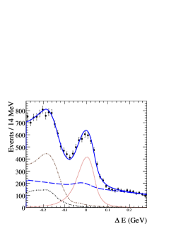
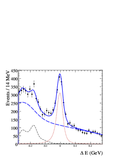
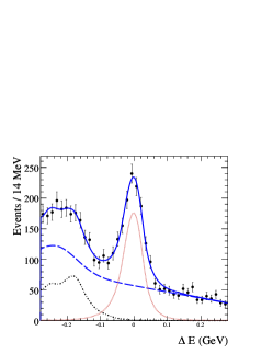
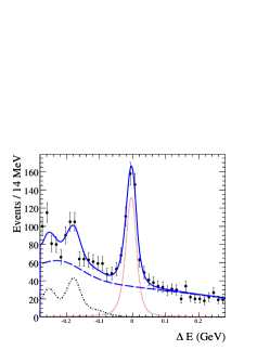
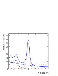
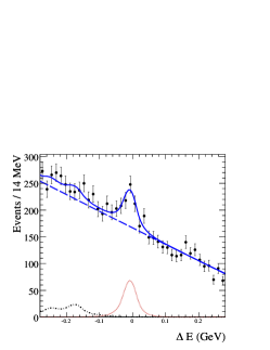
Figure 2: Fit of $\Delta E$ distributions in data for modes $\kern 1.79993pt\overline{\kern-1.79993ptB}{}^{0}\rightarrow D^{0}\pi^{0}$ (top left), $\kern 1.79993pt\overline{\kern-1.79993ptB}{}^{0}\rightarrow D^{0}\omega$ (top middle), $\kern 1.79993pt\overline{\kern-1.79993ptB}{}^{0}\rightarrow D^{0}\eta(\gamma\gamma)$ (top right), $\kern 1.79993pt\overline{\kern-1.79993ptB}{}^{0}\rightarrow D^{0}\eta(\pi\pi\pi^{0})$ (bottom left), $\kern 1.79993pt\overline{\kern-1.79993ptB}{}^{0}\rightarrow D^{0}\eta^{\prime}(\pi\pi\eta)$ (bottom middle) and $\kern 1.79993pt\overline{\kern-1.79993ptB}{}^{0}\rightarrow D^{0}\eta^{\prime}(\rho^{0}\gamma)$ (bottom right). The dots with error bars are data, the solid curve is the fitted total pdf, the dotted curve is the signal pdf, the dotted-dashed curve is the crossfeed pdf, the double dotted-dashed curve is the $B^{-}\rightarrow D^{(*)0}\rho^{-}$ pdf and the long dashed curve is the combinatorial background pdf.

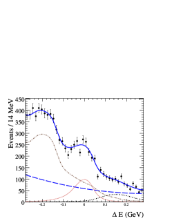
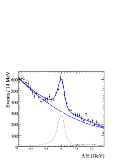
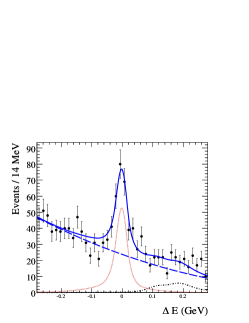
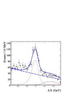
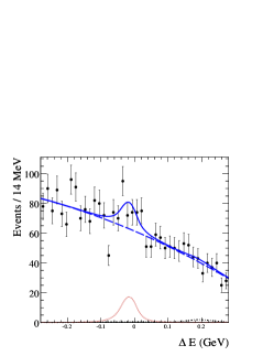
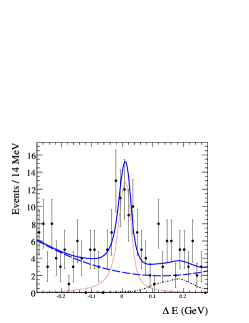
Figure 3: Fit of $\Delta E$ distributions in data for modes $\kern 1.79993pt\overline{\kern-1.79993ptB}{}^{0}\rightarrow D^{*0}\pi^{0}$ (top left), $\kern 1.79993pt\overline{\kern-1.79993ptB}{}^{0}\rightarrow D^{*0}\omega$ (top middle), $\kern 1.79993pt\overline{\kern-1.79993ptB}{}^{0}\rightarrow D^{*0}\eta(\pi\pi\pi^{0})$ (top right), $\kern 1.79993pt\overline{\kern-1.79993ptB}{}^{0}\rightarrow D^{*0}\eta(\gamma\gamma)$ (bottom left), $\kern 1.79993pt\overline{\kern-1.79993ptB}{}^{0}\rightarrow D^{*0}(D^{0}\pi^{0})\eta^{\prime}(\rho^{0}\gamma)$ (bottom middle) and $\kern 1.79993pt\overline{\kern-1.79993ptB}{}^{0}\rightarrow D^{*0}\eta^{\prime}(\pi\pi\eta)$ (bottom right). Detailed legend is provided in Figure 2.

The signal and background yields obtained from the fit to data are given in Table 2 with the corresponding statistical significances.

Table 2: We give the number of signal events ($S$), crossfeed ($N_{\textrm{cf}}$), $B^{-}\rightarrow D^{(*)0}\rho^{-}$ ($N_{\textrm{D}\rho}$) and combinatorial background ($N_{\textrm{combi}}$) from the $\Delta E$ fit of data, and the ${\cal BF}$ measured for each submode. The number of background events $N_{\textrm{cf}}$, $N_{\textrm{D}\rho}$, and $N_{\textrm{combi}}$ are computed from the fitted pdf in the window $|\mbox{$\Delta E$}|<100~{}\mathrm{\,Me\kern-0.80005ptV}$. The statistical significance is defined as $\sqrt{2ln(L_{S+B}/L_{B})}$, where $L_{S+B}$ is the likelihood of the fit in data for the hypothesis of a signal, while $L_{B}$ is the likelihood for the hypothesis of pure background only.

$\kern 1.43994pt\overline{\kern-1.43994ptB}{}^{0}$ mode	$S$	$N_{\textrm{cf}}$	$N_{\textrm{D}\rho}$	$N_{\textrm{combi}}$	${\cal BF}(\times 10^{-4})$	Statistical
(decay channel)					$\pm\textrm{stat.}\pm\textrm{syst.}$	significance
$D^{0}\pi^{0}$	3369 $\pm$ 102	135	440 $\pm$ 11	2585 $\pm$ 63	2.78 $\pm$ 0.08 $\pm$ 0.20	35.5
$D^{0}\eta(\gamma\gamma)$	1054 $\pm$ 49	44	-	823 $\pm$ 21	2.34 $\pm$ 0.11 $\pm$ 0.17	26.1
$D^{0}\eta(\pi\pi\pi^{0})$	454 $\pm$ 29	20	-	487 $\pm$ 15	2.51 $\pm$ 0.16 $\pm$ 0.17	20.3
$D^{0}\omega$	1400 $\pm$ 58	68	-	1648 $\pm$ 28	2.77 $\pm$ 0.13 $\pm$ 0.22	29.4
$D^{0}\eta^{\prime}(\pi\pi\eta(\gamma\gamma))$	134 $\pm$ 14	6	-	74 $\pm$ 6	1.29 $\pm$ 0.14 $\pm$ 0.09	14.7
$D^{0}\eta^{\prime}(\rho^{0}\gamma)$	290 $\pm$ 42	13	-	2382 $\pm$ 33	1.95 $\pm$ 0.29 $\pm$ 0.30	7.2
$D^{*0}\pi^{0}$	958 $\pm$ 73	121	1218 $\pm$ 41	844 $\pm$ 56	1.78 $\pm$ 0.13 $\pm$ 0.23	15.1
$D^{*0}\eta(\gamma\gamma)$	629 $\pm$ 39	33	-	525 $\pm$ 18	2.37 $\pm$ 0.15 $\pm$ 0.24	19.4
$D^{*0}\eta(\pi\pi\pi^{0})$	241 $\pm$ 25	11	-	341 $\pm$ 13	2.27 $\pm$ 0.23 $\pm$ 0.18	12.2
$D^{*0}\omega$	1692 $\pm$ 86	60	-	4507 $\pm$ 47	4.44 $\pm$ 0.23 $\pm$ 0.61	22.3
$D^{*0}\eta^{\prime}(\pi\pi\eta)$	61 $\pm$ 10	3	-	34 $\pm$ 4	1.12 $\pm$ 0.26 $\pm$ 0.27	8.0
$D^{*0}(D^{0}\pi^{0})\eta^{\prime}(\rho^{0}\gamma)$	86 $\pm$ 28	6	-	874 $\pm$ 20	1.64 $\pm$ 0.53 $\pm$ 0.20	3.3

4 SYSTEMATIC STUDIES

There are several sources of systematic uncertainty in this analysis. Table 3 summarizes the studied systematic uncertainties with their values in percentage of ${\cal BF}$ for the different modes $D^{(*)0}h^{0}$. The large uncertainties for $D^{*0}h^{0}$ mainly come from $D^{*0}(D^{0}\gamma)h^{0}$.

The categories “$\pi^{0}/\gamma$ detection” (“Tracking”) account for the systematics on the reconstruction of $\pi^{0}/\gamma$ and charged particle tracks, and are taken as the uncertainty on the efficiency correction computed in the study of $\tau$ decays (see Section 3.3.5).

Similarly, the systematic uncertainties on kaon identification and $K^{0}_{\scriptscriptstyle S}$ selections, are estimated from the uncertainties on MC efficiency corrections computed in the study of pure samples of kaons and $K^{0}_{\scriptscriptstyle S}$ mesons in data respectively (see Section 3.3.5).

The systematic errors on the submodes ${\cal BF}$ is a combination of the uncertainty on each $D^{0}$ and $h^{0}$ submode [24]. The correlation between the calibration mode $D^{0}\rightarrow K^{-}\pi^{+}$ and $D^{0}\rightarrow X$, $X\neq K^{-}\pi^{+}$ was accounted for.

The uncertainty related to the number of $B\kern 1.79993pt\overline{\kern-1.79993ptB}{}$ pairs and to the limited MC statistics is also included [9].

The systematics on resonance mass cut are computed as the relative difference of signal yield when the mass mean and resolution for the selection are taken from a fit in data.

The uncertainties for the $q\overline{q}$ rejection and the $D^{(*)0}$ selections are obtained from the study performed on the control sample $B^{-}\rightarrow D^{(*)0}\pi^{-}$ and are estimated as the uncertainty on the efficiency correction eff(data)$/$eff(MC), including the correlations between the samples before and after selections (see Section 3.3.5).

The uncertainties for the cuts on $\rho^{0}$ and $D^{0}\omega$ helicities are obtained by varying the selection cut values by $\pm 10~{}\%$ around the maximum of statistical significance.

The category “Signal shape” represents the uncertainty on the shape of the signal pdf for the $\Delta E$ fit. The expected shape difference between data and MC is estimated from a study of the control sample $B^{-}\rightarrow D^{(*)0}\rho^{-}$, hich gives: $|\Delta\textrm{mean}|\simeq 5.7~{}\mathrm{\,Me\kern-1.00006ptV}$ and $|\Delta\sigma|\simeq 2.3~{}\mathrm{\,Me\kern-1.00006ptV}$. The systematic on signal shape is obtained by varying the pdf parameters by $\pm 5.7~{}\mathrm{\,Me\kern-1.00006ptV}$ for the mean and $\pm 2.3~{}\mathrm{\,Me\kern-1.00006ptV}$ for the resolution.

The uncertainty on the continuum background shape is estimated from the difference of the pdf fitted on generic MC’s with the pdf fitted in the $m_{\rm ES}$ sideband $5.24<\mbox{$m_{\rm ES}$}<5.26~{}{\mathrm{\,Ge\kern-1.00006ptV\!/}c^{2}}$ in data. When a Gaussian is added to the combinatorial background shape, the related uncertainty is computed by varying its means and resolution by $\pm 1\sigma$.

The uncertainties related to the branching fractions of the crossfeed from $D^{(*)0}h^{0}$ and $D^{(*)0}\rho^{-}$ were computed by varying the ${\cal BF}$ separately by $\pm 1\sigma$ in the fit procedure. The value of $\sigma$ used is taken from the fit for $D^{(*)0}h^{0}$ and from PDG for $D^{(*)0}\rho^{-}$.

The uncertainty related to the crossfeed shape, modelled by a non-parametric pdf, is obtained by shifting and smearing the pdf mean and resolution by $\pm 5.7$ and 2.3 $\mathrm{\,Me\kern-1.00006ptV}$ respectively, with a convolution by a Gaussian.

The uncertainty in “$D^{*0}\omega$ helicity” accounts for the hypothesis on the $D^{*0}\omega$ polarization in the MC generation. As that polarization had never been measured, following HQET and factorization based arguments, the $D^{*0}\omega$ polarization was simulated using the helicity parameters measured in $B^{-}\rightarrow D^{*0}\rho^{-}$, thus a longitudinal fraction of $f_{L}=0.869$ [30], confirmed by a CLEO measurement [31]. That systematic is estimated by a comparison of the efficiency as obtained from an exclusive simulation of $\kern 1.79993pt\overline{\kern-1.79993ptB}{}^{0}\rightarrow D^{*0}\omega$ with a low $f_{L}$ value of $0.08$ and is taken as half of the relative difference of the signal yield.

The most significant systematic uncertainties come from the $\pi^{0}/\gamma$ reconstruction, the submodes ${\cal BF}$, the longitudinal fraction for $D^{*0}\omega$, from the signal and background parametrization on the $\Delta E$ fit and from the crossfeed by $D^{(*)0}\rho^{-}$.

Table 3: Systematic uncertainties ($\%$) for the modes $\kern 1.43994pt\overline{\kern-1.43994ptB}{}^{0}\rightarrow D^{(*)0}h^{0}$ where $D^{(*)0}$ submodes are summed.

	$D^{0}h^{0}$						$D^{*0}h^{0}$
Sources	$\pi^{0}$	$\eta(\gamma\gamma)$	$\eta(3\pi)$	$\omega$	$\eta^{\prime}(\pi\pi\eta)$	$\eta^{\prime}(\rho^{0}\gamma)$	$\pi^{0}$	$\eta(\gamma\gamma)$	$\eta(3\pi)$	$\omega$	$\eta^{\prime}(\pi\pi\eta)$	$\eta^{\prime}(\rho^{0}\gamma)$
$\pi^{0}/\gamma$ detection	4.0	4.0	4.0	4.0	4.0	2.4	5.9	5.9	6.1	6.1	5.8	4.5
PID	1.1	1.1	1.2	1.2	1.2	1.1	1.2	1.2	1.2	1.2	1.2	1.2
Tracking	0.9	0.9	1.6	1.6	1.6	1.6	0.9	0.9	1.6	1.6	1.5	1.5
$K^{0}_{\scriptscriptstyle S}$ selection	0.1	0.1	0.1	0.1	0.1	0.1	0.0	0.1	0.0	0.1	-	-
Submodes ${\cal BF}$	3.2	3.3	3.5	3.3	4.5	4.4	3.1	3.2	3.4	3.2	4.3	6.4
$B\kern 1.43994pt\overline{\kern-1.43994ptB}{}$ counting	1.1	1.1	1.1	1.1	1.1	1.1	1.1	1.1	1.1	1.1	1.1	1.1
$MC$ statistics	0.3	0.5	0.7	0.4	1.0	0.9	0.6	0.8	1.1	0.6	1.1	1.2
Resonances mass	0.5	0.7	0.4	0.1	0.7	0.7	0.5	0.7	0.4	0.1	0.7	0.7
$q\overline{q}$ rejection	0.2	0.2	0.2	0.2	0.2	0.2	0.2	0.2	0.2	0.2	0.2	0.2
$D^{(*)0}$ selection	0.3	0.3	0.3	0.3	0.3	0.3	0.4	0.4	0.4	0.4	0.4	0.4
$\rho^{0}$ helicity	-	-	-	-	-	2.1	-	-	-	-	-	2.1
$D^{(*)0}\omega$ helicity	-	-	-	1.9	-	-	-	-	-	10.8	-	-
Signal shape	2.6	2.8	1.5	1.7	1.3	2.7	1.9	2.8	1.8	3.3	1.0	3.1
Continuum shape	1.0	0.8	1.1	4.2	1.2	13.3	0.9	6.5	1.7	3.3	21.2	6.8
Crossfeed ${\cal BF}$	0.0	0.0	0.0	0.0	0.1	0.1	8.6	1.2	2.11	0.8	8.6	0.3
Crossfeed shape	0.7	0.7	0.3	0.6	0.5	0.4	6.1	0.2	0.3	0.2	0.6	0.2
Total	6.2	6.3	6.2	7.5	6.8	14.9	12.8	10.0	8.1	13.8	24.1	11.3

5 RESULTS

5.1 ${\cal BF}$ measurement

The branching fractions obtained from the $\Delta E$ fit on data are given in Table 2 for the sum of the $D^{(*)0}$ submodes. The consistency with $D^{0}$ submodes was checked. All the quoted results are the branching fraction ${\cal BF}_{\textrm{sum}}$ computed with the fit of the $D^{0}$ sum.

The statistical uncertainty $\sigma_{\textrm{stat}}$ on ${\cal BF}_{\textrm{sum}}$ is provided by the fit while the systematic uncertainty is computed as the average of the systematic weighted by the total corrected acceptance $\mathcal{A}_{i}$:

$$\sigma_{\textrm{syst}}=\frac{\sum_{i}\mathcal{A}_{i}\cdot\sigma_{\textrm{syst,}i}}{\sum_{i}\mathcal{A}_{i}},$$ (10)

where $({\cal BF}_{i}\pm\sigma_{\textrm{syst,}i}\pm\sigma_{\textrm{stat,}i})$ is the measured branching fraction with the submode $i=K^{-}\pi^{+}$, $K^{-}\pi^{+}\pi^{-}\pi^{+}$, $K^{-}\pi^{+}\pi^{0}$ or $K^{0}_{\scriptscriptstyle S}\pi^{+}\pi^{-}$. The total uncertainty is eventually computed as the quadrature sum of $\sigma_{\textrm{stat}}$ and $\sigma_{\textrm{syst}}$. We checked the compatibility of ${\cal BF}_{\textrm{sum}}$ with the measurements in the submodes ${\cal BF}_{i}$ for significant signal. The ${\cal BF}$’s measured with $D^{*0}$ submodes are compatible with ${\cal BF}_{\textrm{sum}}$, except for $\kern 1.79993pt\overline{\kern-1.79993ptB}{}^{0}\rightarrow D^{*0}\pi^{0}$ where the incompatibility between $D^{*0}\rightarrow D^{0}\gamma$ and $D^{*0}\rightarrow D^{0}\pi^{0}$ is due to the large background contribution from $D^{(*)0}\rho^{-}$. Likewise the measurements in the different $\eta$ or $\eta^{\prime}$ submodes are compatible. The measurements in the $\eta^{(^{\prime})}$ submodes are combined through a ${\cal BF}$ average weighted by the total uncertainty on ${\cal BF}$:

$${\cal BF}_{\textrm{avg}}=\frac{\sum_{i}{\cal BF}_{i}/\sigma_{i}^{2}}{\sum_{i}1/\sigma_{i}^{2}},$$ (11)

where $({\cal BF}_{i}\pm\sigma_{i})$ is the measured branching fraction with the submode $i$, and $\sigma_{i}$ the total uncertainty on ${\cal BF}_{i}$. The statistical uncertainty on the ${\cal BF}$ combination is :

$$\sigma^{2}_{\textrm{stat,avg}}=\sum_{i}\frac{1}{1/\sigma_{\textrm{stat,}i}^{2}},$$ (12)

and the systematic is obtained from the Equation (10).

The ${\cal BF}$’s measured in this analysis are compatible with the previous measurements by BABAR [9], CLEO [7] and Belle [10, 11]. For the modes $\kern 1.79993pt\overline{\kern-1.79993ptB}{}^{0}\rightarrow D^{(*)0}\eta$, $D^{*0}\omega$ and $D^{*0}(D^{0}\pi^{0})\pi^{0}$,

our measured ${\cal BF}$s are significantly higher than the ones measured by Belle [11]. We also measured the ${\cal BF}$ in the dataset studied previously by BABAR [9] and found compatible ${\cal BF}$ values with systematic uncertainties lowered by about 25 to 50 $\%$. The improvement mainly comes from the selections on $D^{(*)0}$ and on the $q\overline{q}$ background rejection.

5.2 Isospin analysis

The isospin $I$ symmetry relates the amplitudes of the decays $B^{-}\rightarrow D^{(*)0}\pi^{-}$, $\kern 1.79993pt\overline{\kern-1.79993ptB}{}^{0}\rightarrow D^{(*)+}\pi^{-}$ and $\kern 1.79993pt\overline{\kern-1.79993ptB}{}^{0}\rightarrow D^{(*)0}\pi^{0}$, which can be written as linear combinations of the isospin eigenstates $\mathcal{A}_{I}$, $I=1/2$, $3/2$ [4, 33]:

$$\mathcal{A}(D^{(*)0}\pi^{-})= \sqrt{3}\mathcal{A}_{3/2,D^{(*)}},$$ (13)

$$\mathcal{A}(D^{(*)+}\pi^{-})= 1/\sqrt{3}\mathcal{A}_{3/2,D^{(*)}}+\sqrt{2/3}\mathcal{A}_{1/2,D^{(*)}},$$

$$\mathcal{A}(D^{(*)0}\pi^{0})= \sqrt{2/3}\mathcal{A}_{3/2,D^{(*)}}-\sqrt{1/3}\mathcal{A}_{1/2,D^{(*)}},$$

and so:

$$\mathcal{A}(D^{(*)0}\pi^{-})=\mathcal{A}(D^{(*)+}\pi^{-})+\sqrt{2}\mathcal{A}(D^{(*)0}\pi^{0}).$$ (14)

The relative strong phase between the eigenstates $\mathcal{A}_{1/2}$ and $\mathcal{A}_{3/2}$ is noted as $\delta$ for the $D\pi$ system and $\delta^{*}$ for $D^{*}\pi$ system. Final State Interactions between the states $D^{(*)0}\pi^{0}$ and $D^{(*)+}\pi^{-}$ may lead to a value of $\delta^{(*)}$ different from zero and, through constructive interference, to a higher value of ${\cal BF}$ for $D^{(*)0}\pi^{0}$. One can also define the amplitude ratio $R^{(*)}$:

$$R^{(*)}=\frac{|\mathcal{A}^{(*)}_{1/2}|}{\sqrt{2}|\mathcal{A}^{(*)}_{3/2}|}.$$ (15)

In the HQET limit [36, 38], the factorization model predicts $\delta^{(*)}=0$ and $R^{(*)}=1$, while SCET [16, 17, 18] predicts $\delta$ to have the same value in the $D\pi$ and $D^{*}\pi$ systems. The strong phase $\delta^{(*)}$ can be computed with an isospin analysis of the $D^{(*)}\pi$ system. The input parameters are the world average values provided by the PDG 2007 partial update [24] of ${\cal BF}(B^{-}\rightarrow D^{(*)0}\pi^{-})$, ${\cal BF}(\kern 1.79993pt\overline{\kern-1.79993ptB}{}^{0}\rightarrow D^{(*)+}\pi^{-})$ and of the $B$ lifetime ratio $\tau(B^{+})/\tau(B^{0})$, the value of ${\cal BF}(\kern 1.79993pt\overline{\kern-1.79993ptB}{}^{0}\rightarrow D^{(*)0}\pi^{0})$ is the one measured in this analysis. We calculate the value of $\delta^{(*)}$ and $R^{(*)}$ using a frequentist approach [37] $\delta=(30.2^{+3.2}_{-4.5})^{\circ}$ and $R=0.70^{+0.05}_{-0.05}$ for $D\pi$ final states, and $\delta^{*}=(13.6^{+9.9}_{-13.6})^{\circ}$, $R^{*}=0.64^{+0.06}_{-0.05}$ for $D^{*}\pi$ final states.

In both $D^{*}\pi$ and $D\pi$ cases, the amplitude ratio is significantly different from the factorization prediction $R^{(*)}=1$. The strong phase is significantly different from zero in the system $D\pi$, which points out that non-factorizable FSI are not negligible. In the system $D^{*}\pi$ that phase $\delta^{*}$ is smaller and compatible with zero due to the lower value of the ${\cal BF}$ for $D^{*0}\pi^{0}$.

5.3 Comparison to theoretical predictions on ${\cal BF}$’s

Table 4 compares the ${\cal BF}$ measured with this analysis to the predictions by factorization [13, 2, 34, 35] and pQCD [14, 15]. We confirm the conclusion by the previous BABAR analysis, the values measured being higher by a factor of about 4 than the values predicted by factorization. The pQCD predictions are closer to experimental values but globally higher except for $D^{0}\pi^{0}$.

Table 4: Comparison of the measured branching fraction ${\cal BF}$ in units of $10^{-4}$, with the predictions by factorization and pQCD [14, 15]. The first quoted uncertainty is statistical and the second is systematic.

$\kern 1.43994pt\overline{\kern-1.43994ptB}{}^{0}$ mode	This measurement $(\times 10^{-4})$	factorization $(\times 10^{-4})$	pQCD $(\times 10^{-4})$
$D^{0}\pi^{0}$	2.78 $\pm$ 0.08 $\pm$ 0.20	0.58 [13] 0.70 [2]	2.3-2.6
$D^{*0}\pi^{0}$	1.78 $\pm$ 0.13$\pm$ 0.23	0.65 [13] 1.00 [2]	2.7-2.9
$D^{0}\eta$	2.41 $\pm$ 0.09 $\pm$ 0.17	0.34 [13] 0.50 [2]	2.4-3.2
$D^{*0}\eta$	2.32 $\pm$ 0.13 $\pm$ 0.22	0.60 [2]	2.8-3.8
$D^{0}\omega$	2.77 $\pm$ 0.13 $\pm$ 0.22	0.66 [13] 0.70 [2]	5.0-5.6
$D^{*0}\omega$	4.44 $\pm$ 0.23 $\pm$ 0.61	1.70 [2]	4.9-5.8
$D^{0}\eta^{\prime}$	1.38 $\pm$ 0.12 $\pm$ 0.22	0.30-0.32 [35]; 1.70-3.30 [34]	1.7-2.6
$D^{*0}\eta^{\prime}$	1.29 $\pm$ 0.23 $\pm$ 0.23	0.41-0.47 [34]	2.0-3.2

Factorization predicts the ratio ${\cal BF}(\kern 1.79993pt\overline{\kern-1.79993ptB}{}^{0}\rightarrow D^{(*)0}\eta^{\prime})/{\cal BF}(\kern 1.79993pt\overline{\kern-1.79993ptB}{}^{0}\rightarrow D^{(*)0}\eta)$ to have a value between 0.64 and 0.68 [34] linked to the $\eta-\eta^{\prime}$ mixing. Table 5 compares that prediction with the experimental measurements. The measured ratios are smaller than the prediction and are compatible at 1 $\sigma$.

The effective theory SCET [16, 17, 18] does not predict the absolute value of the ${\cal BF}$ but that the ratios ${\cal BF}(\kern 1.79993pt\overline{\kern-1.79993ptB}{}^{0}\rightarrow D^{*0}h^{0})/{\cal BF}(\kern 1.79993pt\overline{\kern-1.79993ptB}{}^{0}\rightarrow D^{0}h^{0})\sim 1$ for $h^{0}=\pi^{0},\eta$ and $\eta^{\prime}$. For $h^{0}=\omega$ that prediction holds only for the longitudinal component of $\kern 1.79993pt\overline{\kern-1.79993ptB}{}^{0}\rightarrow D^{*0}\omega$ as long-distance QCD interactions may increase the transverse amplitude. A measurement of $f_{L}$ is therefor needed.

The SCET gives also a prediction about the ratio ${\cal BF}(\kern 1.79993pt\overline{\kern-1.79993ptB}{}^{0}\rightarrow D^{(*)0}\eta^{\prime})/{\cal BF}(\kern 1.79993pt\overline{\kern-1.79993ptB}{}^{0}\rightarrow D^{(*)0}\eta)\simeq 0.67$, which is similar to the prediction by factorization.

The ${\cal BF}$ ratios are given in Table 5, the common systematics between $D^{0}h^{0}$ and $D^{*0}h^{0}$ are cancelled. The ratios ${\cal BF}(\kern 1.79993pt\overline{\kern-1.79993ptB}{}^{0}\rightarrow D^{*0}h^{0})/{\cal BF}(\kern 1.79993pt\overline{\kern-1.79993ptB}{}^{0}\rightarrow D^{0}h^{0})$ for $h^{0}=\pi^{0},\eta,\eta^{\prime}$ are compatible with 1.

Table 5: Ratios of branching fractions ${\cal BF}(\kern 1.43994pt\overline{\kern-1.43994ptB}{}^{0}\rightarrow D^{*0}h^{0})/{\cal BF}(\kern 1.43994pt\overline{\kern-1.43994ptB}{}^{0}\rightarrow D^{0}h^{0})$. The first uncertainty is statistical, the second is systematic.

${\cal BF}$ ratio	This measurement
$\frac{{\cal BF}(D^{*0}\pi^{0})}{{\cal BF}(D^{0}\pi^{0})}$	0.64 $\pm$ 0.05 $\pm$ 0.08
$\frac{{\cal BF}(D^{*0}\eta(\gamma\gamma))}{{\cal BF}(D^{0}\eta(\gamma\gamma))}$	1.01 $\pm$ 0.08 $\pm$ 0.08
$\frac{{\cal BF}(D^{*0}\eta(\pi\pi\pi^{0}))}{{\cal BF}(D^{0}\eta(\pi\pi\pi^{0}))}$	0.91 $\pm$ 0.11 $\pm$ 0.04
$\frac{{\cal BF}(D^{*0}\eta)}{{\cal BF}(D^{0}\eta)}$	0.96 $\pm$ 0.06 $\pm$ 0.07
$\frac{{\cal BF}(D^{*0}\omega)}{{\cal BF}(D^{0}\omega)}$	1.61 $\pm$ 0.11 $\pm$ 0.20
$\frac{{\cal BF}(D^{*0}\eta^{\prime}(\pi\pi\eta))}{{\cal BF}(D^{0}\eta^{\prime}(\pi\pi\eta))}$	0.87 $\pm$ 0.22 $\pm$ 0.04
$\frac{{\cal BF}(D^{*0}\eta^{\prime}(\rho^{0}\gamma))}{{\cal BF}(D^{0}\eta^{\prime}(\rho^{0}\gamma)))}$	0.84 $\pm$ 0.30 $\pm$ 0.15
$\frac{{\cal BF}(D^{*0}\eta^{\prime})}{{\cal BF}(D^{0}\eta^{\prime}))}$	0.93 $\pm$ 0.19 $\pm$ 0.11
$\frac{{\cal BF}(D^{0}\eta^{\prime})}{{\cal BF}(D^{0}\eta)}$	0.57 $\pm$ 0.06 $\pm$ 0.06
$\frac{{\cal BF}(D^{*0}\eta^{\prime})}{{\cal BF}(D^{*0}\eta)}$	0.55 $\pm$ 0.11 $\pm$ 0.04

6 CONCLUSIONS

We measured the branching fractions of the color-suppressed decays $\kern 1.79993pt\overline{\kern-1.79993ptB}{}^{0}\rightarrow D^{(*)0}h^{0}$, where $h^{0}=\pi^{0}$, $\eta$, $\omega$, and $\eta^{\prime}$ with 454$\times 10^{6}B\kern 1.79993pt\overline{\kern-1.79993ptB}{}$ pairs. Our measurements are in agreement with the previous results [7, 9, 10] with a significant decrease of both statistical and systematic uncertainties. We confirm the significant difference from theoretical predictions by factorization quoted in the previous analysis [9] and provide strong constraints on the models of color-suppressed decays.

7 ACKNOWLEDGMENTS

We are grateful for the excellent luminosity and machine conditions provided by our PEP-II colleagues, and for the substantial dedicated effort from the computing organizations that support BABAR. The collaborating institutions wish to thank SLAC for its support and kind hospitality. This work is supported by DOE and NSF (USA), NSERC (Canada), CEA and CNRS-IN2P3 (France), BMBF and DFG (Germany), INFN (Italy), FOM (The Netherlands), NFR (Norway), MES (Russia), MEC (Spain), and STFC (United Kingdom). Individuals have received support from the Marie Curie EIF (European Union) and the A. P. Sloan Foundation.

References

- [1] D. Du, Phys. Lett. B 406, 110 (1997).
- [2] M. Neubert and B. Stech, in Heavy Flavours II, eds. A.J. Buras and M. Lindner (World Scientific, Singapore, 1998), p. 294.
- [3] M. Bauer, B. Stech and M. Wirbel, Z. Phys. C 34, 103 (1987).
- [4] M. Neubert and A.A. Petrov, Phys. Lett. B 519, 50 (2001).
- [5] A. Deandrea, N. Di Bartolomeo, R. Gatto, and G. Nardulli, Phys. Lett. B 318, 549 (1993); A. Deandrea et al., 320, 170 (1994).
- [6] K. Honscheid, K. R. Schubert, and R. Waldi, Z. Phys. C 63, 117 (1994).
- [7] CLEO Collaboration, T. E. Coan et al., Phys. Rev. Lett. 88, 062001 (2002).
- [8] Belle Collaboration, K. Abe et al., Phys. Rev. Lett. 88, 052002 (2002).
- [9] BABAR Collaboration, B. Aubert et al., Phys. Rev. D 69, 032004 (2004).
- [10] Belle Collaboration, J. Sch mann et al., Phys. Rev. D 72, 011103 (2005).
- [11] Belle Collaboration, K. Abe et al., Phys. Rev. D 74, 092002 2006).
- [12] Belle Collaboration, K. Abe et al., (2007), Phys. Rev. D 76, 012006 (2007).
- [13] C-K. Chua, W-S. Hou, and K-C. Yang, Phys. Rev. D 65, 096007 (2002).
- [14] Y.Y Keum, T. Kurimoto, H. Li, C.D Lü and A.I. Sanda, Phys. Rev. D 69, 094018 (2004).
- [15] C.D Lü, Phys. Rev. D 68, 097502 (2003).
- [16] C. W. Bauer, D. Pirjol and I. W. Stewart, Phys. Rev. D 65, 054022 (2002).
- [17] A.E. Blechman, S. Mantry and I.W. Stewart, Phys. Lett. B 608, 77 (2005).
- [18] S. Mantry, D. Pirjol and I. W. Stewart, Phys. Rev. D 68 114009 (2003), MIT-CTP-3370.
- [19] BABAR Collaboration, B. Aubert et al., Nucl. Instrum. Methods Phys. Res., Sect. A 479, 1 (2002).
- [20] D. Lange, Nucl. Instrum. Methods Phys. Res., Sect. A 462, 152 (2001).
- [21] T. Sjostrand, S. Mrenna and P. Skands, Comput. Phys. Commun. 178, 852 (2008).
- [22] T. Sjöstrand, Comput. Phys. Commun. 82, 74 (1994).
- [23] Collaboration, V. N. Ivanchenko et al., Nucl. Instrum. Methods Phys. Res., Sect. A 494, 514 (2002). Collaboration, S. Agostinelli et al., ibid. 506, 250 (2003).
- [24] Particle Data Group, W.-M. Yao et al., J. Phys. G 33, 1 (2006), and partial 2007 update for the 2008 edition.
- [25] Collaboration E691, J.C. ANJOS et al., Phys. Rev. D 48, 56 (1993).
- [26] A. Höcker et al., TMVA Group, [arXiv:physics/0703039v4] (2007).
- [27] BABARnote 870.
- [28] BABARnote 87 and 867.
-
[29]
The modified Novossibirsk function divides the
fitting region in a peaking region, a low and a high tail
regions. For a variable , the modified Novosibirsk function
is:
in the peak region : ,
in the low tail region: ,(16)
in the high tail region: ,(17)
The parameters are:(18) -
•
is the value at the maximum of the function,
-
•
is the peak position,
-
•
is the width of the peak defined as the width at half-height divided by 2.35.
-
•
is an asymmetry parameter.
-
•
- [30] CLEO Collaboration, G. Bonvicini et al., CLEO CONF 98-23, ICHEP98 852, Proceedings of XXVIV ICHEP, Vancouver, 1998.
- [31] CLEO Collaboration, S.E. Csorna et al., Phys. Rev. D 67, 112002 (2003).
- [32] S.M. Berman, M. Jacob, Phys. Rev. Lett. 139, 1023 (1965).
- [33] J.L. Rosner, Phys. Rev. D 60, 074028 (1999).
- [34] A. Deandrea and A.D. Polosa, Eur. Phys. Jour. 22, 677 (2002).
- [35] J.O. Eeg, A. Hiorth and A.D. Polosa, Phys. Rev. D 65, 054030 (2002).
- [36] M. Beneke, G. Buchalla, M. Neubert and C. T. Sachradja, Nucl. Phys. B 591, 313 (2000).
- [37] CKMfitter Group (J. Charles et al.), Eur. Phys. Jour. C 41, 1-131 (2005).
- [38] H-Y. Cheng and K-C Yang, Phys. Rev. D 59, 092004 (1999).