$n$-dimensional ratio-dependent predator-prey systems with memory

Abstract

This paper deals with ratio-dependent predator-prey systems with delay. We will investigate under what conditions delay cannot cause instability in higher dimension. We give an example when delay causes instability.

Key words and phrases: predator-prey system, functional response, sign stability, ratio dependence, delay

1 Introduction

Let us consider the following ratio-dependent ecological system, in which $n$ different predator species (the $i$-th predator quantities at time $t$ are denoted by $y_{i}(t)$, $i=1,2,\dots,n$ respectively) are competing for a single prey species (the quantity of prey at time $t$ is denoted by $x(t)$):

$$\left.\begin{array}[]{lll}\dot{x}&=&rxg(x,K)-\displaystyle\sum_{i=1}^{n}y_{i}p_{i}\left(\frac{y_{i}}{x}\right)\\ \dot{y}_{i}&=&y_{i}p_{i}\displaystyle\left(\frac{y_{i}}{x}\right)-d_{i}y_{i},\quad i=1,2,\dots,n\end{array}\right\}.$$ (1)

where dot means differentiation with respect to time $t$. We assume that the per capita growth rate of prey in absence of predators is $rg(x,K)$ where $r$ is a positive constant (in fact the maximal growth rate of prey), $K>0$ is the carrying capacity of environment with respect to the prey, the function $g$ satisfies some natural conditions, see the details in [6]. For example one of these conditions is the following:

$$(K-x)g(x,K)>0,\;\;x\geq 0,\;\;x\neq K.$$ (2)

Such a function $g$ is the so called logistic growth rate of prey

$$g(x,K)=1-\frac{x}{K}.$$ (3)

We assume further that the death rate $d_{i}>0$ of predator $i$ is constant and the per capita birth rate of the same predator is $p_{i}\left(\displaystyle\frac{y_{i}}{x}\right)$, where the function $p_{i}$ also satisfies some natural conditions, see also in [6].

In that paper we have already investigated the system with the Michaelis–Menten or Holling type functional response in case of ratio-dependence:

$$p_{i}\left(\frac{y_{i}}{x},a_{i}\right)=m_{i}\frac{x}{a_{i}y_{i}+x}.$$ (4)

and with the ratio-dependent Ivlev functional response:

$$p_{i}\left(\frac{y_{i}}{x},a_{i}\right)=m_{i}\left(1-e^{-\frac{x}{a_{i}y_{i}}}\right),$$ (5)

where parameter $a_{i}$ is the so called ”half-saturation constant”, namely in the case where $p_{i}$ is a bounded function for fixed $a_{i}>0$, $m_{i}=\sup\limits_{x,y_{i}>0}p_{i}(x,y_{i},a_{i})$ is the ”maximal birth rate” of the $i$-th predator. That means, if the functional response is a Holling-type without ratio-dependence then $a_{i}$ means the quantity of prey at which the birth rate of predator $i$ is half of its supremum. In case of a ratio-dependent Holling model $a_{i}$ means a proportion of prey to predator at which the birth rate is half of its supremum. In case of an Ivlev model the meaning of $a_{i}$ is similar to the earlier, see the details in [6]. (To save space we did not write out the dependence on $a_{i}$ in (1).) For the survival of predator $i$ it is, clearly, necessary that the maximal birth rate be larger, than the death rate:

$$m_{i}>d_{i}.$$ (6)

This will be assumed in the sequel. Finally, we assume that the presence of predators decreases the growth rate of prey by the amount equal to the birth rate of the respective predator.

2 Model with delay

We get a more realistic model if we take into account that the predators’ growth rate at present depend on past quantities of prey and therefore a continuous weight (or density) function $f$ is introduced whose role is to weight moments of the past. Function $f$ satisfies the requirements:

$$f(s)\geq 0,\;\;s\in(0,\infty);\;\;\int_{0}^{\infty}f(s)ds=1,$$ (7)

and $x(t)$ is replaced in the growth rate of predator $i$ by its weighted average over the past:

$$q(t):=\int_{-\infty}^{t}x(\tau)f(t-\tau)d\tau.$$ (8)

This means that the time average of prey quantity over the past has the same fading influence on the present growth rates of different predators. The simplest choice is $f(s)=\alpha e^{-\alpha s}$, with $\alpha>0$. This function satisfies the condition (7) and now

$$q(t)=\int_{-\infty}^{t}x(\tau)\alpha e^{-\alpha(t-\tau)}d\tau.$$ (9)

We call this choice of $f$ exponentially fading memory, see in [2], [7]; later in [4]. (Since $f$ is the probability density of an exponentially distributed random variable, the probabilistic interpretation is obvious.) The smaller $\alpha>0$ is the longer is the time interval in the past in which the values of $x$ are taken into account, i.e. $\frac{1}{\alpha}$ is the ”measure of the influence of the past”. It is easy to see that with this special delay, system (1) is equivalent to the following system of ordinary differential equations:

$$\left.\begin{array}[]{lll}\dot{x}&=&rxg(x,K)-\displaystyle\sum_{i=1}^{n}y_{i}p_{i}\left(\frac{y_{i}}{x}\right)\\ \dot{y}_{i}&=&y_{i}p_{i}\displaystyle\left(\frac{y_{i}}{q}\right)-d_{i}y_{i},\quad i=1,2,\dots,n\\ \dot{q}&=&\alpha(x-q)\end{array}\right\},$$ (10)

where function $p_{i}(\frac{y_{i}}{q})$ can be (4),(5) or any kind of general ratio-dependent functional response if we replace $x(t)$ by the time average $q(t)$ of prey quantity over the past. Similar systems have been studied by many authors in the two-dimensional case, specially in [1], and also with diffusion in [8]. In [1] the functional response was of the simplest Holling-type one without ratio-dependence and in [8] the functional response was of the Michaelis–Menten-type with ratio-dependence and also with diffusion. Our aim in this paper is to study the effect of exponentially fading memory in case of a general ratio-dependent functional response with more than one different predators.
The qualitative behaviour of (1) was studied in [6], where it has been supposed that there exists an equilibrium point $E^{*}(x^{*},y_{1}^{*},\dots,y_{n}^{*})$ in the positive orthant, where $x^{*}$, and $y_{i}^{*}$ are the solutions of the following equations:

$$rxg(x,K)=\sum_{i=1}^{n}d_{i}y_{i},\quad p_{i}\displaystyle\left(\frac{y_{i}}{x}\right)=d_{i},\quad i=1,\ldots,n.$$ (11)

Note that $x^{*}>0$ if and only if $K>x^{*}$ because of (2).
The coefficient matrix of the system (1) linearized at $E^{*}$ is:

$$A=\left[\begin{array}[]{cccccc}a_{11}&-d_{1}-y_{1}^{*}p^{\prime*}_{1}\frac{1}{x^{*}}&-d_{1}-y_{2}^{*}p^{\prime*}_{2}\frac{1}{x^{*}}&\dots&\dots&-d_{n}-y_{n}^{*}p^{\prime*}_{n}\frac{1}{x^{*}}\\ y_{1}^{*}p^{\prime*}_{1}(-\frac{y_{1}^{*}}{{x^{*}}^{2}})&y_{1}^{*}p^{\prime*}_{1}\frac{1}{x^{*}}&0&\dots&\dots&0\\ y_{2}^{*}p^{\prime*}_{2}(-\frac{y_{2}^{*}}{{x^{*}}^{2}})&0&y_{2}^{*}p^{\prime*}_{2}\frac{1}{x^{*}}&\dots&\dots&0\\ \vdots&\vdots&\vdots&\vdots&\vdots&\vdots\\ y_{{n-1}}^{*}p^{\prime*}_{{n-1}}(-\frac{y_{{n-1}}^{*}}{{x^{*}}^{2}})&0&0&\dots&y_{n-1}^{*}p^{\prime*}_{n-1}\frac{1}{x^{*}}&0\\ y_{n}^{*}p^{\prime*}_{n}(-\frac{y_{n}^{*}}{{x^{*}}^{2}})&0&0&\dots&0&y_{n}^{*}p^{\prime*}_{n}\frac{1}{x^{*}}\end{array}\right]$$ (12)

where

$$a_{11} = rg(x^{*},K)+rx^{*}g^{\prime}_{x}(x^{*},K)-\sum_{i=1}^{n}y_{i}^{*}p^{\prime*}_{i}(-\frac{y_{i}^{*}}{{x^{*}}^{2}}),$$ (13)

$$p^{\prime*}_{i} = p^{\prime}_{i}\displaystyle\left(\frac{{y_{i}}^{*}}{x^{*}}\right);\;\;p^{\prime}_{i}\displaystyle\left(\frac{y_{i}}{x}\right)=\frac{dp_{i}\left(\frac{y_{i}}{x}\right)}{d\left(\frac{y_{i}}{x}\right)}.$$ (14)

An $n\times n$ matrix $A=[a_{ij}]$ is said to be stable if each of its eigenvalues has a negative real part. The following definition can be found in [5]:

Definition 2.1.

An $n\times n$ matrix $A=[a_{ij}]$ is called sign-stable if each matrix $\tilde{A}$ of the same sign-pattern as $A$ ($\operatorname*{sign}\tilde{a}_{ij}=\operatorname*{sign}a_{ij}$ for all $i,j$) is stable.

It was proven in [6] the following:

Theorem 2.1.

If

$$a_{11}\leq 0,$$ (15)

$${p^{\prime}_{i}}^{*}=p^{\prime}_{i}\left(\frac{{y_{i}}^{*}}{x^{*}}\right)<0,\quad i=1,\ldots,n,$$ (16)

and

$$-d_{i}-{y_{i}}^{*}{p^{\prime}_{i}}^{*}\frac{1}{x^{*}}=-d_{i}-{y_{i}}^{*}p^{\prime}_{i}\left(\frac{{y_{i}}^{*}}{x^{*}}\right)\frac{1}{x^{*}}<0,\quad i=1,\ldots,n$$ (17)

then matrix (12) is sign-stable, thus, $E^{*}$ is an asymptotically stable equilibrium point of system (1).

Now, let us suppose that there exists a positive equilibrium point $E^{*}(x^{*},y_{1}^{*},\dots,y_{n}^{*})$ of system (1), then with the definition $q^{*}:=x^{*}$ and $E^{*}_{d}(x^{*},y_{1}^{*},\dots,y_{n}^{*},q^{*})$ we get an equilibrium point of (10) in the positive orthant. And again $x^{*}>0$ if and only if $K>x^{*}$.
The coefficient matrix of system (10) linearized at $E^{*}_{d}$ is:

$$A_{d}=\left[\begin{array}[]{cccccc}a_{11}&-d_{1}-y_{1}^{*}p^{\prime*}_{1}\frac{1}{x^{*}}&-d_{2}-y_{2}^{*}p^{\prime*}_{2}\frac{1}{x^{*}}\dots&\dots&-d_{n}-y_{n}^{*}p^{\prime*}_{n}\frac{1}{x^{*}}&0\\ 0&y_{1}^{*}p^{\prime*}_{1}\frac{1}{x^{*}}&0&\dots&0&y_{1}^{*}p^{\prime*}_{1}(-\frac{y_{1}^{*}}{{x^{*}}^{2}})\\ 0&0&y_{2}^{*}p^{\prime*}_{2}\frac{1}{x^{*}}&\dots&0&y_{2}^{*}p^{\prime*}_{2}(-\frac{y_{2}^{*}}{{x^{*}}^{2}})\\ \vdots&\vdots&\vdots&\vdots&\vdots&\vdots\\ 0&\dots&\dots&0&y_{n}^{*}p^{\prime*}_{n}\frac{1}{x^{*}}&y_{n}^{*}p^{\prime*}_{n}(-\frac{y_{n}^{*}}{{x^{*}}^{2}})\\ \alpha&0&\dots&\dots&0&-\alpha\end{array}\right]$$ (18)

where $a_{11}$ is given by (13) and again ${p^{\prime}_{i}}^{*}=p^{\prime}_{i}\displaystyle\left(\frac{{y_{i}}^{*}}{x^{*}}\right);\;\;p^{\prime}_{i}\displaystyle\left(\frac{y_{i}}{x}\right)=\frac{dp_{i}\left(\frac{y_{i}}{x}\right)}{d\left(\frac{y_{i}}{x}\right)}$.
We note that (18) can not be sign-stable because its graph have cycles. (See in [5].)

Let us restrict the number of predators to two.

2.1 One prey two predators with delay

Let us consider system (10) in case of $n=2$. We suppose that (15),(16), (17) hold for $i=1,2$. In this special case the entries of matrix $A_{d}$ are $a_{11}\leq 0$, $a_{22},a_{33}<0$, $a_{12},a_{13}<0$, $a_{24},a_{34}>0$, $a_{41}=\alpha>0$, $a_{44}=-\alpha<0$. This means that $A_{d}$ has the following sign pattern:

$$A_{d}=\left[\begin{array}[]{cccc}-/0&-&-&0\\ 0&-&0&+\\ 0&0&-&+\\ \alpha&0&0&-\alpha\end{array}\right].$$ (19)

The characteristic polynomial of a matrix with the same sign pattern as (19) is:

$$D(\lambda)=\lambda^{4}+a_{3}\lambda^{3}+a_{2}\lambda^{2}+a_{1}\lambda+a_{0}$$ (20)

with

$$a_{3}=-a_{11}-a_{22}-a_{33}+\alpha,$$

$$a_{2}=a_{11}a_{22}+a_{11}a_{33}+a_{22}a_{33}-\alpha(a_{11}+a_{22}+a_{33}),$$

$$a_{1}=-a_{11}a_{22}a_{33}+\alpha(a_{11}a_{22}+a_{11}a_{33}+a_{22}a_{33})-\alpha(a_{12}a_{24}+a_{13}a_{34}),$$

$$a_{0}=\det A_{d}=\alpha(-a_{11}a_{22}a_{33}+a_{22}a_{13}a_{34}+a_{33}a_{12}a_{24}).$$

It is known that the necessary condition of stability of the polynomial $D(\lambda)$ is $a_{i}>0,\;\;i=0,1,2,3$.

Lemma 2.1.

If $A_{d}$ has the same sign pattern as (19) then the above necessary conditions of stability are satisfied for all $\alpha>0$.

Proof.

It is an elementary calculation to prove $a_{i}>0,\;\;i=0,1,2,3$, for all $\alpha>0$. ∎

Sufficient condition of stability of matrix $A_{d}$ in this case is:

$$a_{3}(a_{1}a_{2}-a_{0}a_{3})-a_{1}^{2}>0$$ (21)

See for example Theorem 1.4.8 in [3]. It leads to a very complicated formula. In order to check this we used Wolfram Mathematica 6.0. http://www.wolfram.com. We got:
$H(\alpha)=a_{3}(a_{1}a_{2}-a_{0}a_{3})-a_{1}^{2}=$
$(-a_{22}a_{11}^{2}-a_{33}a_{11}^{2}-a_{22}^{2}a_{11}-a_{33}^{2}a_{11}+a_{12}a_{24}a_{11}-2a_{22}a_{33}a_{11}+a_{13}a_{34}a_{11}$ $-a_{22}a_{33}^{2}+a_{12}a_{22}a_{24}-a_{22}^{2}a_{33}+a_{13}a_{33}a_{34})\;\alpha^{3}$
$+(a_{22}a_{11}^{3}+a_{33}a_{11}^{3}+2a_{22}^{2}a_{11}^{2}+2a_{33}^{2}a_{11}^{2}-a_{12}a_{24}a_{11}^{2}+4a_{22}a_{33}a_{11}^{2}-a_{13}a_{34}a_{11}^{2}+a_{22}^{3}a_{11}+a_{33}^{3}a_{11}+4a_{22}a_{33}^{2}a_{11}-a_{12}a_{22}a_{24}a_{11}+4a_{22}^{2}a_{33}a_{11}+a_{12}a_{24}a_{33}a_{11}+a_{13}a_{22}a_{34}a_{11}-a_{13}a_{33}a_{34}a_{11}+a_{22}a_{33}^{3}-a_{12}^{2}a_{24}^{2}+2a_{22}^{2}a_{33}^{2}+a_{12}a_{24}a_{33}^{2}-a_{13}^{2}a_{34}^{2}-a_{12}a_{22}^{2}a_{24}+a_{22}^{3}a_{33}+a_{12}a_{22}a_{24}a_{33}+a_{13}a_{22}^{2}a_{34}-a_{13}a_{33}^{2}a_{34}-2a_{12}a_{13}a_{24}a_{34}+a_{13}a_{22}a_{33}a_{34})\;\alpha^{2}$
$+(-a_{22}^{2}a_{11}^{3}-a_{33}^{2}a_{11}^{3}-2a_{22}a_{33}a_{11}^{3}-a_{22}^{3}a_{11}^{2}-a_{33}^{3}a_{11}^{2}-4a_{22}a_{33}^{2}a_{11}^{2}+a_{12}a_{22}a_{24}a_{11}^{2}-4a_{22}^{2}a_{33}a_{11}^{2}+a_{13}a_{33}a_{34}a_{11}^{2}-2a_{22}a_{33}^{3}a_{11}-4a_{22}^{2}a_{33}^{2}a_{11}-a_{12}a_{24}a_{33}^{2}a_{11}+a_{12}a_{22}^{2}a_{24}a_{11}-2a_{22}^{3}a_{33}a_{11}-a_{12}a_{22}a_{24}a_{33}a_{11}-a_{13}a_{22}^{2}a_{34}a_{11}+a_{13}a_{33}^{2}a_{34}a_{11}-a_{13}a_{22}a_{33}a_{34}a_{11}-a_{22}^{2}a_{33}^{3}-a_{12}a_{24}a_{33}^{3}-a_{22}^{3}a_{33}^{2}-a_{12}a_{22}a_{24}a_{33}^{2}-a_{13}a_{22}^{3}a_{34}-a_{13}a_{22}^{2}a_{33}a_{34})\;\alpha$
$+a_{11}a_{22}^{2}a_{33}^{3}+a_{11}^{2}a_{22}a_{33}^{3}+a_{11}a_{22}^{3}a_{33}^{2}+2a_{11}^{2}a_{22}^{2}a_{33}^{2}+a_{11}^{3}a_{22}a_{33}^{2}+a_{11}^{2}a_{22}^{3}a_{33}+a_{11}^{3}a_{22}^{2}a_{33}$

Lemma 2.2.

If matrix (18) in case of $n=2$ has a pure imaginary eigenvalue then in (21) the expression at left hand side is equal to zero.

Proof.

If we substitute $j\omega$, $j^{2}=-1$, $\omega\neq 0$ into (20) we get $\omega^{2}=\frac{a_{1}}{a_{3}}$ and $a_{3}(a_{1}a_{2}-a_{0}a_{3})-a_{1}^{2}=0.$ ∎

As we can see by result of Wolfram Mathematica 6.0 the left hand side of condition (21) has the following form depending on $\alpha$:

$$H(\alpha)=\tilde{A_{3}}\alpha^{3}+\tilde{A_{2}}\alpha^{2}+\tilde{A_{1}}\alpha+\tilde{A_{0}}$$ (22)

Lemma 2.3.

If $A_{d}$ has the same sign pattern as (19) and $a_{11}<0$ then $\tilde{A_{3}},\tilde{A_{0}}>0$.

Proof.

The proof is complete by elementary calculations. ∎

Lemma 2.3 means that the function $H(\alpha)$ given by (22) is positive, and monotone increasing or decreasing depending on $\tilde{A_{1}}>0$ or $\tilde{A_{1}}<0,$ respectively; and has a convex or concave down shape if $\tilde{A_{2}}>0$ or $\tilde{A_{2}}<0$, respectively; at $\alpha=0.$

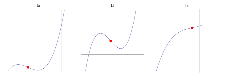
Figure 1: The value of $\tilde{A_{1}}$ and of $\tilde{A_{2}}$ is positive

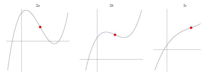
Figure 2: The value of $\tilde{A_{1}}$ is positive and of $\tilde{A_{2}}$ is negative

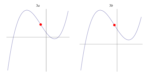
Figure 3: The value of $\tilde{A_{1}}$ is negative and of $\tilde{A_{2}}$ is positive

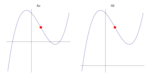
Figure 4: The value of $\tilde{A_{1}}$ is negative and of $\tilde{A_{2}}$ is negative

Figures 1, 2, 3, 4 show that there are several cases when delay does not destabilize the system for any $\alpha$, for example if $\tilde{A_{2}}>0$, $\tilde{A_{1}}>0$, and the cases when $H(\alpha)$ has a single real root only. Furthermore, if $\alpha$ increases through a limit, namely if $\frac{1}{\alpha}$ is small, ”measure of the influence of the past” is small then the system (10) has a locally asymptotically stable equilibrium point $E^{*}_{d}$. This situation corresponds to our expectation and it is similar as it was in the $2$-dimensional case, see in [1].
Now we can formulate our main result. We will give appropriate conditions that can easily be checked in order to satisfy $\tilde{A_{2}}>0$, $\tilde{A_{1}}>0$.

Theorem 2.2.

If matrix $A_{d}$ given by (18) in case of $n=2$ satisfies conditions (15),(16),(17) for $i=1,2$ (has the same sign pattern as (19)) and the following two conditions also hold

$$a_{11}^{2}>a_{33}^{2}>-a_{13}a_{34},$$ (23)

$$a_{11}^{2}>a_{22}^{2}>-a_{12}a_{24}$$ (24)

then $A_{d}$ is stable and $E^{*}_{d}$ is an asymptotically stable equilibrium point of the delayed system (10) in case of $n=2$ for any $\alpha>0$.

Proof.

Under the conditions of the theorem we can decompose the expression of $\tilde{A_{1}}$ into the following positive terms:

$$\tilde{A_{1}} = (a_{22}^{2}+a_{12}a_{24})(-a_{33}^{3}-a_{11}a_{33}^{2}-a_{11}a_{22}a_{33})+(a_{33}^{2}+a_{13}a_{34})(-a_{22}^{3}-a_{11}a_{22}^{2}-a_{11}a_{22}a_{33})$$

$$+ (a_{11}^{2}-a_{33}^{2})(a_{22}a_{12}a_{24})+(a_{11}^{2}-a_{22}^{2})(a_{33}a_{13}a_{34})$$

$$+ (-a_{11}^{3}a_{22}^{2}-a_{11}^{2}a_{22}^{3}+a_{11}a_{22}^{2}a_{12}a_{24}-2a_{11}^{3}a_{22}a_{33}-4a_{11}^{2}a_{22}^{2}a_{33}-a_{11}a_{22}^{3}a_{33}$$

$$-a_{11}^{3}a_{33}^{2}-4a_{11}^{2}a_{22}a_{33}^{2}-2a_{11}a_{22}^{2}a_{33}^{2}-a_{11}^{2}a_{33}^{3}-a_{11}a_{22}a_{33}^{3}+a_{11}a_{33}^{2}a_{13}a_{34})$$

$$> 0$$

and similarly for the expression of $\tilde{A_{2}}:$

$$\tilde{A_{2}} = (a_{22}^{2}+a_{12}a_{24})(a_{11}a_{33}+a_{22}a_{33}+a_{33}^{2}-a_{12}a_{24})+(a_{33}^{2}+a_{13}a_{34})(a_{11}a_{22}+a_{22}a_{33}+a_{22}^{2}-a_{13}a_{34})$$

$$+ (-a_{11}^{2}a_{12}a_{24}-a_{11}^{2}a_{13}a_{34}-2a_{12}a_{24}a_{13}a_{34})$$

$$+ (a_{11}^{3}a_{22}+2a_{11}^{2}a_{22}^{2}+a_{11}a_{22}^{3}-a_{11}a_{22}a_{12}a_{24}+a_{11}^{3}a_{33}+4a_{11}^{2}a_{22}a_{33}+$$

$$3a_{11}a_{22}^{2}a_{33}+2a_{11}^{2}a_{33}^{2}+3a_{11}a_{22}a_{33}^{2}+a_{11}a_{33}^{3}-a_{11}a_{33}a_{13}a_{34})$$

$$> (a_{22}^{2}+a_{12}a_{24})(a_{11}a_{33}+a_{22}a_{33}+a_{33}^{2}-a_{12}a_{24})+(a_{33}^{2}+a_{13}a_{34})(a_{11}a_{22}+a_{22}a_{33}+a_{22}^{2}-a_{13}a_{34})$$

$$+ (-a_{33}^{2}a_{12}a_{24}-a_{22}^{2}a_{13}a_{34}-2a_{12}a_{24}a_{13}a_{34})$$

$$+ (a_{11}^{3}a_{22}+2a_{11}^{2}a_{22}^{2}+a_{11}a_{22}^{3}-a_{11}a_{22}a_{12}a_{24}+a_{11}^{3}a_{33}+4a_{11}^{2}a_{22}a_{33}+$$

$$3a_{11}a_{22}^{2}a_{33}+2a_{11}^{2}a_{33}^{2}+3a_{11}a_{22}a_{33}^{2}+a_{11}a_{33}^{3}-a_{11}a_{33}a_{13}a_{34})$$

$$= (a_{22}^{2}+a_{12}a_{24})(a_{11}a_{33}+a_{22}a_{33}+a_{33}^{2}-a_{12}a_{24})+(a_{33}^{2}+a_{13}a_{34})(a_{11}a_{22}+a_{22}a_{33}+a_{22}^{2}-a_{13}a_{34})$$

$$+ (-a_{12}a_{24}(a_{33}^{2}+a_{13}a_{34})-a_{13}a_{34}(a_{22}^{2}+a_{12}a_{24}))$$

$$+ (a_{11}^{3}a_{22}+2a_{11}^{2}a_{22}^{2}+a_{11}a_{22}^{3}-a_{11}a_{22}a_{12}a_{24}+a_{11}^{3}a_{33}+4a_{11}^{2}a_{22}a_{33}+$$

$$3a_{11}a_{22}^{2}a_{33}+2a_{11}^{2}a_{33}^{2}+3a_{11}a_{22}a_{33}^{2}+a_{11}a_{33}^{3}-a_{11}a_{33}a_{13}a_{34})$$

$$> 0$$

∎

This theorem means that in case of a sign-stable interaction matrix (12) there are many cases when delay does not destabilize the system. By Theorem 2.1, if $a_{11}\leq 0$ (given by (13)) and if conditions (16), (17) are also satisfied then (12) is sign-stable. This is the two-dimensional situation modeled by Farkas and Cavani in [1] when the equilibrium point lies on the descending branch of the prey nullcline. That is the case when $E^{*}$ lies outside the Allée-effect zone – here the effect of overcrowding is already felt. Any further increase in prey quantity must be counterbalanced by a decrease in predator quantity, see in [4]. On the other hand, in the Allée-effect zone prey is scarce and an increase in prey quantity is beneficial for the growth rate of prey, see in [4]. Let us introduce the vector

$$F(x,y_{1},y_{2},\dots,y_{n})=\left[\begin{array}[]{c}rxg(x,K)-\displaystyle\sum_{i=1}^{n}y_{i}p_{i}\left(\frac{y_{i}}{x}\right)\\ y_{1}p_{1}\displaystyle\left(\frac{y_{1}}{x}\right)-d_{1}y_{1}\\ \vdots\\ y_{n}p_{n}\displaystyle\left(\frac{y_{n}}{x}\right)-d_{n}y_{n}\end{array}\right].$$ (25)

Vector (25) has two rows $F_{1}$ and $F_{2}$ in the two-dimensional case. Suppose that any predator quantity growth will decrease the growth rate of prey, namely $F^{\prime}_{1_{y_{1}}}<0$. Some typical reasonable forms of $F_{1}(x,y_{1})=0$ zero isoclines applicable to most species in case of ratio-dependence are shown in Figure 5. We can see that $F^{\prime}_{1_{x}}>0$, thus $a_{11}>0$ in the Allée-effect zone modelled by the increasing branch of the function in the third graph.

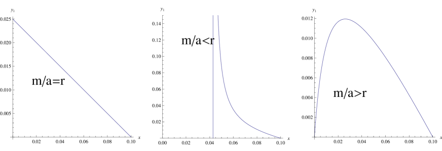
Figure 5: Typical nullclines of prey in case of 2–dimension

In case of our model we keep this meaning of the Allée-effect zone, and we say we are outside of the Allée-effect zone if in order to keep the prey growth rate zero the increase of prey can be counterbalanced by the decrease of the whole quantities of the different predators. Let us consider the higher dimensional cases. Now the function $F$ given by (25) has $n+1$ rows $F_{i}$, $i=1,2,\dots,n+1$. Suppose that any predator quantity growth will decrease the growth rate of prey, namely $F^{\prime}_{1_{y_{i}}}<0$, $i=1,2,\dots,n$. In the three dimensional case a typical onion-like prey zero isocline surface of $F_{1}(x,y_{1},y_{2})=0$ is shown in Figure 2.4.2 in [4] page 44 without ratio-dependence. Inside the onion-like surface $F_{1}>0$ while outside $F_{1}<0$. Function $F$ is increasing as we cross the surface inwards and therefore its gradient points inward. Therefore if the equilibrium point is on the eastern hemisphere of this onion then $F^{\prime}_{1_{x}}<0$, thus, $a_{11}<0$ and on the western hemisphere of the onion $F^{\prime}_{1_{x}}>0$, thus, $a_{11}>0$ and we can see that $F^{\prime}_{1_{x}}>0$, thus $a_{11}>0$ in the Allée-effect zone. The onion is similar to this in case of ratio-dependence shown in Figures 6, 7, 8.

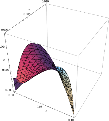
Figure 6: Typical zero-cline of prey in case of $r=3$ in 3–dimensions ($r=3,\;K=0.1,\;m_{1}=16,\;a_{1}=4,\;m_{2}=18,\;a_{2}=2$)

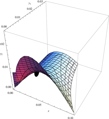
Figure 7: Typical zero-cline of prey in case of $r=7$ in 3–dimensions ($r=7,\;K=0.1,\;m_{1}=16,\;a_{1}=4,\;m_{2}=18,\;a_{2}=2$)

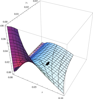
Figure 8: Typical zero-cline of prey in case of $r=10$ in 3–dimensions ($r=10,\;K=0.1,\;m_{1}=16,\;a_{1}=4,\;m_{2}=18,\;a_{2}=2$)

If $F^{\prime}_{1_{y_{i}}}<0$ (namely $y_{i}$ is predator of $x$) then $a_{11}>0$ holds also in higher dimension in the Allée-effect zone. To see this, let us consider $F_{1}(x,y_{1},\dots,y_{n})=rxg(x,K)-\displaystyle\sum_{i=1}^{n}y_{i}p_{i}\left(\frac{y_{i}}{x}\right)$ and surface $F_{1}(x,y_{1},\dots,y_{n})=0$, which is the prey zero isocline surface. Let be $E^{1}=(x^{1},y_{1}^{1},\dots,y_{n}^{1}),\;\;E^{2}=(x^{2},y_{1}^{2},\dots,y_{n}^{2})$ two different points in the Allée-effect zone on the prey isocline surface, where $x^{1}<x^{2},\;\;y_{i}^{1}<y_{i}^{2},\;\;,i=1,\dots,n$.

$$0 = F_{1}(x^{2},y_{1}^{2},\dots,y_{n}^{2})-F_{1}(x^{1},y_{1}^{1},\dots,y_{n}^{1})$$

$$= \{F_{1}(x^{2},y_{1}^{2},\dots,y_{n}^{2})-F_{1}(x^{2},y_{1}^{1},y_{2}^{2}\dots,y_{n}^{2})\}$$

$$+ \{F_{1}(x^{2},y_{1}^{1},y_{2}^{2}\dots,y_{n}^{2})-F_{1}(x^{2},y_{1}^{1},y_{2}^{1},y_{3}^{2},y_{4}^{2},\dots,y_{n}^{2})\}$$

$$+ \{F_{1}(x^{2},y_{1}^{1},y_{2}^{1},y_{3}^{2},y_{4}^{2},\dots,y_{n}^{2})-F_{1}(x^{2},y_{1}^{1},y_{2}^{1},y_{3}^{1},y_{4}^{2},\dots,y_{n}^{2})\}+\dots$$

$$+ \{F_{1}(x^{2},y_{1}^{1},y_{2}^{1},y_{3}^{1},\dots,y_{n-1}^{1},y_{n}^{2})-F_{1}(x^{2},y_{1}^{1},y_{2}^{1},y_{3}^{1},\dots,y_{n-1}^{1},y_{n}^{1})\}$$

$$+ \{F_{1}(x^{2},y_{1}^{1},y_{2}^{1},y_{3}^{1},\dots,y_{n}^{1})-F_{1}(x^{1},y_{1}^{1},\dots,y_{n}^{1})\}.$$

Expressions in the brackets are negative except the last bracket because of $F^{\prime}_{y_{i}}<0$, thus $F_{x}>0$ must hold.
It is reasonable to say that $E^{*}$ lies outside the Allée-effect zone if $a_{11}<0$ and $E^{*}$ lies in the Allée-effect zone if $a_{11}>0$.

Remark 2.1.

Theorem 2.2 means, if $E^{*}$ lies outside the Allée-effect zone then delay does not change the stability behaviour of the system in this special case.

This remark is a direct generalization of Case 1 of [1] on page 226.
The meaning of conditions (23), (24) are the following:
Conditions $a_{11}^{2}>a_{33}^{2}$, $a_{11}^{2}>a_{22}^{2}$ mean that intraspecific competition in prey species is greater than intraspecific competition in predators species.
The meaning of conditions $a_{33}^{2}>-a_{13}a_{34}$, $a_{22}^{2}>-a_{12}a_{24}$ is in connection with the phenomenon of their consume strategy, namely do they try to ensure their survival by having a relatively high or low growth rate and are able or not to raise their offspring on a scarce supply of food. We will discuss this very interesting meaning of conditions (23), (24) in case of (3) and (4) or (5) in the following section.

2.2 Strategies

The condition $a_{11}\leq 0$ can be ensured by a relative high intrinsic growth rate $r$ of prey. This means that there is enough food for predators in order to reproduce well. If this fact is valid in a long term then we expect even more that a predator species has an advantage that need more food and has a high growth rate. The parameter $a_{i}>0$ is the half saturation constant of predator $i$. This means that when the quantity of prey reaches value $a_{i}$ then the per capita birth rate of predator $i$ reaches half of the maximal birth rate, as one can see in case of a simple Holling model where $p_{i}(x,a_{i})=m_{i}\frac{x}{a_{i}+x}$, $m_{i}$ is ”the maximal birth rate” of the $i$-th predator, and $p_{i}(a_{i},a_{i})=\frac{m_{i}}{2}$. In case of ratio-dependent models parameter $a_{i}$ has a similar meaning, namely the greater $a_{i}$ is the more food is needed for predator $i$. To see this let us consider the ratio-dependent Holling function, given by (4). In this case at a fixed value of $y_{i}$, $p_{i}(x,y_{i},a_{i})=\frac{m_{i}}{2}$ if $x=a_{i}y_{i}$. Similarly in case of the ratio-dependent Ivlev function, given by (5) at a fixed value of $y_{i}$, $p_{i}(x,y_{i},a_{i})=\frac{m_{i}}{2}$ if $x=a_{i}y_{i}\ln 2$. Thus, a predator with a big half saturation constant can be considered as an r-strategist and with a lower one as a K-strategist. See in [6], [4]. Thus, we expect that the parameters $a_{i}$ cannot be arbitrary small, because the mentioned effect is stronger in that case when the time average of prey quantity over the past has the same influence on the present growth rates of different predators. The following theorems express this situation.

Theorem 2.3.

Let matrix $A_{d}$ be given by (18) in case of $n=2$ satisfying conditions (15),(16),(17) for $i=1,2$ (i.e. $A_{d}$ has the same sign pattern as (19)) and the function $g$, $p_{i}$ are given by (3), (4), respectively. If $a_{i}>1$ for $i=1,2$ then conditions (23), (24) are satisfied.

Proof.

Calculate $a_{33}^{2}>-a_{13}a_{34}$, $a_{22}^{2}>-a_{12}a_{24}$ by substituting (3), (4) and the statement follows. ∎

Theorem 2.4.

Let matrix $A_{d}$ be given by (18) in case of $n=2$ satisfying conditions (15),(16),(17) for $i=1,2$ (i.e. $A_{d}$ has the same sign pattern as (19)) and the function $g$, $p_{i}$ are given by (3), (5), respectively. If $a_{i}>\frac{1}{2}$ for $i=1,2$ then conditions (23), (24) are satisfied.

Proof.

Calculate $a_{33}^{2}>-a_{13}a_{34}$, $a_{22}^{2}>-a_{12}a_{24}$ by substituting (3), (5) we get:

$$a_{i}>\frac{\frac{d_{i}}{m_{i}}-\frac{m_{i}-d_{i}}{m_{i}}\ln\frac{m_{i}}{m_{i}-d_{i}}}{(\ln\frac{m_{i}}{m_{i}-d_{i}})^{2}}.$$ (26)

Let us denote $x=\frac{m_{i}}{m_{i}-d_{i}},\;\;x>1.$ Thus,

$$a_{i}(x)=\frac{1-\frac{1}{x}-\frac{1}{x}\ln x}{(\ln x)^{2}},$$

where $\lim_{x\rightarrow 1+0}a_{i}(x)=\frac{1}{2}$ and $a_{i}(x)$ is monotone decreasing for $x>1$ because its derivative is: $a_{i}(x)^{\prime}=\frac{\frac{1}{x^{2}}((\ln x)^{2}-2x+2+2\ln x)}{(\ln x)^{3}}$ and the numerator is negative because it is zero if $x=1$ and the derivative of $((\ln x)^{2}-2x+2+2\ln x)$ is negative for $x<1$. Thus, the maximum of the righthand side of (26) is equal to $\frac{1}{2}$ and theorem holds. ∎

The meaning of Theorems 2.3, 2.4 corresponds to our expectation, namely in case of delayed models the advantage of the r-strategist can be seen over the K-strategist. This advantage is greater in case of a ratio-dependent Holling model than in case of a ratio-dependent Ivlev model.

2.3 One prey, $n$ predators with delay

Now let the number of predators $n$ be an arbitrary positive integer and let us consider system (1) with its coefficient matrix given by (12). Let us denote the entries of (12) by $a_{ij},$ thus

$$A=\left[\begin{array}[]{llllll}a_{11}&a_{12}&\dots&\dots&\dots&a_{1n}\\ a_{21}&a_{22}&0&\dots&\dots&0\\ a_{31}&0&a_{33}&\dots&\dots&0\\ \vdots&\vdots&\vdots&\vdots&\vdots&0\\ a_{n-1,1}&0&0&\dots&a_{n-1,n-1}&0\\ a_{n1}&0&0&\dots&0&a_{nn}\end{array}\right].$$ (33)

If we modify system (1) with delay we get system (10) which, after linearization has the coefficient matrix given by (18). We have seen that (18) can be obtained from the entries of $A$ as follows:

$$A_{d}=\left[\begin{array}[]{llllll}a_{11}&a_{12}&a_{13}&\dots&a_{1n}&0\\ 0&a_{22}&0&\dots&0&a_{21}\\ 0&0&a_{33}&\dots&0&a_{31}\\ \vdots&\vdots&\vdots&\vdots&\vdots&\vdots\\ 0&0&0&\dots&a_{nn}&a_{n1}\\ \alpha&0&0&\dots&0&-\alpha\end{array}\right].$$ (40)

Theorem 2.5.

Let matrix $A_{d}$ be given by (18) for arbitrary positive integer $n,$ and suppose it satisfies conditions (16) and (17) for all $i=1,2,\dots,n;$ and let $a_{11}<0.$ If $\alpha$ is small enough or large enough then $A_{d}$ is stable, and $E_{d}^{*}$ is an asymptotically stable equilibrium state of the delayed system (10).

Proof.

Let us consider the characteristic polynomial $\mathcal{D}(\lambda):=\det(A_{d}-\lambda E)$ of (40). Let us denote column $i$ of matrix $A_{d}$ by $\mathbf{c}_{i},$ $(i=1,2,\dots,n)$ and let us make the following column operations: first $\mathbf{c}_{1}\Longrightarrow\mathbf{c}_{1}+\mathbf{c}_{n+1},$ then $\mathbf{c}_{n+1}\Longrightarrow\mathbf{c}_{n+1}-\mathbf{c}_{1}.$ Now we get

$$\det(A_{d}-\lambda E)=\left[\begin{array}[]{rrrrr}a_{11}-\lambda&a_{12}&\dots&a_{1n}&-(a_{11}-\lambda)\\ a_{21}&a_{22}-\lambda&\dots&0&0\\ a_{31}&0&a_{33}-\lambda&0\\ \dots&\dots&\ddots&\dots&\dots\\ a_{n1}&\dots&\dots&a_{nn}-\lambda&0\\ -\lambda&0&\dots&0&-\alpha\end{array}\right].$$ (41)

Let us make the following partition of this determinant:

$$\det(A_{d}-\lambda E)=\det\left[\begin{array}[]{ccccccc}&&A-\lambda E&&&|&\left[\begin{array}[]{c}-(a_{11}-\lambda)\\ 0\\ \vdots\\ 0\end{array}\right]\\ -&-&-&-&-&|&---\\ -\lambda&0&\dots&\dots&0&|&-\alpha\end{array}\right]=\det\left[\begin{array}[]{cc}A-\lambda E&B\\ C&D\end{array}\right].$$ (42)

Applying the Schur theorem [9, Theorem 3.1.1] we get:

$$\det(A_{d}-\lambda E)=\det(A-\lambda E)\det(A_{d}-\lambda E|A-\lambda E),$$

where $(A_{d}-\lambda E|A-\lambda E)$ is the Schur-complement of $A-\lambda E$ in $A_{d}-\lambda E,$ namely $(A_{d}-\lambda E|A-\lambda E)=D-C(A-\lambda E)^{-1}B$ and suppose that $\lambda$ is not an eigenvalue of $A.$

$$(A_{d}-\lambda E|A-\lambda E) = D-C(A-\lambda E)^{-1}B$$ (48)

$$= -\alpha-[\begin{array}[]{cccc}-\lambda&0&\dots&0\end{array}](A-\lambda E)^{-1}\left[\begin{array}[]{c}-(a_{11}-\lambda)\\ 0\\ \vdots\\ 0\end{array}\right]$$

$$= -\alpha-\lambda(a_{11}-\lambda)A_{11}^{-1},$$ (49)

where $A_{11}^{-1}:=\frac{1}{\det(A-\lambda E)}(a_{22}-\lambda)\cdot\dots\cdot(a_{nn}-\lambda),$ thus,

$$\det(A_{d}-\lambda E|A-\lambda E)=-\alpha-\lambda\frac{(a_{11}-\lambda)\cdot\dots\cdot(a_{nn}-\lambda)}{\det(A-\lambda E)}.$$

We get the following relation (true for all $\lambda\in\mathbb{C}$)

$$\det(A_{d}-\lambda E) = -\alpha\det(A-\lambda E)-\lambda(a_{11}-\lambda)\cdot\dots\cdot(a_{nn}-\lambda)$$ (50)

$$= (-1)(\alpha\det(A-\lambda E)+\lambda\prod_{i=1}^{n}(a_{ii}-\lambda)).$$

Now we prove that the coefficients of this polynomial have the same sign, using the fact that $A$ being sign stable, hence the coefficients of $\det(A-\lambda E)$ have the same sign. Let us denote the coefficients of $\det(A-\lambda E)$ by $a_{i},$ namely:

$$\det(A-\lambda E)=(-\lambda)^{n}+a_{n-1}(-\lambda)^{n-1}+\dots+a_{0}.$$

Thus,

$$\det(A_{d}-\lambda E) = (-1)\{\alpha(-\lambda)^{n}+\alpha a_{n-1}(-\lambda)^{n-1}+\dots+\alpha a_{0}$$

$$+\lambda((-\lambda)^{n}+(a_{11}+\dots+a_{nn})(-\lambda)^{n-1}$$

$$+(a_{11}a_{22}+\dots+a_{n-1n-1}a_{nn})(-\lambda)^{n-2}$$

$$+\dots+(a_{11}a_{22}\cdot\dots\cdot a_{nn}))\}$$

$$= (-\lambda)^{n+1}+(a_{11}+\dots+a_{nn}-\alpha)(-\lambda)^{n}$$

$$+(a_{11}a_{22}+\dots+a_{n-1n-1}a_{nn}-\alpha a_{n-1})(-\lambda)^{n-1}$$

$$+\dots+(a_{11}a_{22}\cdot\dots\cdot a_{nn}-\alpha a_{1})(-\lambda)-\alpha a_{0}.$$

Since $\det(A-\lambda E)$ is a stable polynomial, hence if $n$ is even, then $a_{2k}$ is positive, and $a_{2k+1}$ is negative for all $k.$ Thus, the coefficients with even indices of $\det(A_{d}-\lambda E)$ are negative, and those with odd indices are positive, and all the coefficients of $(\lambda)^{j}\quad(j=0,1,\dots,n+1)$ in $\det(A_{d}-\lambda E)$ are negative.

For the case of $n$ odd we can repeat the above proof. Thus the necessary condition of stability of the polynomial $\det(A_{d}-\lambda E)$ holds.

This means that if $\det(A_{d}-\lambda E)$ is not a stable polynomial then it has to have a pair of complex conjugate roots with nonnegative real part.

Now let us consider the case when $\alpha$ is very large. Then the eigenvalues of $\det(A_{d}-\lambda E)$ are close to the eigenvalues of $A$ and there is a remaining root with an unknown sign. But this root should also be a negative real number, because it has no pair to be a member of a complex conjugate pair, and because the coefficients of the characteristic polynomial are positive. Thus, for sufficiently large $\alpha\gg 0$ the matrix $A_{d}$ is stable.

If $\alpha$ is very small then the eigenvalues of $\det(A_{d}-\lambda E)$ are close to the roots of $\lambda\prod_{i=1}^{n}(a_{ii}-\lambda)=0.$ It has $n$ negative real roots and one more root left with an unknown sign. And again, this should be a negative real number, because it has no pair to be a member of a complex conjugate pair, and because the coefficients of the characteristic polynomial are positive. Thus, for sufficiently small $\alpha\neq 0$ the matrix $A_{d}$ is stable. This completes the proof of the theorem. ∎

The meaning of this theorem is the following. If $\alpha$ is small then the measure of the influence of the past is large. In this case the equilibrium point $E_{d}^{*}$ is locally asymptotically stable.

If $\alpha$ is large then the measure of the influence of the past is small, the system’s behaviour is close to the behaviour of the system without delay, of which the equilibrium $E^{*}$ was stable. Thus, the results correspond to our expectations. But all these are true outside the Allée-effect zone, where the stability is stronger than inside.

2.4 Numerical examples

Example 2.1.

Let us consider a three dimensional Holling type ratio-dependent model with delay, namely $g$ is given by (3) and $p_{i}$ is given by (4). Let the constants be given as follows: $m_{1}=16,\;m_{2}=18,\;d_{1}=8,\;d_{2}=12,\;a_{1}=4,\;a_{2}=2,\;K=0.1.$ The equilibrium point of the system depending on $r$ is $E^{*}=\left(0.1(1-\frac{5}{r}),\frac{1}{40}(1-\frac{5}{r}),\frac{1}{40}(1-\frac{5}{r})\right).$ In this case the interaction matrix of the system without delay is given by:

$$A=\left[\begin{array}[]{ccc}8-r&-4&-8\\ 1&-4&0\\ 1&0&-4\end{array}\right].$$ (51)

The characteristic polynomial of $A$ is: $D(\lambda)=(-4-\lambda)\left(\lambda^{2}+(r-4)\lambda+4(r-5)\right).$ This is a stable polynomial for $r>5$ and $A$ is sign stable for $r\geq 8$ .
The equilibrium point of the delayed system depending on $r$ is

$${E_{d}}^{*}=\left(0.1(1-\frac{5}{r}),\frac{1}{40}(1-\frac{5}{r}),\frac{1}{40}(1-\frac{5}{r}),0.1(1-\frac{1}{r})\right).$$

The coefficient matrix of the delayed system linearized at ${E_{d}}^{*}$ is

$$A=\left[\begin{array}[]{cccc}8-r&-4&-8&0\\ 0&-4&0&1\\ 0&0&-4&1\\ \alpha&0&0&-\alpha\end{array}\right].$$ (52)

The characteristic polynomial of $A_{d}$ is: $D_{d}(\lambda)=(-4-\lambda)\left((8-r-\lambda)(-4-\lambda)(-\alpha-\lambda)-12\alpha\right).$

Let us check conditions (23), (24). It is easy to see that in case of $r>12$ these are satisfied. The conditions of Theorem 2.2 hold, ${E_{d}}^{*}$ is asymptotically stable. Time evolution of the species are shown on the left side of Fig. 9, whereas the right side shows the corresponding trajectory together with the equilibrium point.

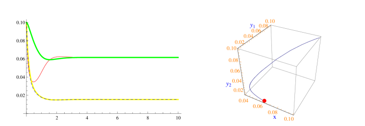
Figure 9: Left: Time evolution of the species in case of $r=13,\;\alpha=1$. Right: The trajectory tends to the asymptotically stable equilibrium point. ($x$ is red, $q$ is green, $y_{1}$ is dashed blue, $y_{2}$ is yellow.)

The form of (22) with $r=13$ is shown in Fig. 10. This corresponds to Fig. 1, case 1c.

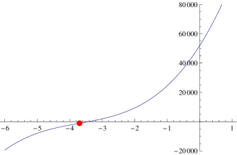
Figure 10: The function (22) with $r=13$

It is easy to see that the equilibrium point of the delay system remains asymptotically stable for any $\alpha>0.$ We note that in this case the equilibrium point is outside the Allée-effect zone, see Fig. 8.

If $12\geq r>5$ then conditions (23), (24) are not valid, and there are such cases when ${E_{d}}^{*}$ is stable and there are cases when it is unstable. Time evolution of the species are shown on the left side of Fig. 11, whereas the right side shows the corresponding trajectory together with the equilibrium point.

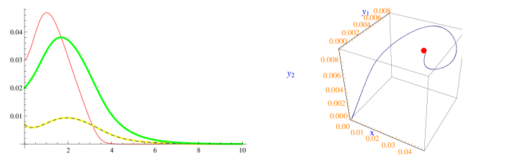
Figure 11: Left: Time evolution of the species in case of $r=7,\;\alpha=1$. Right: The trajectory leaves the neighbourhood of the unstable equilibrium point. ($x$ is red, $q$ is green, $y_{1}$ is dashed blue, $y_{2}$ is yellow.)

The form of (22) with $r=7$ is shown in Fig. 12.

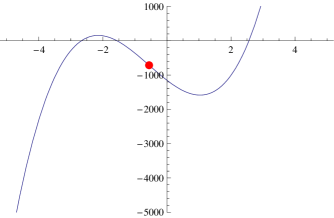
Figure 12: The function (22) with $r=7$

It is easy to see that there are values of $\alpha$ for which $H(\alpha)<0,$ thus, the equilibrium point of the delay system is unstable, and also values for which $H(\alpha)>0,$ thus, the equilibrium point of the delay system is asymptotically stable. We note that in this case the equilibrium point is inside the Allée-effect zone, see Fig. 7.

Of course this study is not complete. There are many interesting trajectories, periodic orbits, see e. g. Fig. 13, 14.

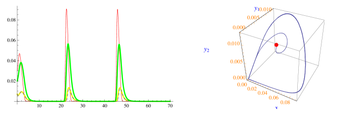
Figure 13: Left: Time evolution of the species in case of $r=7,\;\alpha=1$. The solution seems to be periodic at first sight. (The reason of this phenomenon may also be numerical errors.) Right: The corresponding trajectory. ($x$ is red, $q$ is green, $y_{1}$ is dashed blue, $y_{2}$ is yellow.)

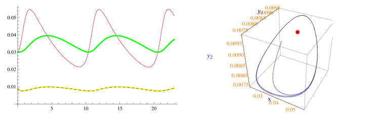
Figure 14: Left: Seemingly time periodic evolution of the species in case of $r=8,\;\alpha=0.2$. Right: The corresponding periodic orbit. ($x$ is red, $q$ is green, $y_{1}$ is dashed blue, $y_{2}$ is yellow.)

The interested reader can experiment with the parameters and initial conditions of the model using the Mathematica program on the page http://www.math.bme.hu/~jtoth.

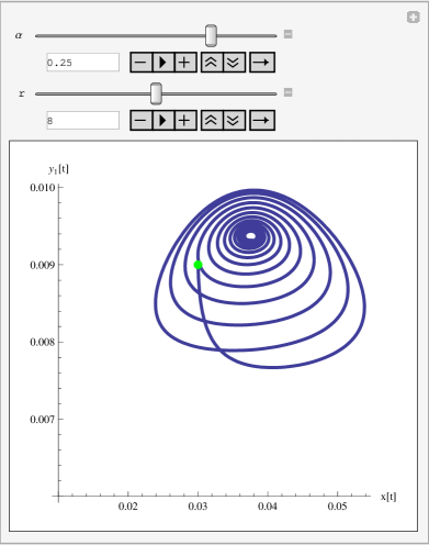
Figure 15: Snapshot of manipulation. $r=8$ and $\alpha=0.25.$

In case of an Ivlev model similar situations may occur.

Acknowledgement
This work is partly the generalization of a paper of Cavani and Farkas [1]. The first author was a student of the late Prof. Miklós Farkas of Budapest University of Technology and Economics. They worked together for more than twenty years. Prof. Miklós Farkas regrettably died on the 28th of August 2007. She is eternally thankful to him for his precious ideas and comments throughout so many years. The second author really regrets not having learned more from Professor Farkas. The authors are honored to have known him, and remember him with great fondness, love and gratitude.

The present work has partially been supported by the National Science Foundation, Hungary (K63066).

References

- [1] Cavani, M., Farkas, M.: Bifurcations in a Predator-Prey Model with Memory and Diffusion I: Andronov-Hopf Bifurcation, Acta Math. Hungar. 63 (3) (1994), 213–229.
- [2] Cushing, J.M.: Integodifferential Equations and Delay Models in Population Dynamics, Lect. Notes Biomath. 20 Springer (Berlin, 1977).
- [3] Farkas, M.: Periodic Motions, Springer-Verlag, Applied Mathematical Sciences 105 (1994)
- [4] Farkas, M. Dynamical Models in Biology, Academic Press, New York, 2001.
- [5] Jeffries, C., Klee, V., van den Driessche, P. Qualitative Stability of Linear Systems, Lin. Alg. and its Appl. 87 (1987) 1–48.
- [6] Kiss, K., Kovács, S.: Qualitative behaviour of n-dimensional ratio-dependent predator-prey systems, Appl. Math. Comput. 199 (2) (2008), 535–546. doi: 10.1016/j.amc.2007.10.019
- [7] MacDonald, N.: Time delay in prey-predator models, II. Bifurcation theory, Math. Biosci. 33 (1977), 226–234.
- [8] Lizana, M., Marín, J.: On Predator-Prey System with Diffusion and Delay, Discrete and Continuous Dynamical Systems - Series B 6 (6) (2006), 1321–1338.
- [9] Prasolov, V. V.: Problems and Theorems in Linear Algebra, Translations of Mathematical Monographs, vol. 134, American Mathematical Society, Providence, RI, 1994.