Abstract: In this contribution, we study a single Cooper pair box interacts with a single cavity mode. We show the roles played by the detuning parameters and charged capacities on the degree of entanglement. For large values of the detuning parameter the survival entanglement increases on the expanse of the degree of entanglement. We generate a maximum entangled state and use it to perform the original teleportation protocol. The fidelity of the teleportated state is increased with decreasing the detuning parameter and the number of photon inside the cavity.

Keywords: Charged Qubit, Entanglement and Teleportation. 

1 Introduction

Several schemes have been proposed for implementing quantum computer hardware in solid state quantum electronics. These schemes use electric charge [1], magnetic flux[2] and superconducting phase [3] and electron spin [4]. The basic element of the quantum information is the quantum bit (qubit) which is considered as a two level system. Consequently, most of the research concentrate to generate entanglement between two level systems [5]. Among these systems, the Cooper charged pairs, due to its properties as a two -level quantum system, which makes it a candidate as a qubit in a quantum computer [6, 7]. So there are a lot of studies have been done on these particle from different points of view in the context of quantum information. One of the most important tasks in the context of quantum information, is the quantum teleportation, which emerges from the quantum entanglement, and since the first quantum teleportation protocol was introduced by Bennett et al [8], there are a lot of attentions has been payed to it [9, 10, 11].

In our contribution, we consider a system consists of a single Cooper pair interactsa with a cavity mode. The separability problem is investigated, where the intervals of time in which the generated state is entangled or separable are determined. On the other hand under a specific circumstance one can use this system to generated a maximum entangled state. Finally we use the generated entangled state to perform the quantum teleportation.

The paper is organized as follows: The description of the system and its solution are introduced in Sec.$2$. In Sec.$3$, the separability problem and the degree of entanglement contained in the generated entangled state are investigated. Sec.$4$, is devoted to study the effect of the field and the charged qubit parameters on the phenomena of entanglement and quantum teleportation.

2 The Model and its evolvement

The single superconducting charged qubit consists of a small superconducting island with Cooper pair charge $Q$. This island connected by two identical Josephson junctions, with capacitance $C_{j}$ and Josephson coupling energy $E_{j}$, to a superconducting electrode [12, 14]. This system is described by the Hamiltonian,

$$H_{s}=4E_{c}(n-n_{g})^{2}-E_{j}\cos\phi,$$ (1)

where $E_{c}=e^{2}/2(C_{g}+C_{j})$ is the charging energy, $E_{j}=\hbar I_{c}/2e$ is the Josephson coupling energy, $e$ is the charge of the electron, $n_{g}=C_{g}V_{g}/2e$ is the dimensionless gate charge, $C_{g}$ is the gate capacitance, $v_{g}$ is controllable gate voltage, $n$ is number operator of excess cooper pair on the island and $\phi$ is phase operator [12].

The Hamiltonian of the system (1) can be simplified to a very simple form, if the Josephon coupling energy $E_{j}$ is much smaller than the charging energy i.e $E_{j}<<E_{c}$. In this case, the Hamiltonian of the system can be parameterized by the number of Cooper pairs $n$ on the island. If the temperature is low enough, the system can be reduced to two-state system (qubit) controlled by [13, 15],

$$H_{s}=-\frac{1}{2}B_{z}\sigma_{z}-\frac{1}{2}B_{x}\sigma_{x},$$ (2)

where $B_{z}=E_{cl}(1-2n_{j})$, $E_{cl}$ is the electric energy and $B_{x}=E_{j}$ and $\sigma_{z}$, $\sigma_{z}$ are Pauli matrices. This Cooper pair can be viewed as an atoms with large dipole moment coupled to microwave frequency photons in a quasi-one-dimensional transmission line cavity (a coplanar waveguide resonator). The combined Hamiltonian for qubit and transmission line cavity is given by,

$$H=\omega a^{\dagger}a+\omega_{c}\sigma_{z}-\lambda(\mu-\cos\theta\sigma_{z}+\sin\theta\sigma_{x})(a^{\dagger}+a),$$ (3)

where $\omega$ is the cavity resonance frequency, $\omega_{c}=\sqrt{E^{2}_{j}+[4E_{c}(1-2n_{g})]^{2}}$ is the transition frequency of the Cooper pair qubit, $\sigma_{z}$ and $\sigma_{x}$ are Pauli matrices, $\lambda=\frac{\sqrt{C_{j}}}{C_{g}+C_{j}}\sqrt{\frac{e^{2}\omega}{2\hbar}}$, is coupling strength of resonator to the cooper pair qubit, $\mu=1-n_{g}$, $\theta=arctan\{\frac{E_{j}}{E_{c}(1-2n_{g})}\}$, is the mixing angle.

Assume that we consider the charge degeneracy point, i.e $n_{g}=\frac{1}{2}$ and the radiation quantized field is weak. In this case we can neglect the fast oscillation by using the rotating wave approximation. Then the Hamiltonian (3) takes the form

$$H=\omega a^{\dagger}a+\frac{1}{2}\omega_{c}\sigma_{z}-\lambda(a^{\dagger}\sigma_{-}+\sigma_{+}a),$$ (4)

where $\sigma_{+}$ and $\sigma_{-}$ are the rasing and lowering operators such that $[\sigma_{+},\sigma_{-}]=\sigma_{z}$.

To investigate the dynamics of the total system (cooper pair box and the filed), let us consider that the charged qubit prior to the interaction, to be prepared in a superposition of its excited and ground state, i.e $\bigl{|}\psi_{c}(0)\bigr{\rangle}=\alpha\bigl{|}g\bigr{\rangle}+\beta\bigl{|}e\bigr{\rangle}$, and the filed is prepared in the number state $\bigl{|}\psi_{f}(0)\bigr{\rangle}=\bigl{|}n\bigr{\rangle}$. The time development of the state vector $\bigl{|}\psi(t)\bigr{\rangle}$ of the system is postulated to be determined by Schrödinger equation

$$i\hbar\frac{d}{dt}\bigl{|}\psi(t)\bigr{\rangle}=H\bigl{|}\psi(t)\bigr{\rangle}$$ (5)

The solution of Eq.(5) can be written as $\bigl{|}\psi(t)\bigr{\rangle}=U(t)\bigl{|}\psi(0)\bigr{\rangle}$, where $U(t)$ is the unitary operator. In an explicit for the evolvement of the density operator $\bigl{|}\psi(t)\bigr{\rangle}\bigl{\langle}\psi(t)\bigr{|}$ is given by

$$\rho(t) = A\Bigl{(}|\alpha|^{2}\bigl{|}g,n\bigr{\rangle}\bigl{\langle}g,n\bigr{|}+|\beta|^{2}\bigl{|}e,n\bigr{\rangle}\bigl{\langle}e,n\bigr{|}\Bigr{)}+B\alpha\beta^{*}\bigl{|}g,n\bigr{\rangle}\bigl{\langle}e,n\bigr{|}+B^{*}\alpha^{*}\beta\bigl{|}e,n\bigr{\rangle}\bigl{\langle}g,n\bigr{|}$$ (6)

$$+ iC\sqrt{n+1}(\alpha\beta^{*}\bigl{|}g,n\bigr{\rangle}\bigl{\langle}g,n+1\bigr{|}+\beta\alpha^{*}\bigl{|}g,n+1\bigr{\rangle}\bigl{\langle}g,n\bigr{|}\Bigr{)}$$

$$- iC\Bigl{(}\sqrt{n+1}|\beta|^{2}\bigl{|}e,n\bigr{\rangle}\bigl{\langle}g,n-1\bigr{|}+\sqrt{n}\beta\alpha^{*}\bigl{|}e,n\bigr{\rangle}\bigl{\langle}e,n-1\bigr{|}\Bigr{)}$$

$$+ i\eta C^{*}\Big{(}\sqrt{n+1}|\beta|^{2}\bigl{|}g,n+1\bigr{\rangle}\bigl{\langle}e,n\bigr{|}-\sqrt{n}|\alpha|^{2}\bigl{|}g,n\bigr{\rangle}\bigl{\langle}e,n-1\bigr{|}\Big{)}$$

$$+ \eta^{2}S^{2}_{n}\sqrt{n}\sqrt{n+1}\Bigl{(}\beta\alpha^{*}\bigl{|}g,n+1\bigr{\rangle}\bigl{\langle}e,n-1\bigr{|}+\alpha\beta^{*}\bigl{|}e,n-1\bigr{\rangle}\bigl{\langle}g,n+1\bigr{|}\Bigr{)}$$

$$+ S^{2}_{n}\Bigl{(}n|\alpha|^{2}\bigl{|}e,n-1\bigr{\rangle}\bigl{\langle}e,n-1\bigr{|}+(n+1)|\beta|^{2}\bigl{|}g,n+1\bigr{\rangle}\bigl{\langle}g,n+1\bigr{|}\Bigr{)}$$

$$+ i\sqrt{n}S_{n}\Bigl{(}|\alpha|^{2}C\bigl{|}e,n-1\bigr{\rangle}\bigl{\langle}g,n\bigr{|}+\alpha\beta^{*}C^{*}\bigl{|}e,n-1\bigr{\rangle}\bigl{\langle}e,n\bigr{|}\Bigr{)}$$

where

$$A = C^{2}_{n+1}+\frac{\Delta^{2}}{4}S^{2}_{n+1},~{}\quad B=C^{2}_{n+1}-\frac{\Delta^{2}}{4}S^{2}_{n+1}-i\Delta S_{n+1}C_{n+1}$$

$$C = iS_{n}(C_{n+1}+\frac{i\Delta}{2}S_{n+1}),~{}\quad C_{n}=\cos{(\gamma\mu_{n}\tau)},\quad S_{n}=\frac{\sin(\gamma\mu_{n}\tau)}{\mu_{n}},$$

$$\gamma = \frac{\sqrt{C_{j}}}{C_{g}+C_{j}},\quad\tau=\sqrt{\frac{e^{2}\omega}{2\bar{h}}}t,\quad\mbox{ is the scaled time}$$ (7)

with $\mu_{n}=\sqrt{\frac{\Delta^{2}}{4}+\lambda n}$, $\Delta=E_{j}-\omega$ is the detuning between the Josephson energy and the cavity field frequency .

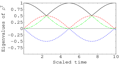
Figure 1: The behavior of the eigenvalues of the partial transpose $\rho^{T}$ is shown in Figs.$(a,b)$. The populations are shown in Fig.$(c,d)$ and the degree of entanglement is plotted in Figs.$(e,f)$. We assume $n=1,C_{jg}=\frac{5}{2}$ and $\Delta=0$ for Figs.$(a,c,e)$ while for Figs.$(b,d,f)$, $\Delta=1$.

3 Degree of entanglement

In this section, we study the behavior of the output state (6) from the separability point of view. To achieve this task, we plot time evolution of the the eigenvalues of the partial transpose eigenvalues of the output density operator $\rho^{T_{2}}$ [16, 17]. Also we investigate time development of the occupation probabilities and the degree of entanglement which contained in the output state. There are different measures known for quantifying the degree of entanglement in a bipartite system, such as the entanglement of formation [18, 19], entanglement of distillation [20], negativity [21].

In our calculations we consider the concurrence as a measure of the degree of entanglement. For two qubits, the concurrence is calculated in terms of the eigenvalues $\eta_{1},\eta_{2},\eta_{3}$ and $\eta_{4}$ of the matrix $R=\rho\sigma_{y}\otimes\sigma_{y}\rho^{*}\sigma_{y}\otimes\sigma_{y}.$ It is given by

$$\mathcal{C}=max\{0,\eta_{1}-\eta_{2}-\eta_{3}-\eta_{4}\},\mbox{where}~{}\eta_{1}\geq\eta_{2}\geq\eta_{3}\geq\eta_{4}.$$ (8)

For maximally entangled states concurrence is $1$ while $\mathcal{C}=0$ for separable states[20].

In the first example, we assume that the Cooper-pair box is initially prepared in the ground state and the field is prepared in the Fock state, i.e the initial state of the system is given by $\bigl{|}g,n\bigr{\rangle}$. In Fig.(1), we investigate the effect of the detuning parameter on the behavior of the eigenvalues of the partial transpose of the density operator of the output state, the time evaluation of the occupation probabilities and the degree of entanglement. For these numerical calculations, we assume that the ratio between the Josephson junction capacity, $C_{j}$, and the gate capacity $C_{g}$, is defined by $C_{jg}=\frac{C_{j}}{C_{g}}=\frac{5}{2}$ and $n=1$. In Fig.$(1a)$, we see that as the interaction goes on, i.e the scaled time, $\tau>0$, there is only one negative eigenvalues and the rest are non-negative. According to the Peres-Horodecki criterion [16, 17], there is an entangled state is generated. As the time increases we see that at specific time $\tau\simeq 5$ all the eigenvalues are non-negative. This means that the entangled qubit turns into a product state (separable).

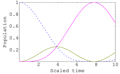
Figure 2: The same as Fig.$(1)$, but $\Delta=0,C_{jg}=\frac{2}{5}$.

In Fig.$(1c)$, we plot the occupation probabilities as functions of the scaled time. Note that the populations of the four states exist and it has different values for the diagonal occupations but for the off-diagonal occupations are completely coincide. For this reason an entangled state is generated as soon as the interaction starts. In this case the entangled state is

$$\rho=\kappa(\bigl{|}n,g\bigr{\rangle}\bigl{\langle}n-1,e\bigr{|}+\bigl{|}n-1,e\bigr{\rangle}\bigl{\langle}n,g\bigr{|})+\chi_{1}\bigl{|}n,g\bigr{\rangle}\bigl{\langle}n,g\bigr{|}+\chi_{2}\bigl{|}n-1,e\bigr{\rangle}\bigl{\langle}n-1,e\bigr{|},$$ (9)

where $\chi_{1}$ and $\chi_{2}$ are the probability to find the system in the state $\bigl{|}n,g\bigr{\rangle}\bigl{\langle}n,g\bigr{|}$ and $\bigl{|}n-1,e\bigr{\rangle}\bigl{\langle}n-1,e\bigr{|}$, respectively. In computational basis one can write it as $\rho=\kappa(\bigl{|}1,0\bigr{\rangle}\bigl{\langle}0,1\bigr{|}+\bigl{|}0,1\bigr{\rangle}\bigl{\langle}1,0\bigr{|})+\chi_{1}\bigl{|}1,0\bigr{\rangle}\bigl{\langle}1,0\bigr{|}+\chi_{2}\bigl{|}0,1\bigr{\rangle}\bigl{\langle}0,1\bigr{|}$. It is clear that the first bract is one type of Bell state $\bigl{|}\psi^{+}\bigr{\rangle}\bigl{\langle}\psi^{+}\bigr{|}$. However at $\tau\simeq 2.5$, the partially entangled state (9) becomes a maximum, where all the occupation probabilities have equal occupation probabilities at this point. This result is shown in from Fig.(1e), where we quantify the degree of entanglement by using the concurrence. From this figure, we can see that the degree of entanglement is increased as the time increased and reaches to the unity at $\tau\simeq 2.5$. Given enough time, the system will therefore reaches a state where all the occupation probabilities vanish. At specific time the system turns into a product state, this happens at $\tau\simeq 5$, (see Fig.$(1a)$). Also, on the left hand side of Fig.(1), we consider $\Delta=1$ and the other parameters are fixed, it is clear that as one increases $\Delta$, the system turns into a product round $\tau=5.4$. This means that the time of the entanglement survival increased. This phenomenon is clear shown by comparing Fig.(1a) and Fig.(1b). The behavior of the occupation probability is seen in Fig.(d), where there is no intersection point between the off diagonal occupation probabilities and the diagonal ones. So in this case one can not get a maximum entangled state. As time goes on the system becomes a separable at $\tau\simeq 5.4$, this result agrees with that depicted in Fig.$(1b)$. The amount of entanglement contained in the output state is shown in Fig.$(1f)$. From this figure, we can notice that the maximum entanglement is less than unity. So one can say that by increasing the detuning parameter, one can increase the survival time of entanglement on the expanse of the degree of entanglement.

The effect of the ratio of $C_{jg}$ is seen in Fig.(2), where we consider a small value of this ratio. We investigate the behavior of the occupation probabilities and the degree of entanglement only. It is clear that as one decreases $C_{jg}$, the first maximum entangled state is obtained round $\tau=4$. This means that for small ratio, one takes a larger time to generate maximum entangled state. Also, the point at which the system turns into a separable state is shifted. The degree of entanglement contained in this state is shown in Fig.(2b), where it has a unity value at the maximum entangled state. So, the ratio $C_{jg}$ has no effect on the value of the degree of entanglement.

Figure 3: The degree of entanglement for a system is initially prepared in the superposition state $\bigl{|}\psi_{0}\bigr{\rangle}=a\bigl{|}n,g\bigr{\rangle}+(1-a)\bigl{|}n,e\bigr{\rangle}$ with $a=0.5$, $C_{jg}=\frac{5}{2}$ and (a) $\Delta=0$, (b) $\Delta=1$.

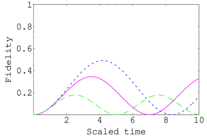
Figure 4: The Fidelity of the teleported state at Bob’s hand (a)For $C_{jg}=5$, number of photon, $n=1$ and dot, solid and the dashed curves for $\Delta=0.1,0.5$ and 1 respectively (b) The same as Fig.(a) but $\Delta=0.1$ and the dot, the solid and the dash curves for $C_{jg}=5/3,5/2$ and $5$ respectively.

Our second case, we assume that the Cooper pair box is prepared in the superposition state. So the initially state of the system, $\bigl{|}\psi_{0}\bigr{\rangle}=a\bigl{|}n,g\bigr{\rangle}+(1-a)\bigl{|}n,e\bigr{\rangle}$. In Figs.(3), we plot the degree of entanglement where we assume that $a=0.5$, fixed vales of the ratio $C_{jg}=\frac{5}{2}$ and different values of the detuning parameter $\Delta$. In this case the effect is completely different ( see Fig.$(3a)$), where the degree of entanglement is small compared with by that depicted in Fig.$(1e)$. Also, the survival time of entangled is small comparing by the previous case, where the system behaves as a separable system several times in a small range of time. In Fig.$(3b)$, we increase the value of the detuning parameter ($\Delta=1$). It is clear that the instability of the system increases and both of the sudden death [22] and sudden birth of entanglement is seen [23]. Now, one can see that by controlling the Cooper pair box parameters and the field parameters, one can generate entangled state with high degree of entanglement. One of the best strategy is preparing the Cooper pair box in the excited or the ground state. If the charged qubit and the field in a resonance i.e $\Delta=0$, one can generate a maximum entangled state. By decreasing the ratio $C_{jg}$, the survival time of entanglement is much larger.

4 Teleportation

No, we want to use the generated entangled state to achieve the quantum teleportation by using the output state (6), as a quantum channel. Assume that Alice is given unknown state defined by

$$\bigl{|}\Psi\bigr{\rangle}=\lambda_{1}\bigl{|}0\bigr{\rangle}+\lambda_{2}\bigl{|}1\bigr{\rangle},$$ (10)

where $\lambda^{2}_{1}+\lambda^{2}_{2}=1$. She wants to sent this state to Bob through their quantum channel. To attain this aim, Alice and Bob shall use the original teleportation protocol [8]. In this case, the total state of the system is $\rho_{\psi}\otimes\rho^{out}$, where $\psi$ is given by (10) and $\rho^{out}$ is defined by (6). Alice makes measurement on the given qubit and her own qubit. Then she sends her results through a classical channel to Bob. As soon as Bob receives the classical data, he performs a suitable unitary operation on his qubit to get the teleported state.

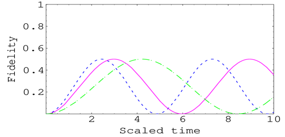
Figure 5: The same as Fig.$4$, with $C_{j}/C_{g}=5$ and $\Delta=0.1$ where the dot, the solid and the dash curves for $n=3,2,1$ respectively.

Let us assume that Alice measures $\bigl{|}\psi^{+}\bigr{\rangle}$, then the density operator on Bob’s hand is given by

$$\rho_{Bob}=\frac{1}{2}(|\lambda_{1}|^{2}|B_{n}|^{2}\bigl{|}0\bigr{\rangle}\bigl{\langle}0\bigr{|}+\lambda_{1}\lambda_{2}^{*}B_{n}A_{n}^{*}\bigl{|}0\bigr{\rangle}\bigl{\langle}1\bigr{|}+\lambda_{2}^{*}\lambda_{1}A_{n}B_{n}^{*}+|\lambda_{2}|^{2}|A_{n}|^{2}\bigl{|}1\bigr{\rangle}\bigl{\langle}1\bigr{|}),$$ (11)

with,

$$A_{n}=\cos(\gamma\mu_{n}\tau)-\frac{i\Delta}{\mu_{n}}\sin(\gamma\mu_{n}\tau),\quad B_{n}=\frac{i\lambda\sqrt{n}}{\mu_{n}}\sin(\mu_{n}t)$$ (12)

where, we assume that the Cooper pair box is prepared on the ground state and the field on the Fock state i.e $\bigl{|}\psi_{0}\bigr{\rangle}=\bigl{|}g,n\bigr{\rangle}$. In Fig.4, we plot the of the fidelity of the teleported state (11), for different values of the field and the Cooper pair parameters. The effect of the detuning parameter is seen in Fig.(4a), where we assume that there is only one photon inside the cavity and the ratio $C_{jg}=5$. From this figure it is clear that as one increases $\Delta$, the fidelity of the teleported state decreases. This due to that for large values of the detuning parameter, the degree of entanglement decreases as it is clear from Fig.$(1f)$. Since, the entangled time, the time in which the entanglement survival, increases for small values of the detunang parameter, the fidelity vanishes for large values of $\Delta$ much faster. The effect of $C_{jg}$ is shown in Fig.(4b),where for small values of this ratio, the fidelity reaches to its maximum value faster than the large values of $C_{jg}$. On the other hand the different values of this ratio has no effect on the maximum values of the fidelity. Also, as one increases this ratio, the interval of time in which the channel is available for quantum teleportation increases.

In Fig.(5), we investigate the effect of different values of the number of photons inside the cavity, where we fixed the other parameters. It is clear that for small values of $n$, the possibility of sending information with non-vanishing fidelity by using the quantum teleportation increases. This is due to that for large values of $n$, the possibility of quick interaction increases and consequently one can gets an entangled state much faster.

5 Conclusion

We employ the Cooper pair box to generate entangled state by interacting with a single cavity mode is initially prepared in the numbers state. We show that it is possible to generate a maximum entangled state by controlling on the capacities and the detuning parameters. Also, one can use the generated entangled state to perform the quantum teleportation. We investigate the effect of the detuning parameter, the ratio of capacities and the photon inside the cavity on the fidelity of the teleported state. For small values of the detuning parameter and the photon numbers inside the cavity one can teleportate the given state with large fidelity. On the other hand by increasing the ratio of the capacities one can enlarge the interval of time in which one can teleportate the state with non-vanishing fidelity.

References

- [1] D. V. Averin, Solid State Communications, 105 659 (1998); Y. Makhlin, G.Schon, and A. Shnirman, Nature 398 305 (1999).
- [2] J. Mooij, T. Orlando, L. Levitov, L. Tian, C. H. van der Wal, and S. Lloyd, Science 285 1036 (1999).
- [3] A. Blais, A. Zagoskin Phy. Rev. A, 61, 042308 (2000).
- [4] D. Loss, D. DiVincenzo, Phys. Rev. A 57, 120 (1998).
- [5] M. Zhang, J. Zpu and B. Shao, Int. J. Mod. Phys. B16 4767 (2002), W. Krech and T. Wanger, Phys. Lett A 275 159 (2000), H. S. Ding, S. P. Zhao, G. H. Chen and Q. S. Yang, Physica C382 431 (2002).
- [6] Yu. Makhlin, G. Schön and A. Shnirman, Nature 398 305 (1999); G. Schön, Yu. Makhlin and A. Shnirman, Physica C352 113(2001); J. Q. You and F. Nori, Physica E 18 33 (2003).
- [7] G. Wendin, R. Soc. Lond. A 361 1323 (2003), A. Niskanen, J. Vartiainen, and M. Salomaa, Phys. Rev. Lett.90 197901 (2003).
- [8] C. H. Bennett, G. Brassard, C. Crepeau, R. Jozsa, A. Peres, and W. Wootters, Phys. Rev. Lett. 70, 1895 (1993).
- [9] A. Cabello, Phys. Rev. Lett 89, 100402 (2003); B. Zeng, X. S. Liu, S. Y. Li and G. L. Long, Commun. Theor Phys. 38 537 (2003).
- [10] H,-J. Cao, H. C. Zhong and S. He-Shan, Phys. Scr 78 015002 (2008).
- [11] D. Bouwmeester, J.-W. Pan, K.Mattle,M. Eible, H.Weinfurter, and A. Zeilinger, Nature 390, 575 (1997); D. Boschi, S. Branca, F. D. Martini, L. Hardy, and S. Popescu, Phys. Rev. Lett.80 1121 (1998).
- [12] R. Migliore, A. Messina, A. Napoli, Eur. Phys. J. B 13 585 (2000);R. Migliore, A. Messina, A. Napoli, Eur. Phys. J. B 22 111 (2001).
- [13] Y. Makhlin, G. Schon and A. Shnirman, Rev. Mod. Phys. 73 357 (2001).
- [14] T. S. Tsai, Y. Nakamura and Yu. Pashkin, Physica C 367191 (2002); Yu. A. Pashkin, T, Yamamoto, O. Astafiev, Y. Nakamura, D, Averin, T. Tilma, F. Nori and J. S. Tsai, Physica C 4261552 (2005).
- [15] J. You, F.Nori, Physica E18 33 (2003).
- [16] A. Peres, Phys. Rev. Lett. A 77, 1413 (1996).
- [17] M. Horodecki, P. Horodecki, R. Horodecki, Phys. Lett.A 222 1 (1996).
- [18] S. Hill, W. K. Wootters, Phys. Rev. Lett.,78 5022 (1997).
- [19] C. H. Bennett, H. J. Bernstein, S. Popescu, B. Schummacher, Phys. Rev. A 532046 (1996).
- [20] W. K. Wootters, Phys. Rev. Lett.80 2245 (1998).
- [21] P. Horodecki, Phys. Lett A232 333(1997); J. Eisert, M. B. Plenio, J, Mod. Opt. 46145 (1999); J. Lee, M. S. Kim, Y. J. Park, S. Lee, J. Mod. Opt. 47 2151 (2000).
- [22] T. Yu and J. H. Eberly, Opt. Commu.264 393 (2006); M. Yonac, T. Yu and J. H. Eberly, J. Phys. B39 S621 (2006); T Yu and J. H. Eberly; J. Mod. Opt. 54, 2289-2296 (2007).
- [23] Z. Ficek and R. Tanas, quant/ph :08024287 (2008); M. Abdel-Aty and T. Yu, quant/ph 0805.3576 (2008).