Demonstration of a quantum nondemolition sum gate

Abstract

The sum gate is the canonical two-mode gate for universal quantum computation based on continuous quantum variables. It represents the natural analogue to a qubit C-NOT gate. In addition, the continuous-variable gate describes a quantum nondemolition (QND) interaction between the quadrature components of two light fields. We experimentally demonstrate a QND sum gate, employing the scheme by R. Filip, P. Marek, and U.L. Andersen [Phys. Rev. A71, 042308 (2005)], solely based on offline squeezed states, homodyne measurements, and feedforward. The results are verified by simultaneously satisfying the criteria for QND measurements in both conjugate quadratures.

The analogue of a two-qubit C-NOT gate, when continuous quantum variables are considered, is the so-called sum gate. It represents the canonical version of a two-mode entangling gate for universal quantum computation in the regime of continuous variables Bartlett . When applied to two optical, bosonic modes, as opposed to a simple beam splitter transformation, the sum gate is even capable of entangling two modes each initially in a coherent state, i.e., a close-to-classical state.

Apart from representing a universal two-mode gate, the sum gate also describes a quantum nondemolition (QND) interaction. The concept of a QND measurement has been known for almost 30 years. Initially, it was proposed to allow for better accuracies in the detection of gravitational waves QND . A QND measurement is a projection measurement onto the basis of a QND observable which is basically a constant of motion. The QND measurement should preserve the measured observable, but still gain sufficient information about its value; the back action is confined to the conjugate observable.

Various demonstrations of QND or backaction evading measurements have been reported QND_experiment . The interest in the realization of a full QND gate grew only recently, mainly in the context of continuous-variable (CV) quantum information processing SamPvLRMP . In particular, the QND sum gate is (up to local phase rotations) the canonical entangling gate for building up Gaussian cluster states clusterZhang , a sufficient resource for universal quantum computation clusterMenicucci . Other applications of the sum gate are CV quantum error correction QEC and CV coherent communication coherent_communication .

Here we report on the experimental demonstration of a full QND sum gate. The gate leads to quantum correlations in both conjugate variables, consistent with an entangled state, and allowing for a QND measurement of either variable with signal and probe interchanged. While previous works focused on fulfilling the criteria for a QND measurement QND_criteria of one fixed variable, here we satisfy the QND criteria for two non-commuting observables, verifying entanglement at the same time. As our implementation is very efficient and controllable, the current scheme can be used to process arbitrary optical quantum states, including fragile non-Gaussian states. Similar to the measurement-based implementation of single-mode squeezing gates Filip05.pra ; Yoshikawa07.pra , realization of the QND gate only requires two offline squeezed ancilla modes Filip05.pra ; Braunstein05.pra .

Let us write the QND-gate Hamiltonian as $\hat{H}_{\text{QND}}=\hat{x}_{1}\hat{p}_{2}$, with a suitable choice of the absolute phase for each mode. Here $\hat{x}/2$ and $\hat{p}/2$ are the real and imaginary parts of each mode’s annihilation operator, $\hat{a}=(\hat{x}+i\hat{p})/2$, and the subscripts ‘1’ and ‘2’ denote two independent modes. The ideal QND input-output relations then become,

$$\hat{x}_{1}^{\text{out}}= \hat{x}_{1}^{\text{in}}, \hat{x}_{2}^{\text{out}}= \hat{x}_{2}^{\text{in}}+G\hat{x}_{1}^{\text{in}},$$

$$\hat{p}_{1}^{\text{out}}= \hat{p}_{1}^{\text{in}}-G\hat{p}_{2}^{\text{in}}, \hat{p}_{2}^{\text{out}}= \hat{p}_{2}^{\text{in}},$$ (1)

where $G$ is the gain of the interaction.

Through this ideal QND interaction, the “signal” QND variable $\hat{x}_{1}$ ($\hat{p}_{2}$) is preserved in the output state and its value is added to the “probe” variable $\hat{x}_{2}$ ($\hat{p}_{1}$). This allows for a QND measurement of either $\hat{x}_{1}$ or $\hat{p}_{2}$, with a back action confined to the conjugate variable. The usual criteria for QND measurements (in the linearized, Gaussian regime) are QND_criteria ,

$$1<T_{\text{S}}+T_{\text{P}} \leq 2, V_{\text{S}|\text{P}} <1,$$ (2)

where $T_{\text{S}}$ and $T_{\text{P}}$ are the transfer coefficients from signal input to signal output (“signal preservation”) and from signal input to probe output (“information gain”), respectively; $V_{\text{S}|\text{P}}$ is the conditional variance of the signal output when the probe output is measured (“quantum state preparation”).

The implementation of the QND gate based on offline resources is shown in Fig. 1. The interaction gain $G$ in Eq. (1) is related to the reflectivities of the four beam splitters via one free parameter $R$, with $G=\left(1/\sqrt{R}\right)-\sqrt{R}$, taking arbitrary values for $0<R\leq 1$. The full scheme is described by the input-output relations Filip05.pra ,

$$\hat{x}_{1}^{\text{out}}= \hat{x}_{1}^{\text{in}}-\sqrt{\frac{1-R}{1+R}}\,\hat{x}_{\text{A}}^{(0)}e^{-r_{\text{A}}},$$ (3)

$$\hat{x}_{2}^{\text{out}}= \hat{x}_{2}^{\text{in}}+\frac{1-R}{\sqrt{R}}\hat{x}_{1}^{\text{in}}+\sqrt{R\,\frac{1-R}{1+R}}\,\hat{x}_{\text{A}}^{(0)}e^{-r_{\text{A}}},$$ (4)

$$\hat{p}_{1}^{\text{out}}= \hat{p}_{1}^{\text{in}}-\frac{1-R}{\sqrt{R}}\hat{p}_{2}^{\text{in}}+\sqrt{R\,\frac{1-R}{1+R}}\,\hat{p}_{\text{B}}^{(0)}e^{-r_{\text{B}}},$$ (5)

$$\hat{p}_{2}^{\text{out}}= \hat{p}_{2}^{\text{in}}+\sqrt{\frac{1-R}{1+R}}\,\hat{p}_{\text{B}}^{(0)}e^{-r_{\text{B}}},$$ (6)

where $\hat{x}_{\text{A}}^{(0)}e^{-r_{\text{A}}}$ and $\hat{p}_{\text{B}}^{(0)}e^{-r_{\text{B}}}$ are the squeezed quadratures of the ancilla modes, leading to some excess noise for finite squeezing. The gate operation becomes ideal in the limit of infinite squeezing ($r_{\text{A}},r_{\text{B}}\rightarrow\infty$). Note that here precise control of active squeezing arising from an unstable process of parametric down conversion is not needed; instead, the gate is completely controlled via passive optical devices. For sufficiently large squeezing of the ancilla modes, this transformation also allows for QND measurements. Using variable beam splitters, we experimentally realized two interaction gains, $G=1.0$ and $1.5$. In particular, the unit gain interaction is significant for quantum information processing. Nonetheless, we observe a better performance in the QND measurements using higher gain. We note that a non-unitary and single quadrature QND measurement based on squeezed vacuum and feedforward has been demonstrated in Ref. Buchler02 .

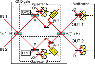
Figure 1: (Colors online) Schematic of the experimental setup. The parameter $R$ determines the reflectivities of the four beam splitters, which are $1/(1+R),$ $R,$ $R,$ and $R/(1+R)$. We employ optical parametric oscillators (OPO) to produce ancilla squeezed vacuum modes, local oscillators (LO) for homodyne detection, and electro-optic modulators (EOM) combined with highly asymmetric beam splitters (99:1) for signal displacement.

Experimental setup. A schematic of the experimental setup is illustrated in Fig. 1. It basically consists of a Mach-Zehnder interferometer with a single-mode squeezing gate in each arm. To implement fine-tunable and lossless squeezing operations, we use the measurement-induced squeezing approach proposed in Ref. Filip05.pra , experimentally implemented in Ref. Yoshikawa07.pra and illustrated inside the dashed boxes of Fig. 1.

We define the modes of the system to be residing at frequency sidebands of $1.25$ MHz relative to the optical carrier of the bright continuous wave light beam at a wavelenght of 860 nm from a Ti:sapphire laser. The powers in each of the two input modes and the squeezed modes are 10 $\mu$W and 2 $\mu$W, respectively. These powers are considerably smaller than the powers (3 mW) of the local oscillators (LOs) used for homodyne detection. All the interferences at the beam splitters are actively phase locked using modulation sidebands of 77 kHz, 106 kHz, and their beat in 29 kHz. Subthreshold optical parametric oscillators (OPOs) generate the squeezed vacuum ancillas. To control the beam splitting ratios of the four beam splitters in the squeezing operations and the Mach-Zehnder interferometer, they are composed of two polarizing beam splitters and a half wave plate Yoshikawa07.pra .

The OPOs are bow-tie shaped cavities of 500 mm in length, containing a periodically-poled KTiOPO₄ (PPKTP) crystal of 10 mm in length. The pump beams for the OPOs (with wavelengths of 430 nm and powers of about 100 mW) are the second harmonic of the output of the Ti:sapphire laser. The frequency doubling cavity (not shown in the figure) has the same configuration as the OPOs, but contains a KNbO₃ crystal. For details of a squeezed vacuum generation, see Ref. Suzuki06.apl . Each OPO enables a squeezing degree of about $-5$ dB relative to the shot noise limit.

The outcomes of the homodyne detections in the QND gate are fed forward to the remaining part. After low noise electric amplification, they drive an electro-optical modulator (EOM) traversed by an auxiliary beam with the power of 150 $\mu$W, which is subsequently mixed with the signal beam by a highly asymmetric beam splitter (99:1).

The QND scheme is characterized by measuring the two input modes as well as the two output modes using homodyne detection. The detector’s quantum efficiencies are higher than 99%, the interference visibilities to the LOs are on average 98%, and the dark noise of each homodyne detector is about 17 dB below the optical shot noise level produced by the local oscillator. We measure the propagation losses in each of the two main modes through the QND apparatus to be about 7%.

Experimental results. The three measures in Eq. (2) are used to quantify the performance of our QND system. To estimate them, we perform measurements of the second moments of the input fields and the output fields, employing a spectrum analyzer with a center frequency of 1.25 MHz, resolution and video bandwidths of 30 kHz and 300 Hz, respectively, a sweep time set to $0.1$ s and further averaging of 20 traces. In Fig. 2-4 the results for $G=1.0$ are shown as an example; in Table 1 the performance of the QND device is listed for both $G=1.0$ and $G=1.5$.

In the first series of measurements we determine the variances of conjugate quadratures of the output states when the input states are pure vacua. The results corresponding to $G=1.0$ are presented in Fig. 2. The variances of the two input states are at the vacuum noise level as illustrated by the blue traces. As a result of the QND interaction, in the ideal case, the noise of the signal variables ($\hat{x}_{1}$ and $\hat{p}_{2}$) is added to the probe variables ($\hat{x}_{2}$ and $\hat{p}_{1}$), while the signal variables are preserved. The expected variances for the ideal performance is marked by the yellow lines and the actual measured variances of the output state is given by the red traces. The deviation from the ideal performance is due to the finite amount of squeezing for the ancillas. For comparison, we also measure the variances of the output states when no squeezing is used. This is shown by the green traces. The expected variances, for finite squeezing or without squeezing, are calculated and marked by pink and light green lines, respectively.

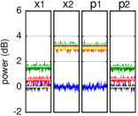
Figure 2: (Colors) Power spectra for input and output states corresponding to vacuum inputs and the interaction gain of $G=1.0$. Shown are the experimental QND output variances (red) with their theoretically calculated values (pink) compared to the results with vacuum-state ancillas (green) and their theoretical values (light green). The yellow lines refer to the theoretical results for infinite squeezing and the blue traces show the shot noise level corresponding to the variances of the input states.

In the second series of measurements, in order to test the universality of the QND gate, we replace the input vacuum states by a pair of coherent states. We generate the coherent amplitude in each quadrature of the two input modes by modulating the amplitude or phase of their carriers using an EOM operating at $1.25$ MHz. We investigate four different input states, each corresponding to a coherent excitation in, respectively, (a) $x_{1}^{\text{in}}$, (b) $x_{2}^{\text{in}}$, (c) $p_{1}^{\text{in}}$ and (d) $p_{2}^{\text{in}}$. The measurement results of the second moments of the input and output modes for $G=1.0$ are shown in Fig. 3. The excitations of the input modes are measured by setting the reflectivities of the four beam splitters to unity and blocking the auxiliary displacement beams in the feedforward construction. These measurements are illustrated by the blue traces (the non-excited quadratures are not shown because they are at the vacuum level, 0 dB). Traces in red are the second moments of the output modes. We observe that the amplitude of the input states is preserved in the same quadrature with almost unity gain. Furthermore, we clearly see the expected feature that the information in a signal variable, $\hat{x}_{1}^{\text{in}}$ or $\hat{p}_{2}^{\text{in}}$, is coupled into the probe variable $\hat{x}_{2}^{\text{out}}$ or $\hat{p}_{1}^{\text{out}}$ (see Fig. 3(a) and (d)), whereas the amplitude in the probe variables $\hat{x}_{2}^{\text{in}}$ and $\hat{p}_{1}^{\text{in}}$ does not couple to any of the other quadratures (see Fig. 3(b) and (c)). These results verify the interaction in Eq. (1). From these measurements we determine the transfer coefficients $T_{\text{S}}$ and $T_{\text{P}}$ using the method outlined in ref. poizat94 . The results are summarised in table 1.

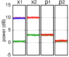
(a) Amplitude in $x_{1}^{\text{in}}$.

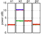
(b) Amplitude in $x_{2}^{\text{in}}$.

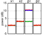
(c) Amplitude in $p_{1}^{\text{in}}$.

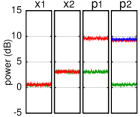
(d) Amplitude in $p_{2}^{\text{in}}$.

Figure 3: (Colors) Power spectra for the input and output states corresponding to four different input states for $G=1.0$. The excited input quadratures are shown in blue (non-excited input quadratures with variances equal to the shot noise level are not shown). The power spectra of the output quadratures are in red, and, for comparison, we added the spectra corresponding to the measurements without squeezed ancilla states.

Finally, we measure the conditional variance using the setup shown in Fig. 4(a). The outcomes from one of the homodyne detectors are rescaled by a gain $g$, subtracted from (or added to) the outcomes of the other homodyne detector and subsequently directed to a spectrum analyzer. The resulting normalized noise powers are shown in Fig. 4(b) and (c) as a function of the rescaling gain $g$. The minima of these plots correspond to the conditional variances for the various realizations: curve (i) represents ideal performance, curve (ii) is associated with our system with finitely squeezed ancillas, and curve (iii) is the performance of the system without squeezed ancilla states. The parabolic curves are theoretical calculations, and the dots with vertical error bars along the curves (ii) and (iii) are the experimental results. The conditional variances, $V_{\text{S}|\text{P}}$, are collected in table 1.

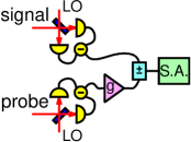
(a) Setup of verification part.

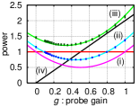
(b) Variances of ($\hat{x}_{1}^{\text{out}}-g\hat{x}_{2}^{\text{out}}$).

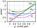
(c) Variances of ($\hat{p}_{2}^{\text{out}}+g\hat{p}_{1}^{\text{out}}$).

Figure 4: (Colors online) Differential quadrature power spectra of the two output states resulting in measurements of the conditional variances. (a) Experimental setup for determining the conditional variance. The measured probe quadrature is rescaled with a variable gain $g$, added (subtracted) ($\pm$) to (from) the signal mode detector output, and analyzed with an electronic spectrum analyzer (S.A.). Variances of $\hat{x}_{1}^{\text{out}}-g\hat{x}_{2}^{\text{out}}$ and of $\hat{p}_{2}^{\text{out}}+g\hat{p}_{1}^{\text{out}}$ are shown in (b) and (c), respectively: theoretical prediction for an ideal QND interaction (i), a QND interaction with a finite degree of squeezing of the ancilla modes (ii), and with vacuum ancilla modes (iii). By entering the areas below the lines (iv) entanglement is verified. The vertical axes are variances normalized to the shot noise power of the signal variable.

G	1.0		1.5
Quadrature	$x$	$p$	$x$	$p$
$T_{\text{S}}$	$0.79\pm 0.03$	$0.71\pm 0.03$	$0.80\pm 0.03$	$0.71\pm 0.03$
$T_{\text{P}}$	$0.41\pm 0.02$	$0.39\pm 0.02$	$0.62\pm 0.03$	$0.56\pm 0.02$
$T_{\text{S}}+T_{\text{P}}$	$1.20\pm 0.05$	$1.10\pm 0.05$	$1.42\pm 0.06$	$1.27\pm 0.05$
$V_{\text{S}|\text{P}}$	$0.75\pm 0.01$	$0.78\pm 0.01$	$0.61\pm 0.01$	$0.63\pm 0.01$

Table 1: Evaluation of the QND interaction. Shown are the quadrature transfer coefficients $T_{\text{S}}$ and $T_{\text{P}}$ and the conditional variance $V_{\text{S}|\text{P}}$ for two different gains G.

Our experiment demonstrates the realization of a canonical two-mode entangling gate. From the output-output correlations in Fig. 4, we verify entanglement between the two output modes. According to Duan and Simon Duan00 ; Simon00 , a sufficient condition for an entangled state is,

$$\langle{(\hat{x}_{1}^{\text{out}}-g\hat{x}_{2}^{\text{out}})^{2}}\rangle+\langle{(\hat{p}_{2}^{\text{out}}+g\hat{p}_{1}^{\text{out}})^{2}}\rangle<4|g|,$$ (7)

where $g$ is the rescaling gain. Thus, if the parabolic curves in Fig. 4 (b) and (c) go below the lines (iv) simultaneously for both quadratures, the two output modes are entangled, which is the case for curves (ii) with squeezed ancillas. Note that the two-mode gate here has been applied to two coherent input states which, without the squeezed ancillas, would not become entangled via any linear optical transformation alone (see, e.g., curve (iii)).

In conclusion, we have demonstrated and fully characterized a close-to-unitary quantum nondemolition sum gate using only linear optics and offline squeezed vacuum states. The performance of the sum gate was quantified by applying the usual QND criteria to each conjugate quadrature; we found that the gate operates in the quantum regime, entangling even two input coherent states. The future prospects of this demonstration are intriguing since the sum gate is an integral part of e.g. a one-way quantum computer based on continuous variables clusterMenicucci and quantum error correction protocols QEC .

This work was partly supported by SCF and GIA commissioned by the MEXT of Japan, and the Research Foundation for Opt-Science and Technology. ULA and AH acknowledge financial support from the EU under project No. 212008 (COMPAS) and the Lundbeck foundation. PvL acknowledges support from the Emmy Noether programme of the DFG in Germany.

References

- (1) S.D. Bartlett et al., Phys. Rev. Lett. 88, 097904 (2002).
- (2) C.M. Caves et al., Rev. Mod. Phys. 52 341 (1980).
- (3) For example, Z.Y. Pereira et al., Phys. Rev. Lett. 72, 214 (1994).
- (4) S.L. Braunstein and P. van Loock, Rev. Mod. Phys. 77, 513 (2005).
- (5) J. Zhang and S.L. Braunstein, Phys. Rev. A73, 032318 (2006).
- (6) N.C. Menicucci et al., Phys. Rev. Lett. 97, 110501 (2006).
- (7) S.L. Braunstein, Phys. Rev. Lett. 80, 4084 (1998); S. Lloyd and J.-J.E. Slotine, Phys. Rev. Lett. 80, 4088 (1998).
- (8) M.M. Wilde et al., Phys. Rev. A75, 060303(R) (2007).
- (9) M.J. Holland et al., Phys. Rev. A42 2995 (1990).
- (10) R. Filip et al., R. Filip, P. Marek, and U.L. Andersen, Phys. Rev. A 71, 042308 (2005).
- (11) J. Yoshikawa et al., Phys. Rev. A76, 060301(R) (2007).
- (12) S.L. Braunstein, Phys. Rev. A71, 055801 (2005).
- (13) B.C. Buchler et al., Phys. Rev. A65, 011803(R) (2002).
- (14) S. Suzuki et al., Appl. Phys. Lett. 89, 061116 (2006).
- (15) J.-Ph. Poizat et al., Ann. Phys. (Paris) 19, 265 (1994).
- (16) L.-M. Duan et al., Phys. Rev. Lett. 84, 2722 (2000).
- (17) R. Simon, Phys. Rev. Lett. 84, 2726 (2000).