Evolution to a smooth universe in an ekpyrotic contracting phase with $w>1$

Abstract

A period of slow contraction with equation of state $w>1$, known as an ekpyrotic phase, has been shown to flatten and smooth the universe if it begins the phase with small perturbations. In this paper, we explore how robust and powerful the ekpyrotic smoothing mechanism is by beginning with highly inhomogeneous and anisotropic initial conditions and numerically solving for the subsequent evolution of the universe. Our studies, based on a universe with gravity plus a scalar field with a negative exponential potential, show that some regions become homogeneous and isotropic while others exhibit inhomogeneous and anisotropic behavior in which the scalar field behaves like a fluid with $w=1$. We find that the ekpyrotic smoothing mechanism is robust in the sense that the ratio of the proper volume of the smooth to non-smooth region grows exponentially fast along time slices of constant mean curvature.

I Introduction

For over two decades, the only known mechanism for homogenizing, isotropizing and flattening the universe was inflation, a period of accelerated expansion with an equation of state $w$ (ratio of pressure to energy density) near -1. Its success in resolving the horizon and flatness problems is a principal reason why inflation became an essential part of the standard model of cosmology. In recent years, an alternative mechanism has been discovered in which smoothing and flattening occurs before the big bang as the universe undergoes a period of slow contraction with $w>1$. This alternative, known as the ekpyrotic mechanism Khoury:2001wf ; Erickson:2003zm , has been incorporated in alternatives to standard big bang inflationary cosmology including the “ekpyrotic” Khoury:2001wf , “new ekpyrotic” Buchbinder:2007ad and cyclic models Steinhardt:2002ih . We note that both the inflationary and ekpyrotic mechanisms can produce nearly scale-invariant spectra for density perturbations in addition to smoothing and flattening the universe.

Until now, the ekpyrotic mechanism has only been shown to work in cases where the deviations from smoothness and flatness are small and perturbative when the ekpyrotic phase begins. The purpose of this paper is to show that the ekpyrotic mechanism is powerful and robust enough to smooth the universe even when the initial perturbations are large and non-linear.

Let us first review how the inflation and the ekpyrotic mechanism work in the perturbative regime where the cosmic evolution is well approximated by the Friedmann equation with an anisotropy term:

$$H^{2}=\frac{8\pi G}{3}\left(\frac{\rho_{m}^{0}}{a^{3}}+\frac{\rho_{r}^{0}}{a^{4}}+\frac{\rho_{w}^{0}}{a^{3(1+w)}}\right)-\frac{k}{a^{2}}+\frac{\sigma^{2}}{a^{6}},$$ (1)

where $H\equiv\dot{a}/{a}$ is the Hubble parameter; $a(t)$ is the Friedmann-Robertson-Walker scale factor normalized so that the value today, $t_{0}$, is $a(t_{0})=1$; $\rho_{i}^{0}$ represents the present value of the energy density for component $i$, where $m$ represents non-relativistic matter, $r$ represents radiation and $w$ represents an energy component with equation of state $w$, such as a scalar field and its potential. The last two terms on the right-hand side represent spatial curvature and anisotropy.

For an expanding universe, the term that dominates Eq. (1) after a long period of expansion is the one with the smallest power of $a$ in the denominator. With only radiation and matter, the dominant term would be the spatial curvature, leading to a universe that is unacceptably open or closed by the present epoch. However, introducing an energy component with $w\approx-1$ totally changes the outcome because this component ($\rho_{w}$) then has the smallest exponent and dominates the Einstein equation, while the curvature and anisotropy (and other energy components) become negligible. This is the essence of how inflation works if the initial conditions are perturbative. For inflation, there are several “Cosmic No-hair” theorems in addition to numerical results supporting the claim that homogeneity, isotropy and flatness develop even when the initial conditions are non-linear and non-perturbative kolb_turner_86 ; Goldwirth .

Now consider the analogous arguments for a contracting universe. With $a(t)$ shrinking, the dominant term in Eq. (1) will be the one with the largest exponent of $a$ in the denominator. For a universe with matter and radiation only, this would be the anisotropy term, which famously overtakes the evolution and drives the universe into chaotic mixmaster behavior. On the other hand, if there is an energy component with $w>+1$, then this energy component dominates instead of anisotropy or spatial curvature, and chaotic mixmaster behavior never begins Erickson:2003zm . For a scalar field $\phi$ with potential energy density $V(\phi)$, the ratio of pressure to energy density is

$$w\equiv\frac{\frac{1}{2}\dot{\phi}^{2}-V}{\frac{1}{2}\dot{\phi}^{2}+V},$$ (2)

which can be significantly greater than unity when $V$ is less than zero and non-negligible and which approaches $w=1$ if the scalar field kinetic energy dominates. The ekpyrotic phase in ekpyrotic and cyclic models includes an effective scalar field component of this type.

For the cyclic model, the ekpyrotic phase is preceded by a period of dark energy domination and accelerated expansion which, if sustained long enough, would make the universe uniform and flat before the ekpyrotic contraction phase begins. In this case, the perturbative argument above should be reliable and sufficient to conclude that the universe is smooth and flat as it approaches the big crunch. However, in the ekpyrotic or new ekpyrotic models, generally, or in the cyclic model with a very short dark energy phase, the conditions at the beginning of the ekpyrotic phase are under less control.

This paper investigates the robustness of the ekpyrotic smoothing and flattening mechanism when the initial conditions are non-linear and non- perturbative to determine how the situation compares with the perturbative case and with inflation. For this study we are not concerned with any particular form for the initial conditions that may be motivated by some specific model; rather, we would like to understand how a generic, highly inhomogeneous and anisotropic space-time evolves under the influence of the proposed smoothing mechanism, modeled here by a scalar field with a negative exponential potential. Such negative exponential potentials arise naturally in supergravity and in string theory. Investigation of the proposed smoothing mechanism requires numerical solution of the coupled Einstein-scalar system of equations. For simplicity, we restrict our studies to deviations from smoothness along a single spatial dimension.

We use an orthonormal frame representation of the equations written in terms of Hubble-normalized, scale invariant variables Uggla:2003fp similar to that described in Curtis:2005va , though here coupling to a scalar field instead of a fluid, and using constant-mean-curvature (CMC) time slices. We discretize the equations using second-order accurate finite difference techniques, and solve them with a variant of the Berger and Oliger BO adaptive mesh refinement (AMR) algorithm for coupled elliptic-hyperbolic equations Pretorius:2005ua . We find smooth regions that are scalar field dominated in which the scalar field (kinetic plus potential energy density) component behaves like a fluid with $w\gg 1$, and also regions where the scalar field kinetic energy dominates over the potential energy and the scalar field behaves like a fluid with $w=1$. These latter regions remain inhomogeneous and anisotropic, and throughout this paper we will refer to these parts of the universe as the “anisotropic regions”. Note however that the anisotropic regions are neither anisotropy nor matter dominated because both the scalar field and the anisotropy of the metric play important roles in the dynamics. Futhermore, note that despite the fact that matter in the smooth regions behaves effectively like a fluid with $w\gg 1$ there is no issue of superluminal propagation as might arise from an actual fluid with such an equation of state. This is because we are always solving the scalar wave equation with potential where disturbances always propagate within the light cone. In the anisotropic regions “spikes” also form, which are places where the fields change on very small spatial scales, and are similar to regions with this property that have been observerd in numerical simulations of singularities in vacuum spacetimesdgspike . Despite the presence of the scalar field, the anisotropic regions exhibit dynamical behavior similar to chaotic mixmaster vacuum solutions, where there are a series of relatively quick transitions between longer epochs where the solution can be described by a $w=1$ Bianchi type I spacetime. A difference here though is that there are only a finite number of transistions, so the mixmaster behavior terminates after several transitions. These dynamics are also known to occur in spacetimes where the matter is a fluid with $w=1$ Curtis:2005va ; Coley05 . AMR is necessary to resolve the spiky features that form both in the anisotropic regions and, in some instances, briefly in what will eventually become smooth scalar field dominated regions, and to resolve the almost domain wall-like transitions that develop between the smooth and anisotropic regions.

The outline for the rest of the paper is as follows. In Sec. II we describe the equations, initial conditions, and numerical methods used to solve them. We present the results in Sec. III. The primary conclusion is that a scalar field with a potential inspired by cyclic models is a remarkably powerful and robust smoothing mechanism during a contracting phase of the universe, able to drive the spacetime to homogeneity and isostropy even starting with highly non-linear deviations from an FRW spacetime. Concluding remarks and a discussion of future work is given in Sec. IV.

II the equations and solution method

The method we use to evolve the Einstein-scalar equations is the scale invariant tetrad method of Uggla et al. Uggla:2003fp . We use this method with constant mean curvature slicing as is done in the vacuum simulations of dgaei but with scalar field matter instead of vacuum. Thus our system can be thought of as the system of dgaei but with extra variables and equations describing the matter, and with extra source terms for the influence of the matter on the metric evolution equations. More information on this type of method can be found in Uggla:2003fp ; dgaei .

The spacetime is described in terms of a coordinate system ($t,{x^{i}}$) and a tetrad (${{\bf e}_{0}},{{\bf e}_{\alpha}}$) where both the spatial coordinate index $i$ and the spatial tetrad index $\alpha$ go from 1 to 3. Choose ${\bf e}_{0}$ to be hypersurface orthogonal with the relation between tetrad and coordinates of the form ${{\bf e}_{0}}={N^{-1}}{\partial_{t}}$, and ${{\bf e}_{\alpha}}={{e_{\alpha}}^{i}}{\partial_{i}},$ where $N$ is the lapse and the shift is chosen to be zero. Choose the spatial frame $\{{{\bf e}_{\alpha}}\}$ to be Fermi propagated along the integral curves of ${\bf e}_{0}$. The commutators of the tetrad components are decomposed as follows:

$$[{{\bf e}_{0}},{{\bf e}_{\alpha}}] = {{\dot{u}}_{\alpha}}{{\bf e}_{0}}-(H{{\delta_{\alpha}}^{\beta}}+{{\sigma_{\alpha}}^{\beta}}){{\bf e}_{\beta}}$$ (3)

$$\left[{{\bf e}_{\alpha}},{{\bf e}_{\beta}}\right] = (2{a_{[\alpha}}{{\delta_{\beta]}}^{\gamma}}+{\epsilon_{\alpha\beta\delta}}{n^{\delta\gamma}}){{\bf e}_{\gamma}},$$ (4)

where $n^{\alpha\beta}$ is symmetric, and $\sigma^{\alpha\beta}$ is symmetric and trace free. The scale invariant tetrad variables are defined by ${\kern-0.24994pt\hbox{$\partial$}\kern-5.30904pt\kern 0.50003pt\hbox{$\partial$}\kern-5.30904pt\kern-0.24994pt\raise 0.43304pt\hbox{$\partial$}_{0}}\equiv{{\bf e}_{0}}/H$ and ${\kern-0.24994pt\hbox{$\partial$}\kern-5.30904pt\kern 0.50003pt\hbox{$\partial$}\kern-5.30904pt\kern-0.24994pt\raise 0.43304pt\hbox{$\partial$}_{\alpha}}\equiv{{\bf e}_{\alpha}}/H$ while scale invariant versions of the other gravitational variables are given by

$$\{{{E_{\alpha}}^{i}},{\Sigma_{\alpha\beta}},{A^{\alpha}},{N_{\alpha\beta}}\}\equiv\{{{e_{\alpha}}^{i}},{\sigma_{\alpha\beta}},{a^{\alpha}},{n_{\alpha\beta}}\}/H.$$ (5)

Note that the relation between the scale invariant tetrad variables and the coordinate derivatives is

$${\kern-0.24994pt\hbox{$\partial$}\kern-5.30904pt\kern 0.50003pt\hbox{$\partial$}\kern-5.30904pt\kern-0.24994pt\raise 0.43304pt\hbox{$\partial$}_{0}} = {{\cal N}^{-1}}{\partial_{t}}$$ (6)

$${\kern-0.24994pt\hbox{$\partial$}\kern-5.30904pt\kern 0.50003pt\hbox{$\partial$}\kern-5.30904pt\kern-0.24994pt\raise 0.43304pt\hbox{$\partial$}_{\alpha}} = {{E_{\alpha}}^{i}}{\partial_{i}},$$ (7)

where ${\cal N}=NH$ is the scale invariant lapse. The matter model is a scalar field $\phi$ with potential $V$ of the form

$$V(\phi)=-V_{0}e^{-k\phi},$$ (8)

where $V_{0}$ and $k$ are positive constants. The scale invariant matter variables are given by

$$W = {\kern-0.24994pt\hbox{$\partial$}\kern-5.30904pt\kern 0.50003pt\hbox{$\partial$}\kern-5.30904pt\kern-0.24994pt\raise 0.43304pt\hbox{$\partial$}_{0}}\phi$$ (9)

$${S_{\alpha}} = {\kern-0.24994pt\hbox{$\partial$}\kern-5.30904pt\kern 0.50003pt\hbox{$\partial$}\kern-5.30904pt\kern-0.24994pt\raise 0.43304pt\hbox{$\partial$}_{\alpha}}\phi$$ (10)

$${\bar{V}} = V/{H^{2}}.$$ (11)

The time coordinate $t$ is chosen so that

$${e^{-t}}=3H.$$ (12)

Here we have used the scale invariance of the physical system to make both $t$ and $H$ dimensionless quantities. Note that equation (12) means that the surfaces of constant time are constant mean curvature surfaces. Note also that the singularity is approached as $t\to-\infty$.

Due to equation (12) the scale invariant lapse satisfies an elliptic equation

$$- {\kern-0.24994pt\hbox{$\partial$}\kern-5.30904pt\kern 0.50003pt\hbox{$\partial$}\kern-5.30904pt\kern-0.24994pt\raise 0.43304pt\hbox{$\partial$}^{\alpha}}{\kern-0.24994pt\hbox{$\partial$}\kern-5.30904pt\kern 0.50003pt\hbox{$\partial$}\kern-5.30904pt\kern-0.24994pt\raise 0.43304pt\hbox{$\partial$}_{\alpha}}{\cal N}+2{A^{\alpha}}{\kern-0.24994pt\hbox{$\partial$}\kern-5.30904pt\kern 0.50003pt\hbox{$\partial$}\kern-5.30904pt\kern-0.24994pt\raise 0.43304pt\hbox{$\partial$}_{\alpha}}{\cal N}$$ (13)

$$+ {\cal N}(3+{\Sigma_{\alpha\beta}}{\Sigma^{\alpha\beta}}+{W^{2}}-{\bar{V}})=3.$$

The gravitational quantities ${{E_{\alpha}}^{i}},\,{A_{\alpha}},{N^{\alpha\beta}}$ and $\Sigma_{\alpha\beta}$ satisfy the following hyperbolic evolution equations

$${\partial_{t}}{{E_{\alpha}}^{i}} = {{E_{\alpha}}^{i}}-{\cal N}({{E_{\alpha}}^{i}}+{{\Sigma_{\alpha}}^{\beta}}{{E_{\beta}}^{i}})$$ (14)

$${\partial_{t}}{A_{\alpha}} = {A_{\alpha}}+{\textstyle{\frac{1}{2}}}{{\Sigma_{\alpha}}^{\beta}}{\kern-0.24994pt\hbox{$\partial$}\kern-5.30904pt\kern 0.50003pt\hbox{$\partial$}\kern-5.30904pt\kern-0.24994pt\raise 0.43304pt\hbox{$\partial$}_{\beta}}{\cal N}-{\kern-0.24994pt\hbox{$\partial$}\kern-5.30904pt\kern 0.50003pt\hbox{$\partial$}\kern-5.30904pt\kern-0.24994pt\raise 0.43304pt\hbox{$\partial$}_{\alpha}}{\cal N}$$ (15)

$$+ {\cal N}\left({\textstyle{\frac{1}{2}}}{\kern-0.24994pt\hbox{$\partial$}\kern-5.30904pt\kern 0.50003pt\hbox{$\partial$}\kern-5.30904pt\kern-0.24994pt\raise 0.43304pt\hbox{$\partial$}_{\beta}}{{\Sigma_{\alpha}}^{\beta}}-{A_{\alpha}}-{{\Sigma_{\alpha}}^{\beta}}{A_{\beta}}\right)$$

$${\partial_{t}}{N^{\alpha\beta}} = {N^{\alpha\beta}}-{\epsilon^{\gamma\delta(\alpha}}{{\Sigma_{\delta}}^{\beta)}}{\kern-0.24994pt\hbox{$\partial$}\kern-5.30904pt\kern 0.50003pt\hbox{$\partial$}\kern-5.30904pt\kern-0.24994pt\raise 0.43304pt\hbox{$\partial$}_{\gamma}}{\cal N}+{\cal N}\Bigl{(}-{N^{\alpha\beta}}$$ (16)

$$+ 2{{N^{(\alpha}}_{\gamma}}{\Sigma^{\beta)\gamma}}-{\epsilon^{\gamma\delta(\alpha}}{\kern-0.24994pt\hbox{$\partial$}\kern-5.30904pt\kern 0.50003pt\hbox{$\partial$}\kern-5.30904pt\kern-0.24994pt\raise 0.43304pt\hbox{$\partial$}_{\gamma}}{{\Sigma_{\delta}}^{\beta)}}\Bigr{)}$$

$${\partial_{t}}{\Sigma_{\alpha\beta}} = {\Sigma_{\alpha\beta}}+{\kern-0.24994pt\hbox{$\partial$}\kern-5.30904pt\kern 0.50003pt\hbox{$\partial$}\kern-5.30904pt\kern-0.24994pt\raise 0.43304pt\hbox{$\partial$}_{<\alpha}}{\kern-0.24994pt\hbox{$\partial$}\kern-5.30904pt\kern 0.50003pt\hbox{$\partial$}\kern-5.30904pt\kern-0.24994pt\raise 0.43304pt\hbox{$\partial$}_{\beta>}}{\cal N}+{A_{<\alpha}}{\kern-0.24994pt\hbox{$\partial$}\kern-5.30904pt\kern 0.50003pt\hbox{$\partial$}\kern-5.30904pt\kern-0.24994pt\raise 0.43304pt\hbox{$\partial$}_{\beta>}}{\cal N}$$ (17)

$$+ {\epsilon_{\gamma\delta(\alpha}}{{N_{\beta)}}^{\delta}}{\kern-0.24994pt\hbox{$\partial$}\kern-5.30904pt\kern 0.50003pt\hbox{$\partial$}\kern-5.30904pt\kern-0.24994pt\raise 0.43304pt\hbox{$\partial$}^{\gamma}}{\cal N}+{\cal N}\Bigl{[}-3{\Sigma_{\alpha\beta}}-{\kern-0.24994pt\hbox{$\partial$}\kern-5.30904pt\kern 0.50003pt\hbox{$\partial$}\kern-5.30904pt\kern-0.24994pt\raise 0.43304pt\hbox{$\partial$}_{<\alpha}}{A_{\beta>}}$$

$$- 2{{N_{<\alpha}}^{\gamma}}{N_{\beta>\gamma}}+{{N^{\gamma}}_{\gamma}}{N_{<\alpha\beta>}}$$

$$+ {\epsilon_{\gamma\delta(\alpha}}({\kern-0.24994pt\hbox{$\partial$}\kern-5.30904pt\kern 0.50003pt\hbox{$\partial$}\kern-5.30904pt\kern-0.24994pt\raise 0.43304pt\hbox{$\partial$}^{\gamma}}{{N_{\beta)}}^{\delta}}-2{A^{\gamma}}{{N_{\beta)}}^{\delta}})+{S_{<\alpha}}{S_{\beta>}}\Bigr{]}$$

Here parentheses around a pair of indices denote the symmetric part, while angle brackets denote the symmetric trace-free part.

The equations of motion for the matter variables are as follows:

$${\partial_{t}}\phi = {\cal N}W$$ (18)

$${\partial_{t}}{S_{\alpha}} = {S_{\alpha}}+W{\kern-0.24994pt\hbox{$\partial$}\kern-5.30904pt\kern 0.50003pt\hbox{$\partial$}\kern-5.30904pt\kern-0.24994pt\raise 0.43304pt\hbox{$\partial$}_{\alpha}}{\cal N}$$ (19)

$$+ {\cal N}\left[{\kern-0.24994pt\hbox{$\partial$}\kern-5.30904pt\kern 0.50003pt\hbox{$\partial$}\kern-5.30904pt\kern-0.24994pt\raise 0.43304pt\hbox{$\partial$}_{\alpha}}W-({S_{\alpha}}+{{\Sigma_{\alpha}}^{\beta}}{S_{\beta}})\right]$$

$${\partial_{t}}W = W+{S^{\alpha}}{\kern-0.24994pt\hbox{$\partial$}\kern-5.30904pt\kern 0.50003pt\hbox{$\partial$}\kern-5.30904pt\kern-0.24994pt\raise 0.43304pt\hbox{$\partial$}_{\alpha}}{\cal N}$$ (20)

$$+ {\cal N}\left({\kern-0.24994pt\hbox{$\partial$}\kern-5.30904pt\kern 0.50003pt\hbox{$\partial$}\kern-5.30904pt\kern-0.24994pt\raise 0.43304pt\hbox{$\partial$}^{\alpha}}{S_{\alpha}}-3W-2{A^{\alpha}}{S_{\alpha}}-{\frac{\partial{\bar{V}}}{\partial\phi}}\right).$$

In addition, the variables are subject to the vanishing of the following constraint quantities

$${{({{\cal C}_{\rm com}})}^{\lambda i}} = {\epsilon^{\alpha\beta\lambda}}[{\kern-0.24994pt\hbox{$\partial$}\kern-5.30904pt\kern 0.50003pt\hbox{$\partial$}\kern-5.30904pt\kern-0.24994pt\raise 0.43304pt\hbox{$\partial$}_{\alpha}}{{E_{\beta}}^{i}}-{A_{\alpha}}{{E_{\beta}}^{i}}]-{N^{\lambda\gamma}}{{E_{\gamma}}^{i}}$$ (21)

$${{({{\cal C}_{J}})}^{\gamma}} = {\kern-0.24994pt\hbox{$\partial$}\kern-5.30904pt\kern 0.50003pt\hbox{$\partial$}\kern-5.30904pt\kern-0.24994pt\raise 0.43304pt\hbox{$\partial$}_{\alpha}}{N^{\alpha\gamma}}+{\epsilon^{\alpha\beta\gamma}}{\partial_{\alpha}}{A_{\beta}}-2{A_{\alpha}}{N^{\alpha\gamma}}$$ (22)

$${{({{\cal C}_{C}})}_{\alpha}} = {\kern-0.24994pt\hbox{$\partial$}\kern-5.30904pt\kern 0.50003pt\hbox{$\partial$}\kern-5.30904pt\kern-0.24994pt\raise 0.43304pt\hbox{$\partial$}_{\beta}}{{\Sigma_{\alpha}}^{\beta}}-3{{\Sigma_{\alpha}}^{\beta}}{A_{\beta}}-{\epsilon_{\alpha\beta\gamma}}{N^{\beta\delta}}{{\Sigma_{\delta}}^{\gamma}}$$ (23)

$$- W{S_{\alpha}}$$

$${{\cal C}_{G}} = 1+{\textstyle{\frac{2}{3}}}{\kern-0.24994pt\hbox{$\partial$}\kern-5.30904pt\kern 0.50003pt\hbox{$\partial$}\kern-5.30904pt\kern-0.24994pt\raise 0.43304pt\hbox{$\partial$}_{\alpha}}{A^{\alpha}}-{A^{\alpha}}{A_{\alpha}}-{\textstyle{\frac{1}{6}}}{N^{\alpha\beta}}{N_{\alpha\beta}}$$ (24)

$$+ {\textstyle{\frac{1}{12}}}{{({{N^{\gamma}}_{\gamma}})}^{2}}-{\textstyle{\frac{1}{6}}}{\Sigma^{\alpha\beta}}{\Sigma_{\alpha\beta}}$$

$$- {\textstyle{\frac{1}{6}}}{W^{2}}-{\textstyle{\frac{1}{6}}}{S^{\alpha}}{S_{\alpha}}-{\textstyle{\frac{1}{3}}}{\bar{V}}$$

$${{({{\cal C}_{S}})}_{\alpha}} = {S_{\alpha}}-{\kern-0.24994pt\hbox{$\partial$}\kern-5.30904pt\kern 0.50003pt\hbox{$\partial$}\kern-5.30904pt\kern-0.24994pt\raise 0.43304pt\hbox{$\partial$}_{\alpha}}\phi.$$ (25)

The evolution equations can be freely modified by adding multiples of the constraints to them. In particular, for numerical stability we add a multiple of ${({{\cal C}_{C}})}_{\alpha}$ to the right hand side of the evolution equation for $A_{\alpha}$ dgandcg .

The initial data must be chosen so that the constraint equations are satisfied, and then the evolution equations will ensure that they remain satisfied. We find solutions of the constraint equations essentially the same way as is done for more standard methods of numerical relativity: by using the York method York . That is, we choose certain components of the variables and then solve the constraints for the rest. Our choice is by no means the most general possible one; but it is general enough that we expect any behavior that emerges from the evolution of these data to reflect the general behavior of singularities for this type of matter. This expectation is bolstered by the experience of numerical simulations of vacuum singularities. In particular, the greatest restriction on the generality of our initial data comes from the fact that we restrict our studies to deviations in homogeneity along a single spatial direction. Our spacetimes thus have two Killing fields. Nonetheless we choose our initial data to be the sort that in the vacuum two Killing field casebeverlyetal was sufficiently general that the behavior as the singularity was approached was the same as that of more general initial data in the case with no symmetriesdgprl .

In the usual approach to numerical relativity the initial data consists of the spatial metric and the extrinsic curvature. The York method then involves choosing a metric conformally related to the spatial metric and part of a tensor conformally related to the extrinsic curvature, and then solving for the conformal factor $\psi$ as well as the rest of the extrinsic curvature. Since we are using a tetrad approach, we must also have an initial spatial triad consistent with the initial spatial metric. For simplicity, we chose the initial conformal metric to be flat and $(x,y,z)$ to be the usual cartesian coordinates for that metric, and we choose the spatial triad to lie along those spatial directions. Thus, the scale free spatial triad becomes

$${{E_{\alpha}}^{i}}={H^{-1}}{\psi^{-2}}{{\delta_{\alpha}}^{i}}.$$ (26)

It then follows from equation (4) that

$${A_{\alpha}} = -2{\psi^{-1}}{{E_{\alpha}}^{i}}{\partial_{i}}\psi$$ (27)

$${N_{\alpha\beta}} = 0.$$ (28)

The shear is essentially the trace-free part of the extrinsic curvature, and as in the usual approach in numerical relativity, the constraint equations simplify for a particular rescaling of the trace-free part of the extrinsic curvature with the conformal factor. We therefore introduce the quantity $Z_{\alpha\beta}$ defined by

$${\Sigma_{\alpha\beta}}={\psi^{-6}}{Z_{\alpha\beta}}.$$ (29)

Similar considerations apply to the matter variables, leading us to define the quantity $Q$ given by

$$W={\psi^{-6}}Q.$$ (30)

Here we will specify $Q,\,\phi$ and a part of $Z_{ik}$ and solve the constraint equations for the conformal factor $\psi$ and the rest of $Z_{ik}$. For convenience of the numerical simulations, we choose periodic boundary conditions $0\leq x\leq 2\pi$ with $0$ and $2\pi$ identified where $x$ is the single spatial coordinate that the metric and matter variables depend on. Also identifying the other spatial coordinates $y$ and $z$ means that our simulation is of a spacetime with spatial topology $T^{3}$. Since the variables depend only on $x$ and since $x$ is periodically identified, specifying a variable means giving the coefficients of a Fourier expansion of that variable.

From equation (23) and our ansatz for the scale invariant variables we obtain

$${\partial^{i}}{Z_{ik}}=Q{\partial_{k}}\phi.$$ (31)

In the vacuum case (i.e. for vanishing scalar field) this equation simply becomes the conditions that $Z_{ik}$ is divergence-free, which is in turn simply an algebraic condition on the Fourier coefficients of $Z_{ik}$. Note that since $\Sigma_{\alpha\beta}$ must be trace-free, so must $Z_{ik}$. A simple, but still fairly general divergence-free and trace-free $Z_{ik}$ is the following:

$${Z_{ik}}=\left(\begin{matrix}{b_{2}}&\xi&0\\ \xi&a_{1}\cos x+{b_{1}}&a_{2}\cos x\\ 0&a_{2}\cos x&-{b_{1}}-{b_{2}}-a_{1}\cos x\end{matrix}\right),$$ (32)

where $\xi,\,a_{1},\,a_{2},\ b_{1}$ and $b_{2}$ are constants. We still keep this divergence-free part of $Z_{ik}$ but now add to it a piece that has a non-zero divergence. We simply specify the Fourier coefficients of $\phi$ and $Q$ via

$$Q(x,t=0)=\frac{f_{1}}{H}\cos(m_{1}x+d_{1})$$ (33)

$$\phi(x,t=0)=f_{2}\cos(m_{2}x+d_{2}),$$ (34)

where $f_{1},m_{1},d_{1},f_{2},m_{2}$ and $d_{2}$ are constants. This turns equation (31) into an algebraic equation for the Fourier coefficients of this non-zero divergence piece of $Z_{ik}$ which we then solve.

Now imposing equation (24) our ansatz yields

$${\partial^{i}}{\partial_{i}}\psi = ({\textstyle{\frac{3}{4}}}{H^{2}}-{\textstyle{\frac{1}{4}}}V){\psi^{5}}-{\textstyle{\frac{1}{8}}}({\partial^{i}}\phi{\partial_{i}}\phi)\psi$$ (35)

$$- {\textstyle{\frac{1}{8}}}({Q^{2}}+{Z^{ik}}{Z_{ik}}){H^{2}}{\psi^{-7}},$$

which is solved for the conformal factor $\psi$ using the numerical methods described below.

The constraint equations (21) and (22) are automatically satisfied by this ansatz. We then satisfy equation (25) by using the given value of $\phi$ to compute the initial value of $S_{\alpha}$.

II.1 Numerical code

We discretize the system of equations described in the previous section using second order accurate finite difference methods, with Berger and Oliger BO style adaptive mesh refinement (AMR) as provided by the PAMR toolkit pamr_amrd . On a single grid a two-time level, Crank-Nicholson(CN)-like discretization scheme is used. Standard centered spatial derivative operators are employed, and in the hyperbolic evolution equations spatial derivatives (and undifferentiated functions) are averaged over the two time levels as usual within a CN scheme. Kreiss-Oliger dissipation KO is applied, and, although not necessary for the stability of unigrid evolutions, is important for reducing unphysical high-frequency solution components sometimes introduced at refinement boundaries. The elliptic equations are solved using an FAS (Full-Approximation- Storage) multigrid algorithm brandt .

The elliptic slicing condition is incorporated into the Berger and Oliger time-stepping algorithm using the method described in Pretorius:2005ua . Such modifications are necessary to take advantage of time-subcycling, however here we find that we can evolve the system without time- subcycling yet keep the time step equal to that of the coarsest level in the hierarchy. In other words, with a spatial refinement ratio of $\rho_{sp}$ a given level $L_{i}$ in the hierarchy (with level $L_{1}$ being the coarsest) will have a CFL (Courant-Friedrichs-Lewy) factor $\lambda_{i}=\Delta t_{i}/\Delta x_{i}=\Delta t_{1}/\Delta x_{i}$ equal to $\rho_{sp}{}^{i-1}$ times that of the base level $\lambda_{1}$. In a typical simulation we use $\lambda_{1}=0.2$, $\rho_{sp}=2$, and have run cases where up to 25 levels of refinement were used, giving $\lambda_{25}\approx 3\times 10^{6}$. Our code shows no signs of instability, and exhibits clear second order convergence. Though technically the evolution scheme is implicit due to the CN differencing, at each time step the code is able to converge to a solution within several iterations at most. We surmise that this rather atypical behavior for the solution of hyperbolic difference equations is due to the ultralocal nature of the spacetime in the approach to the singularity beverlyetal ; dgprl . This is reflected in the differential equations by the spatial derivative terms becoming negligible, and hence are essentially reduced to a set of ordinary differential equations in time, one at each grid point in the domain.

III Results

We have run simulations for a variety of initial conditions; here we show results from a single example that demonstrates the generic behavior : evolution from a highly inhomogeneous, anisotropic universe with significant curvature at the initial time to a universe containing distinct volumes of either smooth, homogeneous $w\gg 1$ matter dominated regions, or $w=1$ anisotropic regions. Whenever a $w\gg 1$ region forms it grows exponentially fast in proper volume relative to $w=1$ regions.

The particular initial conditions for this example are (32- 34)

$$a_{1} = 0.70,\ \ a_{2}=0.10,\ \ \xi=0.01,$$

$$b_{1} = 1.80,\ \ b_{2}=-0.15,$$

$$f_{1} = 2.00,\ \ m_{1}=1,\ \ d_{1}=-1.7,$$

$$f_{2} = 0.15,\ \ m_{2}=2,\ \ d_{2}=-1.0,\ \$$

and

$$V_{0}=0.1,\ \ k=10$$ (36)

for the scalar field potential parameters (8). The same initial data was evolved with several resolutions to confirm second order convergence; the highest resolution has $2049$ points on the base level, and up to $12$ additional levels of 2:1 refinement.

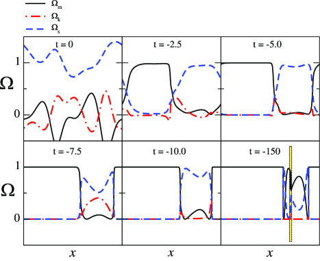
It is enlightening to visualize the evolution via the behavior of the matter ($\Omega_{m}$), shear ($\Omega_{s}$) and curvature ($\Omega_{k}$) contributions to the normalized energy density, defined as

$$\Omega_{m} \equiv {\textstyle{\frac{1}{6}}}{W^{2}}+{\textstyle{\frac{1}{6}}}{S^{\alpha}}{S_{\alpha}}+{\textstyle{\frac{1}{3}}}{\bar{V}}$$ (37)

$$\Omega_{s} \equiv {\textstyle{\frac{1}{6}}}{\Sigma^{\alpha\beta}}{\Sigma_{\alpha\beta}}$$ (38)

$$\Omega_{k} \equiv -{\textstyle{\frac{2}{3}}}{\kern-0.24994pt\hbox{$\partial$}\kern-5.30904pt\kern 0.50003pt\hbox{$\partial$}\kern-5.30904pt\kern-0.24994pt\raise 0.43304pt\hbox{$\partial$}_{\alpha}}{A^{\alpha}}+{A^{\alpha}}{A_{\alpha}}$$ (39)

$$+{\textstyle{\frac{1}{6}}}{N^{\alpha\beta}}{N_{\alpha\beta}}-{\textstyle{\frac{1}{12}}}{{({{N^{\gamma}}_{\gamma}})}^{2}},$$

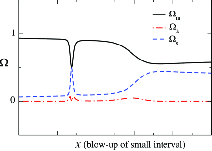
where $\Omega_{m}+\Omega_{s}+\Omega_{k}=1$ by (24). Fig.1 shows these quantities plotted at select times during the evolution (which was stopped at $t=-150$). Note that all features in the solution are locally smooth—apparent step functions in some of the plots are simply due to the large size of the domain relative to the size of the feature. As an example, Fig.2 shows a zoom-in of the last panel of Fig.1 about one of the late-time spike structures that formed in the anisotropic regime.

Figure 1: $t={\rm const.}$ snapshots of the normalized energy density in matter $\Omega_{m}$ (solid line), curvature $\Omega_{k}$ (dot-dash line) and shear $\Omega_{s}$ (dashed line) for $0\leq x\leq 2\pi$ at several times during the evolution of the initial data described in Sec.III. Time runs from left to right along the top row and continues along the bottom row. The shaded slit (dotted outline) in the last panel ($t=-150$) indicates the range of x shown in the blow-up in Fig.2.

Figure 2: Zooming in on one of the spike structures that formed in the anisotropic region at $t=-150$, as shown in Fig.1.

Figure 3: The effective equation of state parameter $w$ (40) for the simulation described in Sec.III, for $0\leq x\leq 2\pi$ at the same times as in Fig.1. At late times $w\rightarrow k^{2}/3-1$ in the matter dominated region, and $w\rightarrow 1$ in the anisotropic region (in this simulation $k=10$ for the potential (8)).

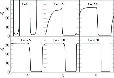
The effective equation of state parameter $w$ is shown in Fig.3, which takes the following form in Hubble normalized variables:

$$w=\frac{\frac{1}{2}W^{2}+\frac{1}{2}S^{\alpha}S_{\alpha}-\bar{V}}{\frac{1}{2}W^{2}+\frac{1}{2}S^{\alpha}S_{\alpha}+\bar{V}}.$$ (40)

By comparing Fig.1 and Fig.3 it is evident that at late times the region that has smoothed out and become matter dominated coincides with $w\gg 1$, whereas the anisotropic regime evolves to $w=1$ (and exactly so to within numerical truncation error).

The asymptotic behavior of the spacetime in the matter dominated region appears to coincide with that of a spacetime with an isotropic singularity in the sense of Goode and WainwrightGW . We therefore conjecture that in an ekpyrotic phase with an exponential potential, an open set of initial conditions leads to an isotropic singularity.

We can understand the behavior of the solution in the asymptotic matter dominated region by applying the following approximation which we expect to hold to arbitrary accuracy as the singularity is approached. To begin with, we neglect all spatial derivatives (such an approximation also holds in the anisotropic regions away from the isolated spikes). The constraint (24) then reduces to

$$\frac{W^{2}+2\bar{V}}{6}-1\approx 0,$$ (41)

and the slicing condition for ${\cal N}$ (13) becomes

$$3{\cal N}\approx\frac{3}{3-\bar{V}},$$ (42)

where we have used (41) to simplify the expression. We then assume that $\bar{V}$ remains finite and non-zero as the singularity is approached. This implies from (8,11,12) that $\phi$ takes the asymptotic form

$$\phi(x,t)\approx\phi_{0}(x)+\frac{2t}{k}$$ (43)

where $k$ is the constant in the expression for the potential $V=-{V_{0}}\exp(-k\phi)$. Thus $W$ (9) tends to

$$W\approx\frac{2}{k{\cal N}}.$$ (44)

Combining these relations gives

$$W \approx k,$$ (45)

$$\bar{V} \approx 3-\frac{k^{2}}{2},$$ (46)

$${\cal N} \approx \frac{2}{k^{2}},$$ (47)

and from (40)

$$w\approx k^{2}/3-1.$$ (48)

We conjecture that at the singularity the above approximations become exact, namely

$$\lim_{t\to-\infty}W = k,$$ (49)

$$\lim_{t\to-\infty}\bar{V} = 3-\frac{k^{2}}{2},$$ (50)

$$\lim_{t\to-\infty}{\cal N} = \frac{2}{k^{2}},$$ (51)

$$\lim_{t\to-\infty}w = k^{2}/3-1.$$ (52)

Our simulations support this conjecture in that at late times ($t=-150$ in this example) these quantities have, to within numerical truncation error, reached their limiting values. Detailed analysis of the asymptotic dynamics can be carried out following the method of Lim04 ; Coley04 ; Coley05 .

Fig.3 shows that as the singularity is approached the coordinate volumes of the $w=1$ vs. $w\gg 1$ regions of the universe are comparable. However, it turns out that the ratio of the proper volume of matter to anisotropic regions grows exponentially with time. Let $S$ denote the proper spatial volume element associated with the spatial metric $h_{ij}$ of $t={\rm const.}$ slices, i.e., $S=\sqrt{{\rm det}\ h}$. The fractional change of $S$ with respect to time is

$$\partial_{t}{\ln S}=-\frac{1}{2}h_{ij}\partial_{t}h^{ij},$$ (53)

which can be written as

$$\partial_{t}{\ln S}=3{\cal N}.$$ (54)

Thus the scale invariant lapse ${\cal N}$ is a direct measure of the rate at which the local proper volume element changes with time (and recall that $t\rightarrow-\infty$ as the singularity is approached). Fig.4 shows $3{\cal N}$ from the simulation at several times. In the asymptotic regime where spatial gradients are negligible, ${\cal N}$ approaches a constant (42), and thus (54) can be integrated to give

$$S_{m} \propto e^{6t/k^{2}},\ \ \ w\gg 1$$ (55)

$$S_{v} \propto e^{t},\ \ \ w=1$$ (56)

where we have used (42) where $w\gg 1$, and note that $\bar{V}\approx 0$ when $w=1$. Thus, at late times the ratio ${\cal R}$ of the proper volume of matter to anisotropic regions of the universe grows as

$${\cal R}=\frac{\int S_{m}dx}{\int S_{v}dx}\propto e^{-t(1-6/k^{2})}.$$ (57)

Thus, as long as $k>\sqrt{6}$ (which is equivalent to $w>1$), ${\cal R}\rightarrow\infty$ as $t\rightarrow-\infty$.

Figure 4: 3 times the scale invariant lapse ${\cal N}$ for the simulation described in Sec.III, for $0\leq x\leq 2\pi$ at the same output times as Figs.1 and 3.

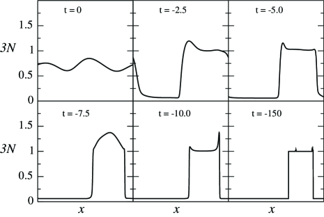
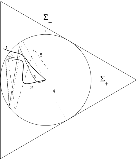
Fig.5 shows five state space orbits projected onto the $(\Sigma_{+},\Sigma_{-})$ plane, where

$$\Sigma_{+}=\frac{1}{2}(\Sigma_{11}+\Sigma_{22}),\quad\Sigma_{-}=\frac{1}{2\sqrt{3}}(\Sigma_{11}-\Sigma_{22}).$$ (58)

The orbits correspond to the evolution along the worldlines at $x=0,3.0,3.9,4.0,4.4$. All five orbits begin in the upper left quadrant, away from the origin, indicating anisotropic initial data. Towards the singularity, the first three orbits (solid lines) approach the origin of the plane, indicating isotropization. The fourth (dotted) and the fifth (dashed) do not isotropize.

Figure 5: The state space orbits for worldlines at $x=0,3.0,3.9,4.0,4.4$. Towards the singularity, the first three orbits (solid lines) approach the origin of the plane, indicating isotropization. The fourth (dotted) and the fifth (dashed) do not isotropize.

IV Conclusions

Our computations provide evidence that the ekpyrotic mechanism for smoothing and flattening the universe is robust and powerful, comparable qualitatively and quantitatively to the inflationary mechanism incorporated in the conventional big bang model. This evidence is the behavior as the singularity is approached of a class of spacetimes that, while not completely general, contain several degrees of freedom and begin far from FRW. Both the inflationary and the ekpyrotic mechanism require the addition of an energy component that is commonly mocked up as a scalar field with potential energy. For inflation, the important feature is that, for some initial conditions, the scalar field can act like a fluid with $w\approx-1$. It has been shown numerically that, beginning from highly non-linear and highly irregular initial conditions, regions dominated by the scalar field and with $w\approx-1$ come to dominate the volume of the universeGoldwirth . Similarly, we have found the regions in which the scalar field acts like a fluid with $w>1$ come to dominate exponentially the volume of the universe during a contracting phase.

This result addresses one of the key criticisms raised when the ekpyrotic model of the universe was first introduced; namely, it was suggested that the model required smooth initial conditions Kallosh:2001ai . One of the motivations for extending the ekpyrotic picture into a cyclic model was to include a period of dark energy domination before the ekpyrotic phase began in order to prepare smooth conditions Steinhardt:2002ih . Now, from the results here, it is clear that the dark energy epoch is not required for this purpose. Not only does this allow the possibility that the dark energy phase lasts only a few e-folds in the cyclic picture, as suggested in Erickson:2006wc , but it also opens the way for more general bouncing cosmologies that incorporate the ekpyrotic mechanism but do not cycle.

With these results in hand, we are now prepared to tackle the bounce itself in the case that it is non-singular ($a(t)$ shrinks to a non-zero value and then begins to increase). For the non-singular bounce, the equation of state must decrease from $w>1$ to $w<-1$ for a finite period during which anisotropy and inhomogeneity grows. Our goal is to determine if their growth can be kept at a level consistent with observations, establishing the viability of these bouncing cosmological models.

References

- (1) J. Khoury, B. A. Ovrut, P. J. Steinhardt and N. Turok, Phys. Rev. D 64, 123522 (2001)
- (2) J. K. Erickson, D. H. Wesley, P. J. Steinhardt and N. Turok, Phys. Rev. D 69, 063514 (2004).
- (3) E. I. Buchbinder, J. Khoury and B. A. Ovrut, Phys. Rev. D 76, 123503 (2007).
- (4) P. J. Steinhardt and N. Turok, Science 296, 1436 (2002).
- (5) see for example Sec. 8.6 of E.Kolb and M.S.Turner, The Early Universe, Addison-Wesley, Redwood City, CA. (1994)
- (6) D. S. Goldwirth, Phys. Rev. D43, 3204 (1991).
- (7) C. Uggla, H. van Elst, J. Wainwright and G. F. R. Ellis, Phys. Rev. D 68, 103502 (2003)
- (8) J. Curtis and D. Garfinkle, Phys. Rev. D 72, 064003 (2005)
- (9) M.J. Berger and J. Oliger, J. Comp. Phys. 53, 484 (1984)
- (10) F. Pretorius and M. W. Choptuik, J. Comput. Phys. 218, 246 (2006)
- (11) D. Garfinkle, Class. Quant. Grav. 21, S219 (2004)
- (12) A. A. Coley and W. C. Lim, Class. Quant. Grav. 22, 3073 (2005)
- (13) D. Garfinkle, Class. Quant. Grav. 24, S295 (2007)
- (14) D. Garfinkle and C. Gundlach, Class. Quant. Grav. 22, 2679 (2005)
- (15) J. W. York, Phys. Rev. Lett. 26, 1656 (1971)
- (16) B. K. Berger, D. Garfinkle, J. Isenberg, V. Moncrief, and M. Weaver, Mod. Phys. Lett. A13, 1565 (1998)
- (17) D. Garfinkle Phys. Rev. Lett. 93, 161101 (2004)
- (18) PAMR (Parallel Adaptive Mesh Refinement) and AMRD (Adaptive Mesh Refinement Driver) libraries (http://laplace.physics.ubc.ca/Group/Software.html)
- (19) H. Kreiss and J. Oliger, Global Atmospheric Research Programme, Publications Series No. 10. (1973)
- (20) A. Brandt, Math. Comput. 31, 333 (1977)
- (21) S. W. Goode and J. Wainwright, Class. Quant. Grav. 2, 99 (1985)
- (22) W. C. Lim, H. van Elst, C. Uggla and J. Wainwright, Phys. Rev. D 69, 103507 (2004)
- (23) A. A. Coley, Y. He and W. C. Lim, Class. Quant. Grav. 21, 1311 (2004)
- (24) R. Kallosh, L. Kofman and A. D. Linde, Phys. Rev. D 64, 123523 (2001)
- (25) J. K. Erickson, S. Gratton, P. J. Steinhardt and N. Turok, Phys. Rev. D 75, 123507 (2007)