Evolving Clustered Random Networks

Abstract

We propose a Markov chain simulation method to generate simple connected random graphs with a specified degree sequence and level of clustering. The networks generated by our algorithm are random in all other respects and can thus serve as generic models for studying the impacts of degree distributions and clustering on dynamical processes as well as null models for detecting other structural properties in empirical networks.

Empirical Network	$N$	$<d>$	$<d^{2}>$	$C$	$T$	$\tilde{C}$	$\tilde{T}$
Vancouver Urban Contacts	2627	13.9	265	0.07	0.09	0.09	0.14
WWW Subgraph	4271	4.2	119	0.09	0.01	0.15	0.08
Yeast Protein Interactions	4713	6.3	152	0.13	0.06	0.14	0.18
Astro-Phys Collaborations	5973	4.1	35	0.51	0.38	0.60	0.62
US Air Traffic	165	38.0	2765	0.86	0.58	0.97	0.96

Table 1: The number of nodes ($N$), the average node degree ($<d>$), the mean-squared of node degree ($<d^{2}>$), clustering coefficient ($C$), transitivity ($T$), Soffer-Vasquez clustering coefficient ($\tilde{C}$), and Soffer-Vasquez transitivity ($\tilde{T}$) for a set of empirical networks.

1 .  Introduction

Complex networks such as those formed by the links of the World Wide Web, social contacts between individuals in a city, and transportation routes have received much attention in the last decade. Recent studies have sought to characterize and explain non-trivial structural properties such as heavy-tail degree distributions, clustering, short average path lengths, degree correlations and community structure. These properties appear in diverse natural and manmade systems, and can fundamentally influence dynamical processes on these networks [41, 18, 29, 4, 8, 16, 2, 3].

Clustering, a property describing the presence of triangles in a network, is an important topological characteristic that can significantly impact dynamical processes over complex networks [41, 25, 34, 35, 30, 15]. It is often correlated with local graph properties such as correlations in the number of edges emanating from neighboring vertices [34], as well as global properties such as motifs [31, 39] and community structure [7].

Random graphs are graphs that are generated by some random process [26]. They are widely used as models of complex networks [29] and can assume various levels of complexity. The simplest model for generating random graphs, with only a single parameter, is the Bernoulli or Erdös-Renyi random graph model, which produces graphs that are completely defined by their average degree and are random in all other respects. A slightly more complex and general model is one that generates graphs with a specified degree distribution (or degree sequence) and are random in all other respects. These models can be extended to include additional structural constraints, such as degree correlations or the density of triangles or longer cycles. Here, we define a a random graph model which is constrained by the node degree distribution and the density of triangles in the graph.

1.1 .  Clustering in Real Networks

Clustering in real networks can stem from two sources: (a) it can arise as a byproduct of other, more fundamental, topological properties such as the degree sequence (distribution) or degree correlations; or (b) it can be generated directly by some inherent property or mechanism within the system, for example, “the friends of my friends tend to become my friends” in social networks.

Some researchers have claimed that high clustering is a general feature of complex networks [34]. When we measured clustering in a variety of empirical technological, biological and social networks, however, we found that it varies considerably. Table 1 shows that the clustering coefficients and transitivity values (a local and global measure of clustering, respectively) for these networks span the entire range of possible values (zero to one). Thus, it is important to understand not only the origins of clustering, but also the impact of clustering on network functions and dynamics. Towards this end, we introduce a method for generating random networks with a specified level of clustering.

1.2 .  Previous Work & Motivation

The study of clustering in complex networks began with the seminal work of Watts and Strogatz [41]. The authors presented a graph model with high clustering and low average path length, now known as the small-world property. Although not intended as a generative algorithm for clustered graphs, the model produces graphs with clustering spanning the range from 0 to 1. The graphs generated under this model, however, have rigid spatial structure and cannot accommodate varying degree distributions.

The first algorithms to explicitly generate graphs with a specified level of clustering for arbitrary degree distributions belonged to the class of projected bipartite graphs. Newman [25] introduced a three-step method that first builds a bipartite graph of individuals and affiliations, then projects the bipartite graph to a unipartite graph of individuals only, and finally runs a percolation process over the unipartite graph. This results in a clustered graph with a degree distribution that depends on the original distributions of numbers of individuals per group and groups per individual. The level of clustering in the final graph varies smoothly from 0 to 1 as a function of the percolation probability. In [11], Guillaume suggested a similar bipartite graph approach. Although these approaches can generate clustered graphs with diverse degree distributions, they lack straightforward methods for choosing parameters that yield graphs with not only a pre-specified clustering coefficient but also a pre-specified degree distribution. These algorithms also tends to produce disconnected graphs that leave a significant proportion of the graph vertices isolated.

A second class of clustered graph models use ”growing network“ algorithms [33, 40, 37]. The inputs to these models are a degree distribution and level of clustering. The method begins with a set of vertices with no edges; the graph is then “grown” by adding edges based on the degree and clustering constraints. Although the algorithms of this class allow for arbitrary degree distributions and levels of clustering, they either require a complex implementation [33], produce graphs of a highly specific structure [37] or introduce large amounts of degree correlations [37, 40].

Here, we present a model that generates simple and connected graphs with prescribed degree sequences and a specified frequency of triangles, while maintaining a graph structure that is as random (uncorrelated) as possible. There is an important difference between our model and previous work in the area. Prior models were intended to generate clustered graphs that replicate the properties of real-world networks; our goal is to generate a class of null networks with arbitrary degree distributions that are simple and connected and have a high density of triangles, but are random in all other respects.

Such a method is useful for two primary reasons: First, network structure fundamentally influences the functions of and dynamical processes on networks. We can use random clustered graphs to study the consequences of clustering, both independently and in combination with various degree patterns. Second, these networks can serve as null models for detecting whether an empirical network can be boiled down to its degree distribution and clustering values or, instead, contains substantial degree correlations or other important structures (beyond the byproducts of the degree distribution and clustering). One would first use the algorithm to generate an ensemble networks that match the empirical degree distribution and clustering values, and then compare the structural, functional, or dynamical properties of the empirical network to those of the random networks.

In Section 2, we review common measures of clustering and introduce our Markov chain model and algorithm for generating clustered graphs with a specified degree sequence. In Section 3, we test our algorithm with numerical simulations and discuss the structural properties of the generated graphs. Finally, in Section 4, we use the generated graphs to detect deviation from randomness in empirical networks.

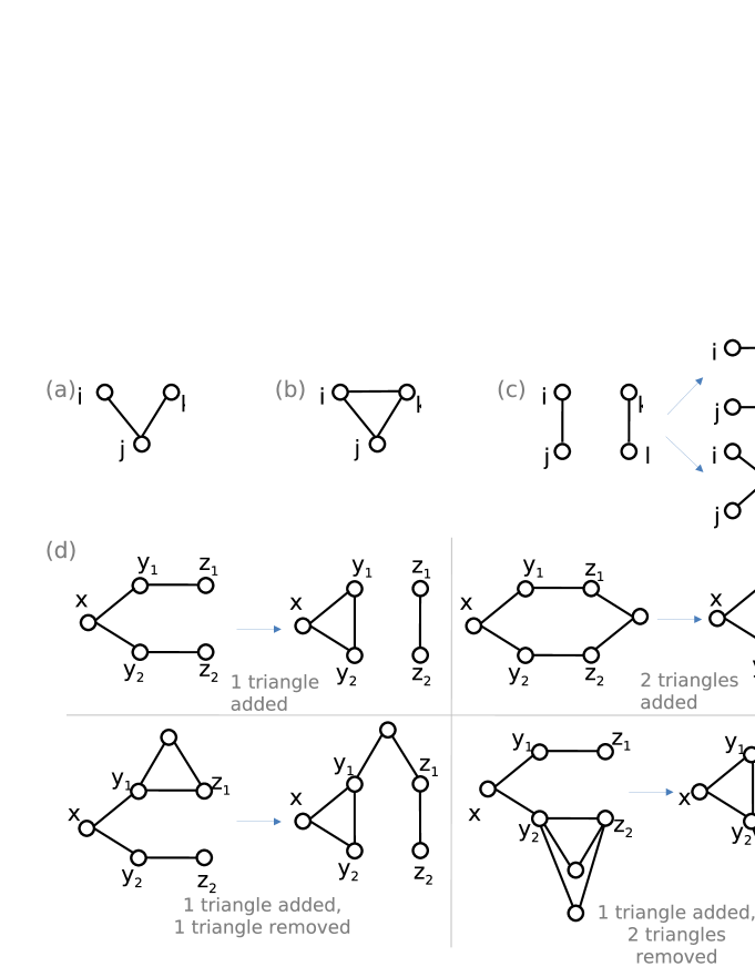
Figure 1: (a) a triple among the nodes $i,j,k$ (b) a triangle among the nodes $i,j,k$ (c) A rewiring of edges $(i,j)$ and $(k,l)$ can result in $(i,k)$ and $(j,l)$, or $(i,l)$ and $j,k)$ (d) Four (among many) scenarios for the result of one rewiring step of our algorithm. The configuration of edges before (left) and after (right) a rewiring step are shown for each scenario. The two bottom scenarios would be rejected by our algorithm as they do not strictly increase the number of triangles.

2 .  Methods and Model

Our random graph generation method begins with a random graph and iteratively rewires edges to introduce triangles. Network rewiring is a well-known method for generating networks with desired properties [19]. Two edges are called adjacent if they connect to a common node. Each rewiring is performed on two non-adjacent edges of the graph and consists of removing these two edges and replacing them with another pair of edges. Specifically, a pair of edges $(i,j)$ and $(k,l)$ is replaced with either $(i,k)$ and $(j,l)$, or $(i,l)$ and $(j,k)$ (as illustrated in Figure 1c). This change in the graph leaves the degrees of the participating nodes unchanged, thus maintaining the specified degree sequence. Below we describe a rewiring algorithm that increases the level of clustering in a random graph, while preserving the degree sequence.

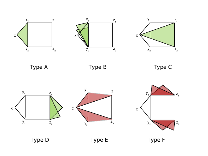
Figure 2: Possible triangle additions (green) and removals (red) in one step of the rewiring procedure. Black lines represent existing edges and edges added after a rewiring event, gray lines represent edges lost during a rewiring event.

2.1 .  Measures of Clustering

We begin with a graph $G=(V,E)$ which is undirected and simple (no self-loops or multiple edges). $V$ is the set of vertices of $G$ and $E$ is the set of the edges. We let $N=|V|$ and $M=|E|$ denote the number of nodes and edges in $G$, respectively. The degree of a node $i$ will be denoted $d_{i}$. The set of degrees for all nodes in the graph makes up the degree sequence, which follows a probability distribution called the degree distribution.

Clustering is the likelihood that two neighbors of a given node are themselves connected. In terms of social networks, it measures the probability that “the friend of my friend is also my friend.” In topological terms, clustering measures the density of triangles in the graph, where a triangle is the existence of the set of edges ${(i,j),(i,k),(j,k)}$ between any triplet of nodes $i,j,k$ (Figure 1b).

To quantify the local presence of triangles, we define $\delta(i)$ as the number of triangles in which node $i$ participates. Since each triangle consists of three nodes, it is counted thrice when we sum $\delta(i)$ for each node in the graph. Thus the total number of triangles in the graph is

$$\delta(G)=1/3\sum_{i\in V}\delta(i).$$

A triple is a set of three nodes, $i,j,k$ that are connected by edges $(i,j)$ and $(j,k)$, regardless of the existence of the edge $(i,k)$ (Figure 1a). The number of triples of node $i$ is simply $\tau(i)=\left(\begin{array}[]{c}d_{i}\\ 2\end{array}\right)$, assuming $d_{i}\geq 2$. To compute the total number of triples in the graph we sum $\tau(i)$:

$$\tau(G)=\sum_{i\in V}\tau(i).$$

The term triadic closure refers the conversion of a triple into a triangle via the addition of a third edge [INSERT REFS].

The clustering coefficient was introduced by Watts and Strogatz [41] as a local measure of triadic closure. For a node $i$ with $d_{i}\geq 2$, the clustering coefficient $c(i)$ is the fraction of triples for node $i$ which are closed, and can be measured as $\delta(i)/\tau(i)$. The clustering coefficient of the graph is then given by:

$$C(G)=\frac{1}{N_{2}}\sum_{\{i\in V|d_{i}\geq 2\}}c(i),$$

where $N_{2}$ is the number of nodes with $d_{i}\geq 2.$

A more global measure of the presence of triangles is called the transitivity of graph $G$ and is defined as:

$$T(G)=\frac{3\delta(G)}{\tau(G)}.$$

Although they are often similar, $T(G)$ and $C(G)$ can vary by orders of magnitude [35]. They differ most when the triangles are heterogeneously distributed in the graph.

These traditional measures of clustering are degree-dependent and thus can be biased by the degree sequence of the network. The maximum number of possible triangles for a given node $i$ is just its number of triples ($\tau(i)$). For a node which is connected to only low degree neighbors, however, the maximum number of possible triangles may be much smaller than $\tau(i)$. To account for this, a new measure for clustering was introduced in [35] that calculates triadic closure as a function of degree and neighbor degree. Specifically, the Soffer-Vasquez clustering coefficient ($\tilde{C}$) and transitivity ($\tilde{T}$) are given by:

$$\tilde{C}=\frac{\sum_{i|\omega_{i}>0}\delta(i)/\omega(i)}{N_{\omega}}$$

$$\tilde{T}=\frac{\sum_{i}\delta(i)}{\sum_{i}\omega(i)},$$

where $\omega(i)$ measures the number of possible triangles for node $i$, and $N_{\omega}$ is the number of nodes in $G$ for which $\omega(i)>0$. We note that $\tilde{C}$ and $\tilde{T}$ are undefinited if $\omega(G)=\sum_{i}\omega(i)=0$. $\omega(i)$ is computed by counting the maximum number of edges that can be drawn among the $d_{i}$ neighbors of a node $i$, given the degree sequence of $i$’s neighbors; this value is often smaller than $\left(\begin{array}[]{c}d_{i}\\ 2\end{array}\right)$ [35]. For example, consider a star network of five nodes, where four nodes have degree 1 and one node has degree 4. Although the total number of triples is $\tau(G)=6$, the number of possible triangles is $\omega(G)=0$ because the degree one nodes preclude their formation.

2.2 .  Generating Random Graphs

Generating random graphs uniformly from the set of simply connected graphs with a prescribed degree sequence is a well-studied problem with algorithmic solutions [19]. One of the simplest and most popular of these generative algorithms was originally suggested by Molloy and Reed [20]. Their model, however, sometimes produces graphs that are not simple or connected. This can be remedied by subsequently removing multiple edges and self loops from the constructed graph and keeping only the largest connected component. Although this approach works, the Markov Chain Monte Carlo (MCMC) method for generating simple connected graphs with specified realizable degree sequences [1, 6] presented in [9, 19] is less prone to problems. It proceeds as follows:

1. Create a graph with the desired degree sequence using the deterministic Havel-Hakimi algorithm. [14, 12].

2. Connect any disconnected components of the graph using the Taylor algorithm [36].

3. Randomly rewire the graph while keeping it simple and connected [19].

The Havel-Hakimi algorithm is iterative and tracks the residual degree of each node, which is the difference between its current degree and desired degree. In each iteration, it picks an arbitrary node $x$ and adds edges from $x$ to $d_{x}$ other nodes with the highest residual degrees, where $d_{x}$ is the degree of $x$. The residual degrees of all the nodes are then updated. The Taylor algorithm merges disconnected components of a graph by randomly selecting edges $(i,j)$ and $(k,l)$ from different components of the graph and rewiring them to $(i,k)$ and $(j,l)$, as long as the rewiring does not create new disconnected components.

2.3 .  Markov Chain Model

Our method of generating clustered graphs can be described by a Markov chain. We let $D$ be a realizable degree sequence and define $G_{D}$ to be the set of all simple, connected graphs with degree sequence $D$. If $G_{1},G_{2},...,G_{|G_{D}|}$ are the graphs of $G_{D}$, then we let $X_{1},X_{2},...,X_{|G_{D}|}$ be the states of the Markov chain, $P$, where $X_{i}$ represents the state in which our graph $G=G_{i}$. The states $X_{i}$ and $X_{i+1}$ are connected in the Markov Chain if $G_{i}$ can be changed to $G_{i+1}$ with the rewiring of one pair of edges. The state space of the Markov chain $P$ is connected because there exists a path from $X_{i}$ to $X_{j}$ (for any pair $i,j$) by one or more rewiring moves that leave the degree sequence unchanged [36].

Our clustered graph generation algorithm involves first obtaining a graph, $G$ of $G_{D}$ by the method outlined in Section 2.2, and then transitioning from the state corresponding to $G$ ($X_{G}$) to other states of $P$ until a halting condition is reached. A transition from one state of the Markov chain to another only happens when the algorithm makes an edge rewiring that both increases the number of triangles in the graph and leaves the graph connected. Since a rewiring does not alter the degree sequence of the graph, the rewired graph is still in $G_{D}$. The transition probabilities of the Markov chain for a pair of connected states, $X_{i}$ to $X_{j}$, are:

$$P_{ij}=\left\{\begin{array}[]{ll}1&\mbox{if $(\Delta_{j}-\Delta_{i})>0$ and $G_{j}$ is connected}\\ 0&\mbox{otherwise}\\ \end{array}\right.$$

where $\Delta_{i}$ is the number of triangles in $G_{i}$. The algorithm continues searching for a feasible rewiring (one that increases the number of triangles and does not disconnect the graph) until one is found. If a feasible move is not found, a transition is not made and the process remains in the current state.

The Markov chain above is finite and aperiodic, but not irreducible as the process can never transition to a state in which the graph has fewer triangles. It does, however, have an absorbing state, $X_{*}$, in which the transitivity of $G_{*}$ is greater than or equal to the desired transitivity or is the maximum possible transitivity given the particular degree sequence and connectivity constraints.

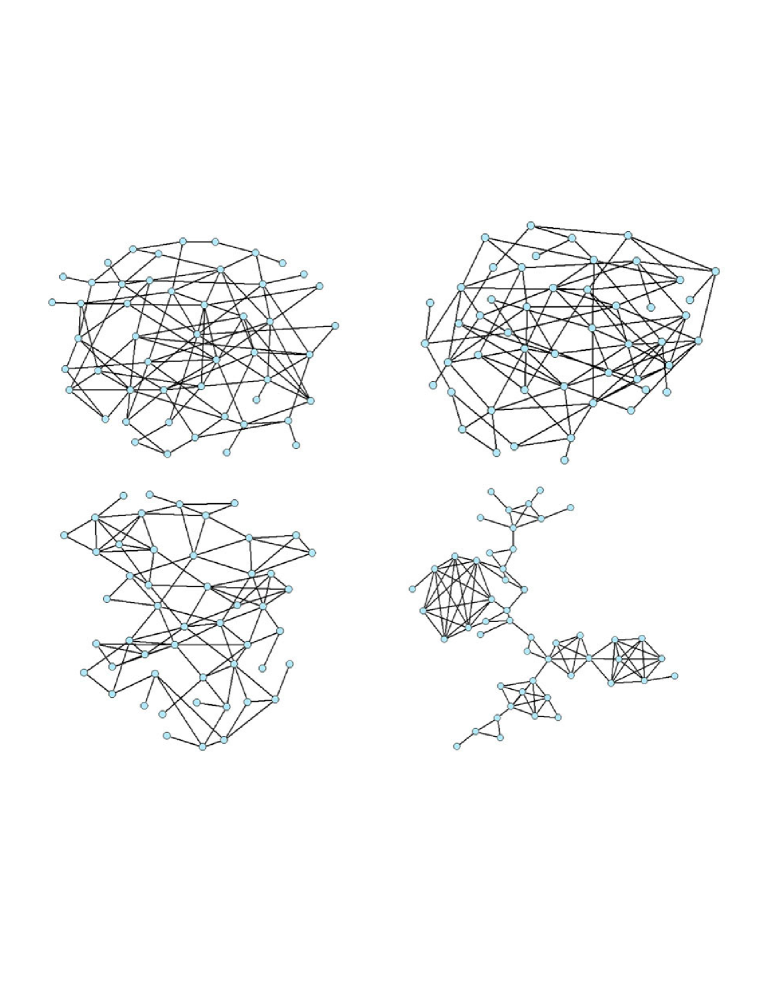
Figure 3: The evolution of the graph from (a) $\tilde{T}\approx 0$ ,(b) $\tilde{T}=0.1$,(c) $\tilde{T}=0.5$ and (d) $\tilde{T}=0.8$ [10]

2.4 .  Algorithm

Our Markov Chain simulation algorithm for generating clustered random graphs is described below and illustrated in Figure 1d.

Input: A random graph, $G$, with a realizable degree sequence $\{d_{i}\}$, generated using the method outlined in Section 2.2 or another suitable method, a desired clustering value, $target$, and a tolerance value TOL.

Initialization: Measure the clustering of $G$, $clust(G)$.

while $|clust(G)-target|\geq$ TOL do  1. uniformly select a random node, $x$, from the

set of all nodes of $G$ such that $d_{x}>1$.

uniformly select two random neighbors, $y_{1}$

and $y_{2}$, of $x$ such that $d_{y_{1}}>1$ and

$d_{y_{2}}>1$ and $y_{1}\neq y_{2}$.

uniformly select a random neighbor, $z_{1}$

of $y_{1}$ and a random neighbor, $z_{2}$ of

$y_{2}$ such that $z_{1}\neq x$, $z_{2}\neq x$,

$z_{1}\neq z_{2}$.

$G_{cand}:=G$ where $G_{cand}$ is the candidate

graph to which the transition may be made.

if $(y_{1},y_{2})$ and $(z_{1},z_{2})$ do not exist then  Rewire two edges of $G_{cand}$: delete $(y_{1},z_{1})$ and $(y_{2},z_{2})$, add $(y_{1},y_{2})$ and $(z_{1},z_{2})$. end

Update the value of $clust(G_{cand})$ by measuring

$\delta(i)$ (and $\omega(i)$ if relevant) for the nodes involved

in the rewiring and their neighbors.

if $clust(G_{cand})>clust(G)$ and $G_{cand}$

is connected then  $G:=G_{cand}$ end end Output: A random graph, $G$ with degree sequence $\{d_{i}\}$ and $clust(G)=target\pm$TOL.

The algorithm terminates when the desired clustering (within a given tolerance) or the maximum clustering possible is reached. In the latter case, the desired clustering is not achieved given the degree and connectivity constraints. Theoretically, the algorithm may never reach the target, but if it does, the answer is guaranteed to be correct (this is also sometimes known as a Las Vegas type algorithm). For practical implementation purposes, a threshold can be placed on the number of iterations run by the algorithm in the case that the desired clustering cannot be reached.

2.4.1 Choice of Clustering Measure

The algorithm is defined independent of the choice of clustering measure. The term $clust(G)$ in the algorithm above can be replaced by any clustering measure described in Section 2.1, or, more simply, the number of triangles in the graph.

The choice of clustering measure does, however, affect the output of the algorithm. The clustering coefficient is a local measure; and thus $C$ and $\tilde{C}$ yield networks that are only locally optimized for the desired level of clustering. Also, as connectivity is required by our algorithm, the algorithm does not generate graphs which must be disconnected into multiple components to attain high levels of clustering. (An example of this is given in Appendix Figure 8). The algorithm may also have difficulty attaining target clustering values when using the standard clustering measures ($C$ or $T$) because of joint degree constraints (the degrees of adjacent nodes) on the possible numbers of triangles, as with the example presented in Section 2.1. The Soffer-Vasquez clustering measures, which explicitly consider joint degree constraints, provide a way around this difficulty [35]. Although the rewiring in our algorithm changes the joint degree distribution (and thus the degree correlations) of the graph, $\omega(G)$ is not altered significantly during network generation (as shown in Appendix Figure 9). Thus, when using $\tilde{C}$ or $\tilde{T}$, clustering is increased primarily by the addition of triangles (that is, increasing $\delta(G)$) rather than decreasing $\omega(G)$).

Generated Network Type	$N$	$<d>$	$<d^{2}>$	$T$	$\tilde{T}$	$Diam$	$r$	$Q$
Vancouver Urban Contacts	2627	13.9	265	0.09[0]	0.14 [0]	6 [0]	0.15 [-0.4]	0.28 [-0.15]
WWW Subgraph	4271	4.2	119	0.03 [0.02]	0.1 [0.02]	15 [5]	0.07[0.37]	0.45[-0.15]
Yeast Protein Interactions	4713	6.3	152	0.07[0.01]	0.18 [0]	12.5 [3.5]	0.11 [0.07]	0.39 [-0.1]
Astro-Phys Collaborations	5973	4.1	35	0.26[-0.05]	0.62[0]	17 [-3]	0.25 [-0.07]	0.70[-0.1]
US Air Traffic	165	38.0	2765	0.58[0]	0.97 [0]	3 [0]	-0.55 [0]	0.11 [-0.01]

Table 2: Comparisons between empirical networks and random graphs. For each empirical network, we generated 25 random graphs constrained to have the observed degree sequences and Soffer-Vasquez transitivity values. The table reports average values of several network statistics for the random graphs: network size ($N$), mean degree ($\langle d\rangle$), mean squared degree ($\langle d^{2}\rangle$), Soffer-Vasquez clustering coefficient ($\tilde{C}$), Soffer-Vasquez transitivity ($\tilde{T}$), maximum shortest path length between any two nodes ($diam$), degree correlation coefficient ($r$), and modularity ($Q$). The value given in brackets is the deviation of the ensemble mean from the corresponding statistic for the empirical network. (A positive relative deviation indicates that the ensemble mean was greater than the empirical statistic and vice versa.) Deviations are not listed for $N$, $\langle d\rangle$ and $\langle d^{2}\rangle$ as network size and degree sequence are constrained by our algorithm to match the empirical networks perfectly.

2.5 .  Analysis

As shown in Figure 2, there are six types of triangles that can be added or removed for every pair of edges that are rewired. As illustrated in Figure 1d, these additions and removals can occur in combination.

Type A: The addition of the edge between vertices $y_{1}$ and $y_{2}$ guarantees the addition of one triangle in every rewiring event.

Type B: The addition of the edge $(y_{1},y_{2})$ could create new triangles with shared neighbors of $y_{1}$ and $y_{2}$.

Type C: The addition of the edge $(z_{1},z_{2})$ could add a triangle if there existed edges between $x$ and $z_{1}$ and $x$ and $z_{2}$.

Type D: The addition of the edge between vertices $z_{1}$ and $z_{2}$ could create new triangles with shared neighbors of $z_{1}$ and $z_{2}$.

Type E: The removal of edges $(y_{1},z_{1})$ and $(y_{2},z_{2})$ removes one triangle each if the edges $(x,z_{1})$ or $(x,z_{2})$ exist.

Type F: The removal of the edges between vertices $y_{1}$ and $z_{1}$, and $y_{2}$ and $z_{2}$ could lead to the removal of existing triangles with shared neighbors of $y_{1}$ and $z_{1}$ or $y_{2}$ and $z_{2}$.

We note that although the type A addition is a special case of type B, the type C addition is a special case of type D, and the type E removals are a special case of type F, we distinguish them because they have different probabilities of occurrence. Our look-ahead strategy only allows rewiring moves when the total number of Type E and F losses is fewer than the total number of Type A, B, C, and D gains.

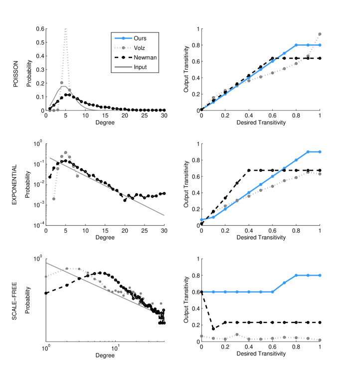
Figure 4: Discrepancies between input and output degree distributions (left panels) and transitivity values (right panels) for an ensemble of 15 Poisson (top panels), exponential (middle panels) and scale-free graphs (bottom panels) as generated by our algorithm and the algorithms presented in [40] and [25]. Each graph has $N=500$ and mean degree, $\langle d\rangle=5$. The input degree distribution is shown as a gray solid line (left graphs); and output degree distributions are not shown for our algorithm as they always perfectly match the input. The input and output transitivity values are measured as $\tilde{T}$ for our algorithm, and as $T$ for the Volz and Newman algorithm.

2.6 .  Computational Complexity

Like many MCMC methods, the algorithm we propose can be computationally expensive. The method outlined in Section 2.2 requires $O(M)$ steps to generate a connected graph, and up to $O(M)$ steps to randomize the graph, where $M$ is the number of edges in the graph. At each step of randomization, we test that the graph remains connected (an $O(M)$ operation), resulting in an overall $O(M^{2})$ network generation process. A naive computation of the transitivity/clustering coefficient requires checking every node for the existence of edges between every pair of neighbors of the node. This step requires $O(Nd_{max}^{2})$ operations, where $N$ is the number of nodes and $d_{max}$ is the maximum degree of any node in the graph.

The most expensive step of our algorithm is the introduction of triangles via rewiring. A single rewiring step requires $O(M)$ operations for switching edges, checking for connectivity and updating the triangle count. Although we cannot calculate analytically the number of rewiring steps required to reach the desired transitivity, we have found it empirically to be $O(M)$. Thus, the average complexity of the algorithm presented here is $O(M^{2})$. This complexity has been computed for the most naive versions of our algorithms; and more efficient implementations may improve the complexity greatly. For example, we might improve efficiency by performing connectivity tests once every $x$ rewirings (for some number $x$) rather than during every rewiring, as proposed in [9].

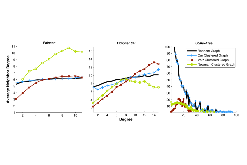
Figure 5: Degree correlations in random graphs with specified degree distributions (Poisson, exponential and scale-free with mean degree = 5) compared to clustered random graphs with the same degree distributions and $\tilde{T}=0.5$ generated by our algorithm and the Volz [40] and Newman [25] algorithms. The graphs present averages over 15 graphs generated by each algorithm. Our algorithm introduces fewer degree correlations than the alternatives.

3 .  Results

3.1 .  Numerical Simulations

To check the feasibility and reliability of the algorithm, we generated networks for several degree distributions and a range of clustering values. Specifically, we used Poisson $\left(p_{d}=e^{-\lambda}\lambda^{d}/d!\right)$, exponential $\left(p_{d}=(1-e^{\kappa})e^{-\kappa(d-1)}\right)$ and scale-free $\left(p_{d}=d^{-\gamma}/\zeta(\gamma)\right)$ degree distributions, and Soffer-Vasquez transitivity ($\tilde{T}$) ranging from 0 to 1 in increments of 0.1. Figure 3 illustrates a graph (N=50) with a Poisson distributed degree sequence evolving towards higher transitivity.

We evaluated the performance of the algorithm in comparison to those proposed in [40] (as a representative of the growing networks class of clustered graphs generators) and in [25] (as a representative of the class of bipartite models). Specifically we measured the discrepancies between input and output degree distributions (Figure 4, left graphs) and transitivity values (Figure 4, right graphs). Our algorithm preserves the input degree sequence perfectly, while there are considerable mismatches between the input and output degree distributions in the Volz and Newman models. For Poisson and exponentially distributed graphs, our algorithm closely approaches the target transitivity. These degree distributions cannot, however, reach the highest transitivity values (Figures 4b and 4d) without disconnecting the graph. Unlike our algorithm, the Volz and Newman models do not require connectivity, which may explain the superior performance of the Volz algorithm on the Poisson network at the maximum transitivity value (Figure 4b). The Volz algorithm also performs well at low values of $T$ for both the Poisson and exponential networks (Figures 4b and 4d); while the Newman algorithm only performs well on the Poisson networks.

Our algorithm performs quite poorly on scale-free random graphs (Figure 4f), which have much higher clustering a priori than expected for Poisson random graphs [34, 28]. Our algorithm is not designed to decrease clustering, and therefore can only reach the desired level if the initial random graph has lower clustering than desired. The triangles in a connected scale-free random graph are also close to the minimum required to keep the graph connected, and thus, modifying our algorithm to decrease (as well as increase) the triangles in a graph would likely not improve its performance on the scale-free graphs.

3.2 .  Structural Properties of Our Generated Networks

There are several other topological properties (besides degree sequence and transitivity) that can strongly influence network function and dynamics: degree correlations (the dependence of a node’s degree on its neighbor’s degrees), community structure (groups of nodes that are highly intra-connected and only loosely inter-connected), and average path length (typical distances between pairs of nodes in the network). We have specifically developed this model to increase clustering with minimal structural byproducts. Thus, we confirm that we have reached this goal by measuring the above properties in the networks generated by our algorithm.

We evaluated the extent to which the algorithm introduces degree correlations by comparing random (unclustered) graphs to clustered random graphs generated by our algorithm and the Volz [40] and Newman [25] algorithms (Figure 5). While our algorithm essentially preserves the correlation structure of the random graph, the other algorithms produce highly correlated graphs.

Several authors have discussed the relationship between clustering and community structure [28, 7, 32, 34]. As Figure 3 shows, the addition of triangles leads to modular structure. This behavior is not surprising: as the number of edges in the graph is constrained, sets of connected nodes with high $\omega(i)$ values (often high-degree nodes) must be brought together to create additional clustering.

Short average path lengths are a characteristic feature of random graphs [23]. To quantify the impact of our algorithm on path lengths, we calculated the average path length for each node to all other $(N-1)$ nodes, and then compared the distributions of these values for several random and random clustered graphs (Figure 6). While our algorithm preserves short average path lengths, the mean of the path length distribution tends to be slightly larger for the clustered graphs than for the corresponding random graphs. The intuition behind this increase in average path length may lie in the increased community structure: as graphs become more clustered and separate into subgroups, nodes in different groups require more links to reach each other.

Figure 6: Average path lengths in random graphs with specified degree distributions (Poisson and exponential with mean degree = 5) compared to clustered random graphs with the same degree distributions and $\tilde{T}=0.5$ generated by our algorithm. The histograms are based on 15 networks of each type. The clustered graphs have slightly higher means than their random counterparts: 4.05 for the Poisson random graphs verus 4.39 for the clustered graphs; and 3.95 for the exponential random graphs versus 4.14 for the custered graphs.

3.3 .  Comparison to Empirical Networks

Our algorithm can also be applied to detecting non-random structure in empirical networks. We can generate ensembles of clustered random networks with empirically estimated degree distributions and clustering values to ascertain whether empirical networks have significant non-random structure in other respects. We demonstrate this application using representatives from five different classes of real networks: (1) a social network, made up of contacts between individuals in the city of Vancouver [18], (2) a protein interaction network for yeast [38], (3) a technological network, made up of a subset of the links of the World Wide Web [17], (4) a transportation network, made up of US metropolitan areas connected by air travel [5], and (5) a collaboration network, made up of scientists connected by coauthorship on scientific preprints on the Astrophysics E-Print Archive between 1995 and 1999 [22], with a collaboration strength of 0.5 or greater [21]. The basic statistics of these networks, including clustering values, are listed in Table 1.

We used the following method to quantify deviations from randomness in these networks. First, we used our algorithm to generate 25 clustered random networks constrained to match the empirical degree distribution and clustering values. Second, we selected a set of network topological measures (other than degree distribution and clustering), and compared these quantities for the empirical graph to the corresponding average quantities across the ensemble of generated graphs.

Specifically, we generate 25 random clustered networks for each empirical network, constrained to match the empirical degree sequence and Soffer-Vasquez transitivity. In addition to the degree and clustering metrics, we also calculated diameter (longest shortest path length between any pair of nodes in the graph) [13], degree correlation coefficient [24] and modularity (degree of community structure) [27] (Table 2). Other than diameter, each of these range from 0 to 1. The standard deviations for all statistics are negligible and thus not reported. For every statistic, we also give the deviation between the empirical value and the average across the generated ensemble of random clustered networks (specifically, deviation = ensemble mean - observed value). Small deviations suggest that the empirical network structure boils down to the degree distribution and clustering, and thus we turn our attention to possible mechanisms underlying these properties. In contrast, large deviations suggest that there are other fundamental properties to consider in addition to or, perhaps, instead of clustering.

The random counterparts of the US air traffic network, for example, have structural properties almost identical to the real network, suggesting that the structure of the US air traffic network comes almost exclusively from its degree patterns. (In fact, even the high clustering is explained exclusively by the degree patterns.) We note that the US air traffic network is the most engineered of the networks we consider, and thus may have fewer emergent properties. The remaining empirical networks differ considerably from their random counterparts, suggesting that there are important mechanistic features not captured in our random model. For example, the two social networks (the Vancouver urban contact network and the Astro-Phys collaboration network) have higher degree assortativity than our random networks. This may point to rules of social behavior beyond that dictated by number of “friends” and the tendency that “my friend’s friend is also my friend.” All the natural networks also have significantly higher community structure than the corresponding random networks, inspite of having a wide range of transitivity values. This shows that clustering and community structure are not necessarily postively correlated.

4 .  Conclusion

In this work, we have introduced a Markov chain simulation algorithm to generate clustered random graphs with a specified degree sequence and level of clustering. Our algorithm perfectly preserves the degree sequence of a random graph and generally maintains other fundamental properties of random graphs like short path length and low degree correlations. An ensemble of the graphs generated by this algorithm can thus be useful for systematically studying the impact of triangles on network function and dynamics and understanding identifying the essential structural features of empirical networks. Since this method is based on a dynamic process, it can be used to generate both static networks with a specified amount of clustering and dynamic networks with evolving levels of clustering. Furthermore, since the process is a “memoryless” one, additional clustering can be added to any network without having to grow a new one from scratch.

Appendix

We evaluated the effectiveness of an algorithm which accepts all rewirings regardless of their effect on the number of triangles. Recall that our main algorithm only makes rewirings that increase the number of triangles. In Figure 7, we show that the permissive algorithm is not effective in achieving the desired levels of clustering. Additionally, other structural properties of the network, e.g. degree correlations, are significantly altered from the orginal graph in this case (as shown in the right panel of Figure 7.)

Figure 8 illustrates a network in which disconnection is required to achieve maximal clustering.

Figure 9 shows that our algorithm does not change the number of possible triangles ($\omega(G)$) in the graph drastically.

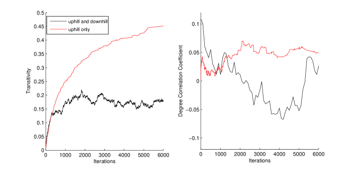
Figure 7: The effect of allowing both uphill (rewirings that increase the total number of triangles) and downhill (rewirings that decrease the total number of triangles) moves. These results are shown for a Poisson distributed graph of 500 nodes. In the left panel, we see that allowing all rewirings is not effective in reaching the desired transitivity ($T=0.45$). We also find that the structure of the graph is altered significantly in the process of making all rewirings. The degree correlation coefficient, for example, varies significantly with each rewiring (as shown in the right panel.

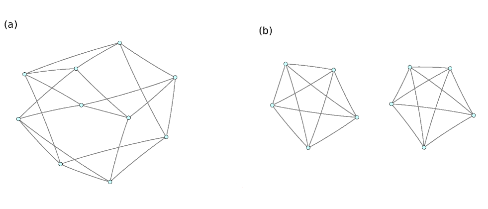
Figure 8: (a) A random graph with 10 nodes, each of degree 4. (b) The graph in (a) must be disconnected to be maximally clustered ($C=T=\tilde{C}=\tilde{T}=1$).

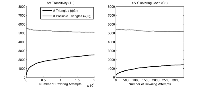
Figure 9: The numbers of triangles $\delta(G)$ and possible triangles $\omega(G)$ in the graph as the algorithm progresses. $\omega(G)$ does not vary substantially during graph generation. These results are for a Poisson distributed graph of 500 nodes, to which triangles are added until reaching (a) Soffer-Vasquez transitivity = 0.5 and (b) Soffer-Vasquez clustering coefficient = 0.5.

References

- [1] A realizable degree sequence is one which satisfies the handshake theorem (the requirement that the sum of the degrees be even) and the erdos-gallai criterion (which requires that for each subset of the highest degree nodes, the degrees of these nodes can be “absorbed” within the subset and the remaining degrees.
- [2] R. Albert and A. L Barabasi. Statistical mechanics of complex networks. Reviews of Modern Physics, 74:47–97, 2002.
- [3] R. Albert, H. Jeong, and A. L Barabasi. Error and attack tolerance of complex networks. Nature, 406:378–382, 2000.
- [4] R. Albert, H. Jeong, and A.L Barabasi. Diameter of the world-wide web. Nature, 401:130–131, 1999.
- [5] US Bureau of Transportation Statistics. http://www.transtats.bts.gov/,.
- [6] P. Erdos and T. Gallai. Graphs with prescribed degree of vertices. Mat. Lapok., 11:264–274, 1960.
- [7] F. Cecconi V. Loreto F. Radicchi, C. Castellano and D. Parisi. Defining and identifying communities in networks. PNAS, 1019, 2004.
- [8] M. Faloutsos, P. Faloutsos, and C. Faloutsos. On power-law relationships of the internet topology. Proceedings of the Conference on applications, technologies, architectures, and protocols for computer communications., pages 251 – 262, 1999.
- [9] C. Gkantsidis, M. Mihail, and E. Zegura. The markov chain simulation method for generating connected power law random graphs. Proc. 5th Workshop on Algorithm Engineering and Experiments (ALENEX.SIAM), 2003.
- [10] the Network Analysis Package Graphs were produced using Pajek.
- [11] J. Guillaume and M. Latapy. Bipartite graphs as models of complex networks. Lecture Notes in Computer Science, 3405:127–139, 2005.
- [12] S.L Hakimi. On the realizability of a set of integers as degrees of the vertices of a liinear graph. SIAM Journal, 103:496–506, 1962.
- [13] F Harary. Graph Theory. Oxford University Press, London, 1969.
- [14] V. Havel. A remark on the existence of finite graphs. Caposis Pest. Mat., 80:496–506, 1955.
- [15] M.J Keeling. The effects of local spatial structure on epidemiological invasions. Proc. R. Soc. B, 266:859–867, 1999.
- [16] M.J. Keeling and K.T.D Eames. Networks and epidemic models. J. R. Soc. Interface, 2:295–307, 2005.
- [17] Pages linking to www.epa.gov. http://www.cs.cornell.edu/courses/cs685/2002fa/.
- [18] L.A. Meyers, B. Pourbohloul, M.E.J. Newman, D.M. Skowronski, and R.C Brunham. Network theory and sars: predicting outbreak diversity. J. Theo. Biol, 232:71–81, 2005.
- [19] R. Milo, N. Kashtan, S. Itzkovitz, M.E.J Newman, and U Alon. Subgraphs in networks. Phys Rev E, 70(058102), 2004.
- [20] M. Molloy and B. 1995 Reed. A critical point for random graphs with a given degree sequence. Random Struct. Algo, 6(161).
- [21] M.E.J. Newamn. Scientific collaboration networks: Ii. shortest paths, weighted networks, and centrality. Phys. Rev. E, 016132, 2001.
- [22] M.E.J. Newamn. The structure of scientific collaboration networks. PNAS, 98, 2001.
- [23] M. E. J. Newman, S. H. Strogatz, and D. J. Watts. Random graphs with arbitrary degree distributions and their applications. Phys. Rev. E, 64:026118, 2001.
- [24] M.E.J Newman. Assortative mixing in networks. Phys. Rev. Lett, 89, 2002.
- [25] M.E.J Newman. Properties of highly clustered networks. Phys. Rev. E, 68(026121), 2003.
- [26] M.E.J. Newman. Random graphs as models of networks. Handbook of Graphs and Networks, 2003.
- [27] M.E.J. Newman. Detecting community structure in networks. Eur. Phys. J. B, 38:321–330, 2004.
- [28] M.E.J. Newman and J. Park. Why social networks are different from other types of networks. Phys. Rev. E, 68(036122), 2003.
- [29] M.E.J. Newman, D.J. Watts, and S.H. Strogatz. Random graph models of social networks. Proc. Natl. Acad. Sci., 99(2566), 2002.
- [30] T. Petermann and P.D.L Rios. The role of clustering and gridlike odering in epidemic spreading. Phys Rev E, 69(066116), 2004.
- [31] S. Itzkovitz N. Kashtan D. Chklovskii R. Milo, S. Shen-Orr and U. Alon. Network motifs: Simple building blocks of complex networks. Science, 298:824–827.
- [32] E. Ravasz and A.L Barabasi. Hierarchical organization in complex networks. Phys Rev E, 67(026112), 2003.
- [33] M. Serrano and M Boguna. Tuning clustering in random networks with arbitrary degree distributions. Phys. Rev. E, 72(036133), 2005.
- [34] M. Serrano and M. Boguna. Clustering in complex networks i. Phys Rev E, 74(056114), 2006.
- [35] S. Soffer and A Vazquez. Network clustering coefficient without degree-correlation biases. Phys. Rev. E, 71(057101), 2005.
- [36] R. Taylor. Constrained switchings in graphs. Comb. Mat., 8, 1980.
- [37] P. Trapman. On stochastic models for the spread of infections. PhD thesis, Vrije Universiteit Amsterdam, 2007.
- [38] A. Maritan A. Vespignani V. Colizza, A. Flammini. Characterization and modeling of protein-protein interaction networks. Physica A, 352:1–27, 2005.
- [39] Sergi D Eckmann JP Oltvai ZN Barabasi AL Vazquez A, Dobrin R. The topological relationship between the large-scale attributes and local interaction patterns of complex networks. PNAS, 101, 2004.
- [40] E. Volz. Random networks with tunable degree distribution and clustering. Phys. Rev. E, 70(056115), 2004.
- [41] D. Watts and S.H Strogatz. Collective dynamics of small world networks. Nature, 393(441), 1998.