Interferometric probe of paired states

Abstract

We propose a new method for detecting paired states in either bosonic or fermionic systems using interference experiments with independent or weakly coupled low dimensional systems. We demonstrate that our method can be used to detect both the FFLO and the d-wave paired states of fermions, as well as quasicondensates of singlet pairs for polar F=1 atoms in two dimensional systems. We discuss how this method can be used to perform phase-sensitive determination of the symmetry of the pairing amplitude.

I Introduction

Interference experiments are the primary tool of detecting and characterizing cold atom systems berman ; schmiedmayer . While original experiments focused on demonstrating macroscopic coherence of large BEC’s [mit, ], subsequent work used interference experiments to explore more interesting phases and phenomena. For example, interference in the time of flight (TOF) experiments was used for observation of the superfluid to Mott insulator transition in optical lattices greiner , analysis of fluctuations in low dimensional systems paris ; heidelberg , and studies of phase diffusion and decoherence in dynamically split condensates mit ; vienna ; nist . Interference can also give rise to interesting patterns in second order coherence adl . This approach was used to demonstrate that Hanburry Brown Twiss experiments with both bosons and fermions bloch1 ; bloch2 ; ottl ; NIST ; schel ; jeltes ; Flor ; jin1 and to observe pairing of fermionsjin1 . A series of recent theoretical and experimental papers explored the idea that one can use interference between two or more low-dimensional systems to probe their non-trivial correlation functions paris ; heidelberg ; PAD . Partially using this ideas Hadzibabic et. al. were able to detect Berezinskii-Kosterlits-Thouless transition in two-dimensional bosonic systems which is associated with vortex proliferation paris . One of the novel feature of this approach was the idea to use not only the average contrast but the full distribution functions GADP ; IGD ; heidelberg . Distribution functions are determined by high order correlation functions and contain a wealth of information about underlying systems. Distribution functions of interference fringe amplitudes were recently analyzed for one-dimensional quasi-condensates and provided direct probe of long wavelength phase fluctuations in the system of either quantum or thermal origin [heidelberg, ]. However there is another source of fluctuations of the fringe amplitude which is purely quantum in nature. Namely, this is shot noise coming from the discreteness of particles . Shot noise is especially strong in systems with short range single particle correlations, in particular in fermionic systems. Thus interferometric probes in such systems are intrinsically more difficult than in the systems with long or quasi long range order for which shot noise is less important than the low wavelength thermal and/or quantum fluctuations IGD ; P . Our emphasis on low-dimensional systems has two main reasons: they exhibit exotic phases more often and it is easy to perform interference experiments with them. In this paper we focus on fermionic and bosonic systems in low dimensions and continue to study the possibility of using interferometry to probe strongly-correlated many-body states.

In interacting systems one is often interested in states which do not have coherence of individual particles but exhibit a coherence (or slowly decaying correlations) of particle pairs. For example, fermionic paired states are characterized by the pairing amplitude

$$\Delta(r)=\int d\eta\,f(\eta)\,c_{\downarrow}(r-\eta/2)\,c_{\uparrow}(r+\eta/2)$$ (1)

Here $r$ is the center of mass position of Cooper pairs and $f(\eta)$ is the Cooper pair wave function textbook . The ordered state corresponds to the condensation of pairs of particles and should be analyzed using correlation functions of the form $\langle\Delta^{\dagger}(r_{1})\Delta(r_{2})\rangle$. Correlation functions of this type which we will refer to as anomalous correlation functions also arise in the context of exotic states of interacting bosons such as condensates of pairs of bosonskuklov and polar condensates in two dimensional systemsmukerjee ; podolsky . In principle one can extract anomalous correlation functions analyzing higher order moments of the interference amplitude. However, as we will show below, this might be a very difficult task in practice because of effects of shot noise IGD ; P and because such anomalous correlation functions can appear as small corrections on top of normal correlation functions.

In this paper we suggest an alternative method for identifying paired states and for measuring directly their anomalous correlation functions using interference experiments with two (or more) systems. This paper extends earlier work on the analysis of interference experiments with pairs of independent condensates of single component bosons PAD ; GADP ; IGD ; paris ; heidelberg . Our main purpose here is to show that one can probe fermionic superfluidity in low dimensional systems. In particular, we define a new observable, which we refer to in the text as anomalous interference amplitude, which should vanish when there is no pairing between fermions and which is nonzero when there is paring in the system. We suggest two methods to detect this anomalous amplitude. The first approach relies on detecting interferometric signal in two disjoint parts of the system $R_{I,II}$ and averaging appropriate observable over these disjoint regions. This way of detecting pairing correlations relies on the existence of the long range (or quasi long range) order in the pairing channel and thus requires phase ordering in the fermionic superfluids. Note that averaging over two disjoint regions is necessary to cancel the effects of an undefined relative phase of the superfluid order parameter in two independent layers. One can straightforwardly extend this idea and split the system to a larger number of disjoint regions improving the signal to noise ratio but other than that not affecting our analysis. In the second method we introduce a weak tunneling coupling between the systems to lock the relative phase. We show that in sufficiently large systems there is always a broad range of parameters, where the coherence is established but the correlation functions are still not affected by the presence of this weak tunneling term. Because the phase locking transition does not require long range order in each superfluid, this method is more sensitive to the formation of the local pairing amplitude. We further argue that in lattice fermionic systems one can measure the symmetry of the pairing gap and thus distinguish, for example, $d-$ wave from $s-$ wave superfluidity. This can be achieved by aligning the probing laser beam along different axes of the lattice.

The ideas presented in this paper can be further extended to low-dimensional Bose systems. We show that in a similar setup one can measure anomalous correlators in bosonic superfluids. These correlators have an unusual property that they grow with the separation between the particles showing effective “anti-bunching” behavior for bosons. Usually anomalous correlations are not easy to detect, since they are not gauge invariant, i.e. they are sensitive to the global superfluid phase. The two setups considered here eliminate effects of this phase and make such measurements possible.

Carusotto and Castin have previously suggested an experiment which relies on particle interference to detect paired statescarusotto . While there is some conceptual connection between their work and our approach, our method has an advantage that it does not require Bragg out-coupling of atoms, splitting and mixing of atom beams, and using single atom detectors to measure coincidences. As we demonstrate below, interference of two ballistically expanding independent clouds does all of this work itself!

The paper is organized as follows. In Sec. II we first analyze the basic structure of anomalous correlators and the interference amplitude between two independent fermionic superfluids. We then introduce the new observable, the anomalous interference amplitude, which probes the pairing amplitude. In Sec. III we show how this anomalous amplitude can be detected performing simultaneous measurements in disjoint parts of the time of flight image. Using this scheme we discuss possible set-ups for observing the d-wave superfluid and the FFLO phases. We suggest how one can detect not only the amplitude, but also a phase of the pairing function. We perform explicit quantitative analysis of the anomalous amplitude for two-dimensional superfluids with $s-$ and $d-$ wave pairing based on BCS-theory. Then in Sec. IV we discuss the second way of detecting anomalous interference amplitude by introducing a weak interlayer tunneling. We show that on the one hand its presence introduces corrections to the results of Sec. II, which are not related to the superfluidity. On the other hand the presence of this tunneling establishes the interlayer phase coherence. We show that by decreasing the imaging area and increasing the system size one can always achieve the regime where the coherence between the superfluids is established and yet the effect of the tunneling on the correlation functions is negligible. In Sec. V we extend our analysis to bosonic superfluids. In particular, we show that in the superfluids with quasi long range order the anomalous interference amplitude grows superlinearly with the imaging size $\mathcal{A}$. In turn this implies that the corresponding interference contrast increases with $\mathcal{A}$. This behavior is opposite to that of the normal interference amplitude, which always decreases with $\mathcal{A}$. And finally in Sec. VI we summarize our results.

Throughout the paper we use BCS approximation to perform explicit calculations. This approximation is only reliable in the weak coupling regime; at strong coupling one has to do more elaborate calculations. However, we do not expect any qualitative difference between BCS and exact results.

II Analysis of the interference amplitude: Basic set-up

We start our discussion from analyzing the interference amplitude of two fermionic condensates. Extension of our results to the case of a stack of several condensates is straightforward. For concreteness we will focus on the case of two dimensions. First we analyze the usual interference amplitude, which is determined by normal correlation functions and show that it is not a reliable detection tool of superfluidity. Then we describe how one can use the same interference experiments but analyze the results differently to extract anomalous correlation functions.

II.1 Normal correlation functions.

Consider two independent systems (layers) and assume that each system contains two species of atoms, which we label by a spin index $\sigma$. Let $c^{\dagger}_{i\sigma}({\bf r})$ be the creation operators for atoms with spin $\sigma$ in layer $i=1,2$ and the in plane coordinate ${\bf r}$. After the expansion we find interference fringes in the $z$ direction, so that the density $\rho_{{\rm int},\,\sigma}(z,{\bf r})\sim C_{\sigma}({\bf r})\cos(Qz+\phi_{\sigma}({\bf r}))$ where $Q=md/\hbar t$ (this assumes sufficiently long expansion time, see e.g. Ref. [BDZ, ]). Because the phase $\phi_{\sigma}({\bf r})$ is a random variable for independent systems the average density does not show any interference fringes. Thus to filter out this oscillating component we have to consider Fourier transform of the density-density correlation function. Indeed one can chose the following operator, which corresponds to the square of the interference amplitude P :

$$|A|^{2} = \pm\int\rho(z_{1},{\bf r}_{1},t)\rho(z_{2},{\bf r}_{2},t)e^{iQ(z_{1}-z_{2})}$$ (2)

$$\times dz_{1}dz_{2}d{\bf r}_{1}d{\bf r}_{2}\mp\int\rho(z,{\bf r},t)dzd{\bf r},$$

where the upper (lower) sign corresponds to bosons (fermions). Here $\rho(z,{\bf r},t)$ is the atomic density at position $z,{\bf r}$ at time $t$ after the expansion. The $z$ coordinate is orthogonal to the atomic systems, while ${\bf r}$ describes positions of the atoms within each individual system. For two dimensional systems, integration over one of the directions is done automatically by the laser beam, whereas integration in the other direction is done manuallyparis . We assume that the transverse confinement is tight and when the atoms are released, they expand strongly in the transverse $z$ direction, while their in plane expansion can be neglected. This assumption is well justified if the transverse confining energy is large compared to any other energy scales in the problem.

Before explaining where the expression (2) came from let us investigate it a little further. Assuming that the long time of flight allows us to use the far field expressions IGD ; P ; zoran we find

$$|A|^{2}=\sum_{\sigma,\sigma^{\prime}}\int\int d{\bf r_{1}}d{\bf r_{2}}c_{1,\sigma}^{\dagger}({\bf r}_{1})c_{2,\sigma^{\prime}}^{\dagger}({\bf r_{2}})c_{2,\sigma^{\prime}}({\bf r}_{1})c_{1,\sigma}({\bf r}_{2}).$$ (3)

Note that both for bosons and the fermions the expression above can be obtained from the complex interference amplitude defined as

$$A=\sum_{\sigma}\int d{\bf r}\,A_{\sigma}({\bf r})=\int d{\bf r}\,c^{\dagger}_{1\sigma}({\bf r})c_{2\sigma}({\bf r}).$$ (4)

On can think about $A$ as of the Fourier transform of the density of the expanded cloud in the $z$ direction (for a given ${\bf r}$). Then the expression (3) can be obtained as the normal ordered product of $A^{\dagger}A$:

$$|A|^{2}=\pm:A^{\dagger}A:,$$ (5)

where the “$+$” sign corresponds to bosons and the “$-$” sign does to fermions.

In the case of independent systems there is no coherence between atoms hence expectation value of $A$ is zero. This does not mean the absence of interference fringes in individual shots but only tells us about the random phase of interference fringes. Indeed the quantity $|A|^{2}$ is insensitive to this phase. It directly measures the (square of the) amplitude of the interference and it does not average to zero even for independent systems.

Let us make a few comments on where the expressions above come from. In the Eq. (2) we are taking Fourier transform of the product of the densities of atoms after expansion. This Fourier transform picks the component in this product oscillating with the wavevector $Q$ and thus corresponding to the interference between the two systems. Note that the operator $|A|^{2}$ in Eq. (2) is very similar to the one originally introduced for bosons PAD except for the negative sign appearing for fermions and except for the additional second term. The negative sign takes care of the fermionic statistics, or equivalently of the additional $\pi$ phase shift in the interference part of the density-density correlation functions P . The second term in Eq. (2) removes the trivial contribution to the Fourier transform coming from shot noise which is not related to the interference. This term is usually unimportant for bosonic systems. Note that Eq. (2) can be rewritten using the normal ordered product of densities:

$$|A|^{2}=\int:\rho(z_{1},{\bf r}_{1},t)\rho(z_{2},{\bf r}_{2},t):e^{iQ(z_{1}-z_{2})}.$$ (6)

Substituting the far field expansion of the bosonic operators IGD ; P ; zoran into Eq. (6) we easily recover Eq. (3). We emphasize that it is important to first take the normal order in the product of densities $\rho(z_{1},{\bf r}_{1},t)\rho(z_{2},{\bf r}_{2},t)$ and only after use the far field expansion for the density operators. Using the opposite order will give spurious contributions. In bosonic systems with large number of atoms in the same state the creation and annihilation operators can be approximately treated as commuting classical fields and thus no ambiguity with ordering appears and the shot noise contribution is small IGD ; P . However, for fermionic systems, where the shot noise is usually important one has to be careful in evaluating integrals like those appearing in Eq. (2).

For bosons statistical and scaling properties of $|A|^{2}$ contain important information about superfluidity PAD ; GADP , which can be straightforwardly detected in experiments paris ; vienna . At the same time for fermions information about superfluidity is encoded in the Cooper pair correlation functions. Although the operator $|A|^{2}$ certainly contains the information about superfluidity (see Appendix A) and can be in principle used to determine the pairing, it does not provide a ”smoking gun” for detecting superfluidity. Indeed pairing only quantitatively affects the magnitude of the interference amplitude $|A|$. This magnitude can be affected also by various other reasons. Thus it is important to find another observable which vanishes unless fermions are paired. We are going to introduce such an observable in the next section.

II.2 Anomalous correlation functions

An observable, which directly probes the pairing wave function can be constructed from Eq. (2) with a slight modification:

$$A_{Q}^{2}=\int\rho(z_{1},{\bf r}_{1},t)\rho(z_{2},{\bf r}_{2},t)\mathrm{e}^{iQ(z_{1}+z_{2})}dz_{1}dz_{2}d{\bf r}_{1}d{\bf r}_{2}.$$

(7)

Note the difference between Eqs. (2) and (7). The former corresponds to taking the product of the Fourier transform of the density $\rho(z)$ and its complex conjugate. The latter corresponds to taking the square of the Fourier amplitude without taking complex conjugation. For the long expansion time this expression reduces to

$$A^{2} = \sum_{\sigma,\sigma^{\prime}}\int\int d{\bf r}_{1}d{\bf r}_{2}c_{1,\sigma}^{\dagger}({\bf r}_{1})c_{1,\sigma^{\prime}}^{\dagger}({\bf r}_{2})$$ (8)

$$\times c_{2,\sigma^{\prime}}({\bf r}_{2})c_{2,\sigma}({\bf r}_{1}).$$

The quantity $A^{2}\equiv:A^{2}:$ looks like exactly what we need. Indeed for independent layers it depends only on the product of the pairing amplitudes in the two layers:

$$A_{2}\equiv\langle A^{2}\rangle=\int\int d{\bf r}_{1}d{\bf r}_{2}\,F_{1}^{\star}({\bf r}_{1},{\bf r}_{2})F_{2}({\bf r}_{1},{\bf r}_{2}),$$ (9)

where $F_{1}^{\star}({\bf r}_{1},{\bf r}_{2})=\langle c^{\dagger}_{1\uparrow}({\bf r}_{1})c^{\dagger}_{1\downarrow}({\bf r}_{2})\rangle$. However, there is one subtlety. Unlike the normal amplitude squared $|A|^{2}$, which is always a positive real number, the anomalous amplitude squared $A^{2}$ is complex. Moreover for independent condensates $A^{2}$ is equal to zero because the phases of $F_{1}$ and $F_{2}$ are not correlated. To avoid this phase uncertainty one can try to look into $|A^{2}|^{2}$, which will involve second order correlation functions in each layer. However, it is easy to see that $|A^{2}|^{2}$ will be dominated by shot noise and normal (not anomalous) correlation functions. Thus there will be no advantage compared to analyzing $A^{2}$.

The main purpose of this paper is to show that one can overcome the effect of the uncertain relative phase and measure the anomalous amplitude $A$ and thus detect superfluidity in fermionic systems. We note that fundamental reason why extra efforts are needed to measure $A^{2}$ compared to $A^{2}$ is because the former (for independent systems) is not a gauge invariant quantity. This difficulty will similarly arise if one tries to measure not gauge invariant quantities in other setups. The ideas of this work can be extended to those situations as well. In later sections we will discuss some other examples of this kind.

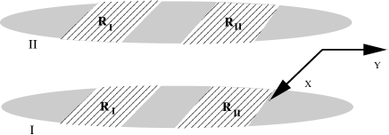
Figure 1: The experimental set-up corresponding to the Scheme I of our approach. The integration in $X$-direction is performed automatically by the imagine beam, whereas the integration in the $Y$-direction is done by ”hands”. The interference signal is collected from two disjoint regions $R_{I}$ and $R_{II}$.

Here we suggest two different setups to fix the problem with the unknown phase in Eq. (9). In the first setup, which we refer to as Scheme I (see Fig. (1)), we get rid of the random phase by making a special choice of the spatially separated integration domains. Namely instead of integrating $A^{2}$ over the entire region one splits the imaging area spanned by ${\bf r_{1}}$ and ${\bf r}_{2}$ to two spatially separated domains $R_{I}$ and $R_{II}$. In each experimental run one independently determines $A^{2}$ in the two domains then takes the absolute value of their square and averages over many experimental runs. As we will show in detail this setup relies on the fact that single particle correlation functions decay sufficiently fast with the distance, while the pair correlation functions decay slowly or do not decay at all. This setup has an obvious advantage compared to measuring $|A^{2}|^{2}$ because single particle normal correlation functions decay fast with the distance. As a result the quantity $A^{2}(\Omega_{1})A^{\star\,2}(\Omega_{2})$ is dominated by anomalous correlation functions:

$$\langle c_{\uparrow,I}^{\dagger}c_{\downarrow,I}^{\dagger}c_{\downarrow,II}c_{\uparrow,II}\rangle\approx\langle c_{\uparrow,I}^{\dagger}c_{\downarrow,I}^{\dagger}\rangle\langle c_{\downarrow,II}c_{\uparrow,II}\rangle,$$

where subscripts $I$ and $II$ indicate that spatially these operators are located in regions $R_{I}$ and $R_{II}$. Note that if the domains are not spatially separated or single particle correlations functions do not decay fast there are additional (unwanted) cross correlations in the equation above like $\langle c_{\uparrow,I}^{\dagger}c_{\uparrow,II}^{\dagger}\rangle\langle c_{\downarrow,I}^{\dagger}c_{\downarrow,II}\rangle$.

In the second setup, which we refer as Scheme II, (see Fig. (2)) we introduce a weak tunneling $t_{\perp}$ between the two layers. This tunneling locks the phases of pairing amplitudes in the two layers and makes the expectation value of $A^{2}$ real and positive. Besides the phase locking effect, the tunneling induces the mixing between the fermions in the two layers and results to the nonzero contribution to $A^{2}$ in Eq. (8) even in the absence of pairing. Below we will show that at small temperatures it is always possible to choose the tunneling such that phase locking transition already occurred but the correlation functions are not yet significantly affected so that Eq. (12) still holds.

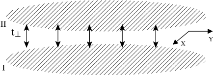
Figure 2: The experimental set-up corresponding to the Scheme II of our approach. The non-zero tunneling between two layers locks the phases of superfluids. The interference signal is collected now from the whole areas of superfluids.

The two setups are complimentary to each other and can be used depending on the situation. The Scheme I essentially relies on the existence of the long (or quasi-long) range order in the pairing amplitude. As we will show this scheme can be adopted to measuring not only the existence of superfluidity but also to the symmetry of the order parameter and even its phase. While the Scheme II is more sensitive to the local pairing between fermions and less to the existence of long range order in the superfluid phase. Such setup can be used, for example, to measure pseudo gap phenomena. Scheme II can also be used to determine the local symmetry of the pairing wave function but not its phase.

III Scheme I: Basic set-up and Various examples

Keeping the analogy with analysis of normal correlations we emphasize the integration region $R$ in the definition of the operator $A^{2}$ and denote it as $A^{2}(R)$ in what follows

$$A^{2}(R_{I})=A_{\uparrow}(R_{I})A_{\downarrow}(R_{I})=$$ (10)

$$= \int_{R_{I}}d{\bf r}_{1}\,\int_{R_{I}}d{\bf r}_{2}\,c^{\dagger}_{1\uparrow}({\bf r}_{1})c^{\dagger}_{1\downarrow}({\bf r}_{2})c_{2\downarrow}({\bf r}_{2})c_{2\uparrow}({\bf r}_{1})$$

Since for independent condensates the correlation function above factorizes into a product of anomalous correlation functions in each system and from Eq. (10) we arrive to Eq. (9). As we argued earlier, because $A^{2}(R_{I})$ is a complex number with a phase which is random from shot to shot, taking expectation value of equation (9) gives us zero. To get rid of this random phase we compare interference patterns from a pair of regions, $R_{I}$ and $R_{II}$. More precisely we take $[A^{2}(R_{I})]^{\dagger}A^{2}(R_{II})$, so that the random relative phase between pairing functions $F_{1}$ and $F_{2}$ drops out. Experimentally this procedure corresponds to taking a square of the Fourier transform of the density along $x$-direction integrated over the region $I$ and multiplying it by a complex conjugate of a similar quantity integrated over the region two. The result of this manipulation is then averaged over many experimental runs. Assuming that the system has a true long range order, taking regions $R_{I}$ and $R_{II}$ to be separated by a distance which is appreciably larger than the size of the Cooper pairs, and taking $R_{I}$ and $R_{II}$ to be identical we find

$$\langle[A^{2}(R_{I})]^{\dagger}A^{2}(R_{II})\rangle=$$

$$\left|\int_{R_{I}}d{\bf r}_{1}\,\int_{R_{I}}d{\bf r}_{2}\,F_{1}^{\star}({\bf r}_{1},{\bf r}_{2})F_{2}({\bf r}_{1},{\bf r}_{2})\right|^{2}$$ (11)

We now consider several specific examples in which analysis of expectation values of the type (11) can be used to identify interesting many-body states.

III.1 Analysis of the anomalous interference amplitude within the BCS theory

We now consider the integral in Eq. (11). To simplify calculations we also assume the translational invariance in both systems. In this case the pairing wave function depends only in the difference between ${\bf r}_{1}$ and ${\bf r}_{2}$: $F_{\alpha}({\bf r}_{1},{\bf r}_{2})\equiv F_{\alpha}({\bf r}_{1}-{\bf r}_{2})$. Then

$$A_{2}=2\mathcal{A}\int_{R}d{\bf r}F_{1}^{\dagger}({\bf r})F_{2}({\bf r}),$$ (12)

where the integration is again taken over the part of a condensate $R_{I}$ or $R_{II}$ with the imaging area $\mathcal{A}$. As we noted once the relative phase is taken care of and assuming the two condensates are identical we have $F_{1}=F_{2}$ and thus

$$A_{2}=2\mathcal{A}\int{d{\bf k}\over(2\pi)^{2}}|F({\bf k})|^{2},$$ (13)

The integral above can be easily evaluated within the BCS model (we take zero temperature limit)

$$A_{2}={\mathcal{A}\over 2}\int{d{\bf k}\over(2\pi)^{2}}{\Delta^{2}_{\bf k}\over E_{\bf k}^{2}}.$$ (14)

where the pairing function $\Delta_{\bf k}$ has to be specified for concrete type of pairing, $E_{\bf k}=\sqrt{\xi_{\bf k}^{2}+\Delta_{\bf k}^{2}}$ and $\xi_{\bf k}={\bf k}^{2}/2m-\mu$ is a single-particle dispersion. Thus if the pairing gap is isotropic and energy independent $\Delta_{\bf k}\equiv\Delta_{0}$ then in 2D we find

$$A_{2}^{(s)}={\mathcal{A}\rho_{0}\Delta_{0}\over 2}\arctan{\Delta_{0}\over\mu}.$$ (15)

where the 2D constant density of states $\rho_{0}$ is introduced. In the weak coupling limit $\Delta_{0}\ll\mu$, where $\mu$ is a chemical potential, we have $A_{2}\approx N{\Delta^{2}_{0}/4\mu^{2}}$, where $N\approx 2\mu\rho_{0}$ is the total number of particles (the factor of two takes into account two different spin components). If the pairing is strong then BCS extrapolation gives $A_{2}\approx N\pi/4$. We see that $A_{2}$ is a monotonically increasing function of the pairing gap and thus can serve as a direct probe of the fermionic superfluidity. Note that Eq. (14) can be also analyzed in the case of d-wave pairing, where $\Delta({\bf k})\sim\Delta_{0}\cos(2\theta_{\bf k})$, where $\theta_{\bf k}$ is the polar angle of the wave vector ${\bf k}$. The result is (see Appendix C)

$$A_{2}^{(d)}={\mathcal{A}\rho_{0}\over 2}2\pi\mu\left(\sqrt{1+\left(\frac{\Delta_{0}}{\mu}\right)^{2}}-1\right).$$ (16)

However, since only the square of $\Delta_{\bf k}$ enters Eq. (14) and we are explicitly averaging over angles, the difference between $s-$ and $d-$ parings will be minor. In fact one can show that in the $d-$wave case Eq. (15) gets multiplied by a smooth function of $\Delta_{0}/\mu$ which changes between $1/2$ at $\Delta_{0}\ll\mu$ and $2/\pi$ in the opposite limit.

III.2 Phase sensitive detection of the d-wave pairing

In the section above we discussed a possibility to detect anisotropy of the pairing amplitude using one-dimensional integration. In particular for the d-wave paring (dSF) the interference signal should vanish along the nodal directions. There are also other earlier suggestions for the detection of dSF, which rely rely on the detection of the Dirac like dispersion of quasiaprticles altman ; georges ; giamarchi_kohl ; HCZDL . This however is not a unique signature of the d-wave pairing state. A Dirac cone of quasi-particles may also arise for an anisotropic s-wave pairing scalapino or d-density wave states chakravarty .

Here we would like to show how the Scheme I can be extended to do phase sensitive detection of dSF. In high temperature cuprate superconductors, the crucial experiments which identified the $d$-wave character of pairing were phase sensitive experiments by Van Harlingen et al. vanHarlingen and Tsuei and Kirtley TK . These experiments unambiguously demonstrated the correct angular dependence of the pairing amplitude. Experimental set-up by Van Harlingen et al. used a combination of an s-wave and d-wave superconductors in a corner SQUID geometry. Interference of s-wave Cooper pairs with different parts of d-wave Cooper pairs was used to establish the relative phase of of the Cooper pair wave function.

What we discuss below is the cold atoms analogue of the Van Harlingen experiments. Hence we also need a source of s-wave Cooper pairs and a source of d-wave Cooper pairs. We imagine a pair of two dimensional fermionic systems, made of the same species of atoms, but having s-wave pairing in one layer and d-wave pairing in the other layer. This may be achieved, for example, using magnetic field dependence of the scattering length and applying a strong field gradient. Now we analyze interference patterns from two regions, $R_{I}$ and $R_{II}$, which differ only by the 90^o rotation. The quantity $A_{Q}(R_{I})$ is a complex number which has a random phase from one shot to another. Analogously $A_{Q}(R_{II})$ is a complex number with a random phase. But the $d$-wave symmetry of the pairing requires that phases of these two complex amplitudes differ by precisely $\pi$. Hence one can look at $\langle[A_{Q}(R_{I})]^{\dagger}A_{Q}(R_{II})\rangle$ and the d-wave symmetry dictates that this expectation value should be negative. On the other hand, when $R_{I}$ and $R_{II}$ have the same orientation, expectation value of $\langle[A_{Q}(R_{I})]^{\dagger}A_{Q}(R_{II})\rangle$ should be a positive number. It is important to emphasize that this statement is general and does not rely on the specific microscopic model for $d$-wave pairing. We stress that that only one of the layers should have a d-wave symmetry otherwise $A_{Q}$, being proportional to the product of anomalous correlation functions in two layers, does not change sign under rotations (see Eq. (12)). While the precise value of $\langle[A_{Q}(R_{I})]^{\dagger}A_{Q}(R_{II})\rangle$ is not easy to calculate, especially if we are dealing with non-identical superfluids, that statement of the $\pi$ phase difference between $A_{Q}(R_{I})$ and $B_{2}(R_{II})$ relies only on the $d$-wave nature of pairing.

The crucial feature of the method discussed in this subsection is that it should provide a qualitative and model independent signatures of d-wave pairing. It does not rely on detailed analysis of the microscopic models but it uses only the fundamental symmetry of the d-wave order parameter.

III.3 Probing of the anisotropy of pairing amplitude

We now discuss another probe of d-wave pairing. Unlike the previous method, it can not be used to demonstrate the change of the sign of the gap function $\Delta(k)$. However it can be used to observe anisotropy of the gap. We study the correlation function (8) but integrate it in a highly anisotropic way. In particular, one length, say along the probing beam should be macroscopic and the other $W$ should be shorter than the coherence length. Then (the square of) the anomalous interference amplitude becomes

$$a_{2}(\theta)=2\mathcal{A}W\int dz|F({z,\theta})|^{2},$$ (17)

where $\theta$ is the polar angle which defines direction of integration. We introduced a new notation $a_{2}$ to avoid possible confusion with $A_{2}$ analyzed earlier. Note that typically d-wave symmetry of the order parameter requires the presence of the optical lattice. This lattice in turn breaks rotational symmetry in the superfluid and locks the phase of the pairing amplitude with the lattice’s principal axes. Therefore there is no ambiguity in defining $\theta$ from one experimental run to another. One can expect that for $s-$ wave pairing (17) should give isotropic result, while for the $d-$ wave pairing the outcome will be highly anisotropic. While this approach does not provide a ”smoking gun” signature of the change of sign in the Cooper pair wavefunction, this method is easier to do experimentally; if successful it should provide a strong indication of anisotropic pairing.

It is straightforward to show that in the $s-$wave case the function $F$ is isotropic and is given by

$$F(z,\theta)=\rho_{0}\Delta\,J_{0}(z/\zeta)K_{0}(z/\xi),$$ (18)

where

$$\zeta^{2}={1\over\sqrt{k_{\mu}^{4}+k_{\Delta}^{4}}+k_{\mu}^{2}},\quad\xi^{2}={1\over\sqrt{k_{\mu}^{4}+k_{\Delta}^{4}}-k_{\mu}^{2}},$$

$k_{\mu}=\sqrt{2m\mu/\hbar^{2}}$ and $k_{\Delta}=\sqrt{2m\Delta/\hbar^{2}}$. This expression shows that the pairing wavefunction diverges logarithmically at small $z$ and decays exponentially with the characteristic correlation length $\xi$ at large $z$. The logarithmic divergence is the usual artifact of the BCS theory with point-like interactions. This divergence is cutoff at short distances.

Using Eqs. (18) we evaluate the integral in Eq. (16) and find

$$a_{2}=\frac{\pi^{2}}{2}\mathcal{A}W\rho_{0}^{2}\Delta^{2}\xi$$

$$~{}~{}~{}~{}~{}~{}~{}\times\!\!\!{\phantom{x}}_{4}F_{3}\left[\left({1\over 2},{1\over 2},{1\over 2},{1\over 2}\right),(1,1,1),-{\xi^{2}\over\zeta^{2}}\right],$$ (19)

where ${}_{4}F_{3}$ is the generalized Hypergeometric function. At small and large ratio of $\Delta/\mu$ the expression above gives the following asymptotics:

$$a_{2} \approx {\sqrt{2}\over 3\pi}\mathcal{A}W{\rho_{0}^{2}\Delta^{2}\over k_{\mu}}\ln^{3}\left(\Delta\over\mu\right),\quad\Delta\ll\mu;$$ (20)

$$a_{2} \approx \frac{18.8}{4}\,\mathcal{A}W{\rho_{0}^{2}\Delta^{2}\over k_{\Delta}},\qquad\Delta\gg\mu.$$ (21)

As before the high energy estimate of the asymptotics is the extrapolation of the BCS result to the strong coupling limit. For $d-$ wave pairing the correlation function $F(z_{\theta},0)$ vanishes along the nodal direction and thus $a_{Q}(\theta)$ should vanish as well. On the other hand, along the antinodal direction we can recover the asymptotics similar to $s-$ wave case,

$$a_{2}\approx\frac{1}{6\pi}\mathcal{A}W{\rho_{0}^{2}\Delta^{2}\over k_{\mu}}\ln^{3}\left(\frac{\Delta}{8\sqrt{2}\mu})\right),\quad\Delta\ll\mu.$$ (22)

For details of computations see Appendices B and C.

III.4 FFLO phase

One of the most intriguing suggestions for the paired states of fermions with attractive interactions is the idea of FFLO phase for systems with spin imbalance. This state corresponds to Cooper pairing at a finite momentum and has been a subject of extensive theoretical studies during the last couple of yearscombescot ; yip ; radzihovsky ; huse ; drummond ; others . Experimental situation remains unclear (for recent review see Ref. [KZ, ]). We now discuss how interference experiments can be adopted to look for the FFLO state. An earlier proposal for the detection of the FFLO phase can be found in Ref. [kunyang, ].

The FFLO phase is characterized by the finite center of mass momentum of the Cooper pairs so that $F({\bf r}_{1},{\bf r}_{2})=\langle c_{\uparrow}({\bf r}_{1})c_{\downarrow}({\bf r}_{2})\rangle\propto e^{\pm i{\bf Q}({\bf r}_{1}+{\bf r}_{2})/2}$. Therefore when one analyzes the anomalous interference amplitude one expects additional modulations which can be detected by taking an appropriate Fourier transform. This can be achieved by changing the integration procedure in Eqs. (4) and (12). We note that this integration is not equivalent for the two directions. In the direction of the $x$ axis, integration is done automatically by the laser beam. In the other direction, i.e. along the $y$ axis, it is performed “manually” by integrating interference fringes (see Fig. 2). An alternative approach is to take a Fourier transform of the interference amplitude $A_{\sigma}(y)=\int dxA_{\sigma}(x,y)$ along the $y$ axis. This can also be thought of as modifying the integral in equation (4)

$$A_{Q,\sigma}(R)=\int_{R}A_{\sigma}({\bf r})e^{iQ_{x}x}d{\bf r}=\int_{R}d{\bf r}e^{iQy}c^{\dagger}_{1\sigma}({\bf r})c_{2\sigma}({\bf r})$$

(23)

where we implicitly assume that the direction of the vector ${\bf Q}$ coincides with the direction of integration $x$, ${\bf Q}=(Q,0)$. Defining now

$$A_{2}(R)=\langle A_{Q,\sigma}(R)A_{Q,\sigma^{\prime}}(R)\rangle=$$ (24)

$$= \int_{R}d{\bf r}_{1}\int_{R}d{\bf r}_{2}e^{iQ(y_{1}+y_{2})}F_{1}^{\star}(r_{1},r_{2})F_{2}(r_{1},r_{2}).$$

In the FFLO phase $A_{2}$ should have additional peaks at $Q$ matching the finite momentum of the Cooper pair. The global unknown relative phase can be removed again either by multiplying the signal coming from two spatially separated imaging areas $R_{I}$ and $R_{II}$ or by introducing weak tunneling coupling between the layers as discussed in the next section.

One may be concerned that in rotationally invariant systems the direction of the FFLO ordering wavevectors will not generically coincide with the $x$ axis used for the observation. This issue should be avoided by using systems that do not have a rotational symmetry in the $xy$ plane. In fact, one of the most promising systems for observing the FFLO phase is an array of weakly coupled 1d systems huse ; drummond . In this case the ordering wave vector should be in the direction of the tubes.

IV Scheme II: Anomalous Correlation Functions in phase locked systems

Another way to overcome the effect of unknown relative phase detecting anomalous interference amplitude is to introduce a weak tunneling between the two layers (see Fig. 2). As it was shown in Refs. [mathey, ; giamarchi, ] such tunneling leads to the phase-locking transition. At the same time if the tunneling is sufficiently weak then correlation functions do not appreciably change and Eq. (12) is still valid. Below we will show that there is indeed a wide range of parameters where the phases between pairing amplitudes in two layers are locked and Eq. (12) gives the dominant contribution into the expression (8).

In the next section we analyze the effect of weak coupling more carefully. We will explicitly analyze only the case of two coupled $s$-wave super fluids. However, our results should be very general because precise nature of the symmetry of the pairing amplitude ($s$-wave, $d$-wave, FFLO, etc.) is not very important for the phase-locking phenomena.

IV.1 Role of the inter-layer coupling

Two imaging areas used in the set-ups discussed previously were needed to cancel the unknown relative phase between the order parameters in two layers. The same effect, however, can be achieved by introducing a weak tunneling coupling between the layers. Then phases of order parameters should lock mathey ; giamarchi and one does not have to combine signals from two different areas. Conversely different imaging areas can be used as independent sources so that one can effectively average $A_{2}$ over several independent imaging areas in a single experimental run.

As before we will work in the BCS limit. The BCS Hamiltonian of two coupled condensates reads

$$\mathcal{H}=\sum_{\bf k,\,\alpha}\psi_{\alpha}^{\dagger}({\bf k})\left(\varepsilon_{\bf k}\tau_{z}+\Delta_{\bf k}\tau_{x}\right)\psi_{\alpha}({\bf k})$$

$$-t_{\perp}\sum_{\bf k}(\psi_{1}^{\dagger}({\bf k})\tau_{z}\psi_{2}({\bf k})+\psi_{2}^{\dagger}({\bf k})\tau_{z}\psi_{1}({\bf k})),$$ (25)

where we used Nambu notations: $\psi_{\alpha,\uparrow}=c_{\alpha,\uparrow}$, $\psi_{\alpha,\downarrow}=c_{\alpha,\downarrow}^{\dagger}$, $\alpha=1,2$ corresponds to two different layers, and $\tau_{x}$ and $\tau_{z}$ are the Pauli matrices. It is convenient to introduce symmetric and antisymmetric combinations: $\psi_{+}=(\psi_{1}+\psi_{2})/\sqrt{2}$ and $\psi_{-}=(\psi_{1}-\psi_{2})/\sqrt{2}$. The the Hamiltonian splits into the symmetric and antisymmetric parts $\mathcal{H}=\mathcal{H}_{+}+\mathcal{H}_{-}$:

$$\mathcal{H}_{\pm}=\sum_{\bf k}\psi_{\pm}^{\dagger}({\bf k})\left[(\varepsilon_{\bf k}\pm t_{\perp})\tau_{z}+\Delta_{\bf k}\tau_{x}\right]\psi_{\pm}({\bf k}).$$ (26)

Let us now find the effect of $t_{\perp}$ on $A_{2}$ using Eq. (8). Reexpressing the operators $c_{\alpha}$ and $c^{\dagger}_{\alpha}$ through the Nambu spinors $\psi$ and $\psi^{\dagger}$ and using Wick’s theorem and expanding to the leading order in the tunneling coupling $t_{\perp}$ it is straightforward to show that

$$A_{2}=A_{2,1}+A_{2,2}+A_{2,3},$$ (27)

where

$$A_{2,1}\approx{\mathcal{A}\over 2}\int{d{\bf k}\over(2\pi)^{d}}{\Delta_{\bf k}^{2}\over E_{\bf k}^{2}}$$ (28)

$$A_{2,2}\approx{\mathcal{A}^{2}t_{\perp}^{2}\over 4}\left[\int{d{\bf k}\over(2\pi)^{d}}{\Delta_{\bf k}^{2}\over E_{\bf k}^{3}}\right]^{2},$$ (29)

$$A_{2,3}\approx 2\mathcal{A}t_{\perp}^{2}\int{d{\bf k}\over(2\pi)^{d}}{\Delta_{\bf k}^{4}\over E_{\bf k}^{6}}.$$ (30)

Here $E_{\bf k}^{\pm}=\sqrt{(\varepsilon_{\bf k}\pm t_{\perp})^{2}+\Delta_{\bf k}^{2}}$.

Note that $A_{2,1}$ coincides with our earlier expression (14). The two other terms $A_{2,2}$ and $A_{2,3}$ are proportional to $t_{\perp}^{2}$. We point that $A_{2,2}$ scales faster with the imaging area than the other terms. The reason is that even in the absence of superfluidity the tunneling forces fermions to occupy preferably the symmetric state. This is in turn equivalent to establishing a well defined relative phase between the two atomic systems. Since we are interested in detecting $A_{2,1}$ and not $A_{2,2}$ in fermionic systems, contrary to bosonic, it is preferable to make the imaging area as small as possible, of the order of the Cooper pair size (or superconducting coherence length). Indeed the integral in Eq. (12) converges at long distances thus there is no need to go to ${\bf r}$ larger than the coherence length. The third term $A_{2,3}$ comes from the Andreev process. It is always subdominant at small $t_{\perp}$ and we can safely ignore it.

For the $s-$ wave pairing the integrals above can be explicitly evaluated:

$$A_{2,1}\approx{\mathcal{A}\rho_{0}\Delta\over 2}\arctan{\Delta\over\mu},$$ (31)

$$A_{2,2}\approx\left[{\mathcal{A}t_{\perp}\rho_{0}\over 2}\left(1+{\mu\over\sqrt{\mu^{2}+\Delta^{2}}}\right)\right]^{2}.$$ (32)

In the weak and strong pairing regimes we have the following asymptotics:

$$A_{1,2} \approx {\mathcal{A}\rho_{0}\Delta^{2}\over 2\mu^{2}},\;A_{2}^{2}\approx\mathcal{A}^{2}\rho_{0}^{2}t_{\perp}^{2},\quad{\rm\Delta\ll\mu}$$ (33)

$$A_{1,2} \approx {\pi\over 4}\mathcal{A}\rho_{0}\Delta,\;A_{2}^{2}\approx{1\over 2}A^{2}t_{\perp}^{2}\rho_{0}^{2},\quad{\rm\Delta\gg\mu}.$$ (34)

Both at weak and strong pairing we find that

$${A_{2,2}\over A_{2,1}}\sim\sqrt{n\mathcal{A}}\,{t_{\perp}\over\Delta},$$ (35)

where $n$ is the atom density. The $A_{2,2}$ contribution is an unwanted correction coming from the interlayer coupling, which have nothing to do with superfluidity. This contribution can be suppressed either by decreasing the tunneling amplitude $t_{\perp}$ or by decreasing the imaging area $\mathcal{A}$. Note that the tunneling amplitude can not be pushed down all the way to zero, because then one will loose phase coherence between the two layers. In the next section we will see that it is always possible to find the regime where $A_{2,2}$ is negligible and at the same time the two superfluids are locked. We also comment that one can distinguish two contributions $A_{2,1}$ and $A_{2,2}$ by looking into the dependence of $A_{2}$ on $t_{\perp}$.

IV.2 Phase locking transition

In this section we examine the effect of the tunneling coupling on establishing phase coherence between the two fermionic superfluids. From a prior work it is known that tow energy phase fluctuations in superfluids can be described by means of a conventional $xy$ model with the effective Lagrangian simanek ; thouless ; stone :

$$\mathcal{L}=n\dot{\theta}-{n\over 4m}(\nabla\theta)^{2}-{1\over 16mn}(\nabla n)^{2}-{(n-n_{0})^{2}\over 2\rho_{0}},$$ (36)

where

$$n=n_{0}-\rho_{0}(\dot{\theta}+(\nabla\theta^{2})/4m)$$ (37)

plays the role of the superfluid density, $\theta$ is the phase of the superfluid order parameter. We emphasize that if fluctuations of $\theta$ are small then $n$ is close to the total density of atoms. It is straightforward to generalize the derivation of the Lagrangian given in Ref. [thouless, ] to the bilayer system. A similar derivation but for a tunneling through a point can be also found in Ref. [simanek, ] and it is sketched in Appendix B for completeness. We use this formalism to evaluate the tunneling Hamiltonian from the effective action given in Eq. (71).

In the case of $s-$ and $d$-wave pairings the integral appearing in Eq. (71) can be easily evaluated yielding the following coupling term to the Hamiltonian of the system:

$$\mathcal{H}_{12}=-\frac{t_{\perp}^{2}}{8\pi}\rho_{0}T(\Delta/\mu)\cos(\theta_{1}-\theta_{2}).$$ (38)

where the functions $T(\Delta/\mu)$ for the $s-$ and $d-$ wave pairings are given in Appendix C. In both cases $T(\Delta/\mu)$ is a smooth function, which interpolates between $T(\Delta/\mu)\approx 2$ at $\Delta\ll\mu$ and $T(\Delta/\mu)\approx 1$ in the opposite limit. When the pairing is small $\Delta\ll\mu$ the effective Josephson coupling becomes simply $J\approx t_{\perp}^{2}\rho_{0}$, i.e. independent on $\Delta$. This is a bit surprising result since one would naively expect that $J$ should vanish as $\Delta\to 0$. And this is indeed the case in superfluids with inhomogeneous tunneling where $J\sim t_{\perp}^{2}\rho_{0}^{2}\Delta$ (see Ref. [simanek, ] for details). In superfluids with uniform $t_{\perp}$ the Josephson coupling gets enhanced by the coherence factor $1/(\rho_{0}\Delta)\sim k_{f}\xi$, where $\xi$ is the BCS coherence length, and the dependence of $J$ on $\Delta$ disappears.

The minimal tunneling required to lock the two phases together between two superfluids can be estimated from equating the energy gap required to transfer one particle from one superfluid to another

$$E_{c}\approx{1\over\rho_{0}L^{2}}$$ (39)

to the energy gain due to the tunneling term

$$E_{J}\approx t_{\perp}^{2}\rho_{0}L^{2},$$ (40)

where $L^{2}$ is the area of each condensate. Note that $L^{2}$ can be significantly larger than the imaging area $\mathcal{A}$. From these equations we find that $E_{J}>E_{c}$ is equivalent to

$$t_{\perp}>{1\over\rho_{0}L^{2}}.$$ (41)

This condition is compatible with the dominance of $A_{1}$ over $A_{2}$ in Eq. (35) if

$$\Delta>{1\over\rho_{0}L^{2}}\sqrt{n\mathcal{A}}.$$ (42)

In the weak coupling limit $\Delta\ll\mu$ this requirement reduces to $\Delta>\mu\sqrt{\mathcal{A}/nL^{4}}$ and in the strong coupling regime $\Delta\geq\mu$ Eq. (42) reduces to $\sqrt{\mathcal{A}/nL^{4}}\ll 1$. Clearly both conditions can be easily satisfied using either small imaging areas or systems with sufficiently large number of particles $nL^{2}$.

For convenience we assumed the zero temperature case throughout the paper. However, we would like to stress that our results will be robust to the effects of temperature as long as it is below the temperature corresponding to the Kosterlitz-Thouless transition. Indeed in coupled condensates it is the global phase which is destroyed by thermal fluctuations, but the relative phase remains locked all the way to the Kosterlitz-Thouless transition mathey .

IV.3 Discussion

Having the effective action for the fluctuations of the order parameter phase we can lift the assumption used in derivation of Eq. (32) that the phases between two superfluids are locked together and get

$$A_{2,1}\approx{\mathcal{A}\rho_{0}\Delta\over 2}\arctan{\Delta\over\mu}\mathrm{e}^{-\langle\theta^{2}\rangle/2}\approx{\mathcal{A}\rho_{0}\Delta\over 2}\arctan{\Delta\over\mu}$$

$$~{}~{}~{}~{}~{}~{}\times\exp\left(-{1\over 2\rho_{0}t_{\perp}T_{S,D}(\Delta/\mu)L^{2}}\right).$$ (43)

We note that $A_{2,2}$ is not sensitive to the relative phase between the two superfluids and thus Eq. (32) holds for an arbitrarily small $t_{\perp}$.

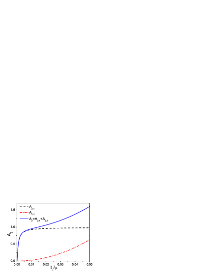
Figure 3: Anomalous interference amplitude $A_{2}=A_{2,1}+A_{2,2}$ and separately contributions $A_{2,1}$ (Eq. (43)) and $A_{2,2}$ (Eq. (32)) versus tunneling $t_{\perp}/\mu$ for sample parameters (see text for details). The red line ($A_{2,2}$) is the contribution, which comes from normal fermions, the black line is the superfluid contribution.

In Fig. 3 we plot $A_{2}=A_{2,1}+A_{2,2}$ and separately contributions $A_{2,1}$ (Eq. (43)) and $A_{2,2}$ (Eq. (32)) versus tunneling $t_{\perp}/\mu$ for sample parameters $\Delta/\mu=0.2$, $\mathcal{A}/L^{2}=0.02$, $N=10^{3}$, where $N$ is the total number of fermions per condensate. The graph indicates that there is an intermediate tunneling regime, where the superfluid contribution $A_{2,1}$ dominates over the normal part $A_{2,2}$. We note that because $A_{2,2}$ is not sensitive to the superfluid gap one can perform separate measurements of $A_{2}$ in the normal and superfluid regimes. Then the difference between the two will be precisely given by $A_{2,1}$.

So far considering interlayer coupling we focused only on large imaging areas, with both transverse and longitudinal dimensions large compared to microscopic length scales. In the opposite limit one has to study the correction to Eq. (12). Instead of repeating rather tedious analysis of Sec. IV.1 we will make a couple of simple points. (i) There will be additional contribution to $a_{2,2}(\theta)$ which scales as $t_{\perp}^{2}$. This contribution will have the same origin as $A_{2,2}$ in Eq. (32) and will be insensitive to superfluidity. (ii) This unwanted contribution will be greatly suppressed because it scales as the square of the imaging area, which is small since one length scale is microscopic. Thus the effect of the inter-layer coupling on the interference in this case will be even smaller than in the case of the macroscopic imaging area.

V Anomalous correlation functions in Bose systems

So far the main focus of our work was analysis of the possibility of measuring anomalous correlation functions in fermionic superfluids. There such measurements are key for determination of the pairing gap. On the contrary one can get substantial information about the superfluid properties of Bose systems analyzing normal correlation functions paris ; PAD ; GADP . Nevertheless the possibility to measure anomalous correlation functions can provide additional valuable information about properties of these systems. As we will see below these functions have very unusual behavior in the systems with quasi-long order like zero-temperature one-dimensional and finite-temperature two-dimensional systems. In this section we will give explicit results both for 1D and 2D systems.

We consider setup analogous to that discussed in Sec. IV. Using the same arguments we find that

$$A_{2}=\mathcal{A}\int_{{\bf r}\in\mathcal{A}}d^{d}rF_{1}^{\star}({\bf r})F_{2}({\bf r}),$$ (44)

where $F_{\alpha}({\bf r})=\langle a_{\alpha}({\bf r})a_{\alpha}(0))$, $\alpha=1,2$; $\mathcal{A}$ is the imaging area for $2D$ systems and the imaging length in the $1D$ setup. The operators $a_{\alpha}$ have bosonic statistics. As in the case with fermions $A_{2}$ vanishes if the two systems are uncoupled. However, as we argue below if the imaging area is smaller than the system size, one can always find the regime of small transverse tunnelings $t_{\perp}$ such that the phases of two superfluids are locked together, but the correlation functions remain independent of $t_{\perp}$. In this case assuming that the two systems are identical, as in Sec. IV, we have

$$A_{2}\approx\mathcal{A}\int_{{\bf r}\in\mathcal{A}}d^{d}r|F({\bf r})|^{2},$$ (45)

where $F$ describes anomalous correlation functions in either of the two systems. We note that the scheme I, where we use two imaging areas can not be straightforwardly applied to bosons because the single particle correlation functions decay slowly. However, in bosonic systems one can deal even without tunneling for the following reason. The relative phase between two independent superfluids is random from shot to shot. Nevertheless in each shot the interference amplitude is well defined and fluctuates only weakly PAD ; paris . Thus this unknown relative phase can be reliably determined in each run. Then one can evaluate anomalous correlation functions putting the origin of integration along $z$ in the position of the central interference peak. It is easy to see that this procedure eliminates the effect of the unknown phase and leads to Eq. (45).

V.1 One-dimensional superfluids

Let us first analyze Eq. (45) for two coupled Bose systems at zero temperature. If the imaging length is larger than the healing length of the condensate then boson-boson correlation functions are approximately

$$\langle a(x)a(0)\rangle\propto\left(\frac{x}{L}\right)^{1\over 2K}+\ldots,$$ (46)

where $K$ is the Luttinger parameter related to the interaction strength (see e.g. Ref. [caz, ]) and $L$ is the length of a system. Dots indicate other contributions which scales with larger power and thus their contribution is less important. For a Lieb-Liniger gas with short range repulsive interactions $K\gg 1$ in the weakly interacting Gross-Pitaevskii regime and $K\to 1$ in the fermionized Tonks-Girardeau regime. Notice that this correlation function increases with the distance. This unusual behavior also reflects the scaling of $B_{Q}^{2}$ with the imaging length $\mathcal{A}$:

$$A_{2}(\mathcal{A})\sim\tilde{C}\mathcal{A}^{2}\left(\mathcal{A}\kappa\right)^{1\over K},\;\mathcal{A}\kappa\ll 1$$

$$A_{2}(\mathcal{A})\sim\tilde{C}\mathcal{A}^{2},\quad\mathcal{A}\kappa\gg 1,$$ (47)

where $\tilde{C}$ is a nonuniversal constant and $\kappa\propto\sqrt{t_{\perp}}$ is the characteristic wavevector corresponding to the transverse tunneling (see details below). At sufficiently short distances the anomalous interference amplitude $A_{2}$ grows faster than the area squared. As the imaging size approaches the cutoff length the superlinear dependence becomes linear and we recover the expected result for the system with a long-range order.

We can make the analysis more quantitative using low-energy description of two coupled one-dimensional Bose systems (see e.g. Ref. [gpd, ] for more details). In particular, for weakly interacting superfluids it can be shown that the Lagrangian governing properties of the relative phase $\phi(x,\tau)$ between the condensates is:

$$\mathcal{L}(x,\tau)={v_{s}K\over 4\pi}\left[{1\over v_{s}^{2}}(\partial_{\tau}\phi)^{2}+(\partial_{x}\phi)^{2}-2\kappa^{2}\cos(\phi)\right],$$ (48)

where $\tau$ is the imaginary time, $v_{s}$ is the sound velocity in each condensate, and $\kappa^{2}\approx 4\pi t_{\perp}n/v_{s}K$.

The analysis of either normal or anomalous correlation functions can be performed using the form-factor approach. For more details on this approach we refer to Ref. [EK, ] for a general scheme and to Ref. [gpd, ] for the application to the one-dimensional condensates. This analysis is rather involved for generic value of the interaction parameter $K$ and requires summation of many contributions coming from the intermediate processes including creation and annihilation of soliton-antisoliton pairs as well as their bound states- breathers. Anomalous correlation functions would correspond in that case to the soliton-creating or soliton-annihilating form-factors LZ . On the other hand for weak interactions (large $K$) the Lagrangian can be simplified even further if we invoke Gaussian approximation replacing $\cos(\phi)$ by $1-\phi^{2}/2$. More carefully, this can be done using the self-consistent harmonic approximation gia . In this simple Gaussian approximation the calculation of anomalous correlation function becomes trivial and we get

$$F(x)=\langle a_{1}^{\dagger}(x)a_{2}(x)a_{1}^{\dagger}(0)a_{2}(0)\rangle\approx C\langle\mathrm{e}^{i(\phi(x)+\phi(0))}\rangle$$

$$=C^{\prime}\left({\kappa\over\Lambda}\right)^{1\over K}\!\exp\left(-{2\pi\over K}{1\over\kappa L}\right)\exp\left[-{1\over K}K_{0}(\kappa x)\right]\!,$$ (49)

where $C$ and $C^{\prime}$ are nonuniversal numerical factors and $\Lambda$ is the short-distance cutoff of the order of inter-particle density $\Lambda\sim n$ (we assume that $\kappa/\Lambda\ll 1$). The first exponential factor appearing in the equation above is similar to that, which we discussed earlier (see Eq. (43)). It shows that for small enough $t_{\perp}$ such that $\kappa\lesssim 2\pi/KL$ the phases between two superfluids are not locked and anomalous correlations are exponentially suppressed. If on the other hand the opposite is true the phases are locked together and this term is close to unity. And finally the last multiplier gives the spatial dependence of the correlation function $F(x)$. At $\kappa x\ll 1$ we have $K_{0}(\kappa x)\approx-\ln(\kappa x)$ and we recover the asymptotic $F(x)\propto x^{2/K}$,in the opposite limit $\kappa x\gg 1$ we have $K_{0}(\kappa x)\ll 1$ and thus $F(x)\approx{\rm const}(x)$.

Using Eq. (49) we find that

$$A_{2}=\mathcal{A}C^{\prime\,2}\left({\kappa\over\Lambda}\right)^{2\over K}\exp\left[-{4\pi\over K}{1\over\kappa L}\right]$$

$$~{}~{}~{}~{}~{}~{}~{}\times\int\limits_{0}^{\mathcal{A}}dx\exp\left[-{2\over K}K_{0}(\kappa x)\right].$$ (50)

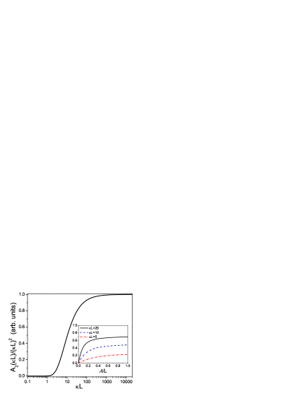
Figure 4: The ratio of $A_{2}$ and $(\kappa L)^{2}$ vs. $\kappa L$ for imaging length equal to the system size $\mathcal{A}=L$; $\kappa\propto\sqrt{t_{\perp}}$ is the characteristic wavevector related to the gap $\Delta$ (see Eq. 48). The inset shows $A_{2}/\mathcal{A}^{2}$ as a function of $\mathcal{A}/L$ for different values of $\kappa L$. The superlinear behavior of $A_{Q}$ vs. $\mathcal{A}$ is a consequence of unusual behavior of anomalous correlation function $F(x)\sim\langle\exp[i(\phi(x)+\phi(0))]$.

In Fig. 4 we plot the dependence of $A_{2}/(\kappa L)^{2}$ on $\kappa L$ for the imaging size equal to the system size $\mathcal{A}=L$. At small tunneling $\kappa L\ll 1$ the two condensates are decoupled and the anomalous correlator is exponentially suppressed. As the transverse tunneling increases $\kappa L\sim 1$ the anomalous interference amplitude increases faster than linearly and at $\kappa L\gg 1$ we have $A_{2}\propto L$. Note that there is a very wide range of parameters $3\lesssim\kappa L\lesssim 100$, where the superlinear behavior can be observed. Similarly one can fix the transverse tunneling and the system size and analyze the dependence of $A_{2}$ as a function of the imaging size. The inset shows such plots for different values of $\kappa L$. Again one observes the superlinear behavior of $A_{2}$ in a wide regime of parameters. We remind that the normal interference amplitude $A_{Q}$ defined in Sec. II.1 always has sublinear behavior PAD ; GADP ; IGD .

We can easily generalize the analysis above to the case of finite temperatures. In the regime when the thermal coherence length $\xi_{T}\approx Kv_{s}/T$ is large compared to the healing length of the condensates the phase model described the Lagrangian (48) gives the correct low energy description of the two coupled superfluids. Within this model one finds

$$\langle a(x)a(0)\rangle=n\exp\left[-{4\pi\over KL}\sum_{q}{\coth{v_{s}\sqrt{q^{2}+\kappa^{2}}\over 2T}\over\sqrt{q^{2}+\kappa^{2}}}\cos^{2}{qx\over 2}\right].$$ (51)

In the zero temperature limit this expression reduces to Eq. (49) while at $T\geq v_{s}\kappa$ we get

$$\langle a(x)a(0)\rangle\approx n\exp\left[-{\pi T\over K\kappa v_{s}}\left(1+\mathrm{e}^{-\kappa x}\right)\right].$$ (52)

In this case we have exponentially increasing correlations

$$\langle a(x)a(0)\rangle\sim\exp\left({\pi T(x-2/\kappa)\over Kv_{s}}\right)$$ (53)

for $\kappa x\leq 1$ and then their saturation as $\kappa x$ becomes larger than one. In turn this behavior of the correlation functions implies that in the regime $T\geq\kappa v_{s}$ the anomalous interference amplitude scales as

$$A_{2}\propto\mathcal{A}\exp\left({2\pi T\over Kv_{s}}\mathcal{(}A-2/\kappa)\right)$$ (54)

at $\mathcal{A}\ll 1/\kappa$ and then in the usual way $A_{2}\sim\mathcal{A}^{2}$ in the opposite limit. Thus anomalous correlation functions can be used to probe the temperature in the system. We note, however, that in the high temperature regime $T\gg\kappa v_{s}$ the anomalous interference amplitude $A_{Q}$ is exponentially suppressed.

V.2 Two-dimensional superfluids.

In a similar fashion to the previous section we can analyze behavior of the anomalous correlation functions and the anomalous interference amplitude for two-dimensional bosonic superfluids. Below the Kosterlits-Thouless phase transition temperature the low energy properties of the superfluids can be described by the effective Lagrangian (defined as the ratio of the energy density to the temperature), which is very similar to (48):

$$\mathcal{L}({\bf r})\approx{\hbar^{2}\rho_{s}\over 4mT}\left((\nabla\phi)^{2}-2\kappa^{2}\cos\phi\right),$$ (55)

where as before $\phi$ is the local phase difference between the two superfluids, $T$ is the temperature, $\rho_{s}$ is the superfluid density, $m$ is the boson’s mass, and $\kappa^{2}\approx 4mt_{\perp}/\hbar^{2}$. Because of the formal analogy of Lagrangians (55) and (48) the anomalous correlation function $F({\bf r})=\langle a({\bf r})a(0)\rangle$ in two dimensions is identical to Eq. (49) under the substitution $K\to\pi\hbar^{2}\rho_{s}/(mT)$ and $v_{s}\to 1$. So one can expect a similar superlinear behavior of the anomalous interference amplitude $A_{2}$:

$$A_{2}\sim\mathcal{A}^{2+1/2K}$$ (56)

for $\kappa\sqrt{\mathcal{A}}\ll 1$ and $A_{2}\sim\mathcal{A}^{2}$ in the opposite limit.

V.3 Paired multicomponent bosonic condensates

Condensates of atom pairs can also be realized with bosonic atoms. The original idea of fragmented condensates goes back to Nozieres and Saint Jamesnozieres . They emphasized the difficulty of achieving such states since attraction between bosonic atoms favors binding not just two but many particles and may lead to the system collapse. More recently, paired condensates were discussed by Kuklov et al. kuklov for a two component bosonic mixture in an optical lattice. Perhaps the most natural setting for the appearance of bosonic pairing is polar condensates of $S=1$ atoms in two dimensionsohmi ; ho ; zhou . As discussed in Refs. [mukerjee, ,podolsky, ], in such systems general topological considerations suggest the appearance of quasi-long range order for singlet pairs rather than individual spinor components. This is the system that we focus on in this subsection.

Let $\psi_{\alpha}(r)$ be individual spinor components with $m=\pm 1,0$. We can make a spin singlet pair operator $\Delta(r)=\psi_{+1}(r)\psi_{-1}(r)+\psi^{2}_{0}(r)$. As discussed in Refs. [mukerjee, ; podolsky, ] for two dimensional polar condensates, such as ${}^{23}Na$, one expects to find a phase in which $\langle\Delta^{\dagger}(r_{1})\Delta(r_{2})\rangle$ shows power law correlations. At the same time there are only short range correlations for individual spin components. In an interference experiment from a pair of independent $S=1$ polar condensates one should measure interference amplitude for individual spin components, $A_{m\,R}$, then construct $A_{R}=A_{+1\,R}A_{-1\,R}+A_{0R}$. In each shot the phase of $A(R)$ is random, so one can again take two regions, $R_{I}$ and $R_{II}$, and consider $\langle A_{R_{I}}^{\dagger}A_{R_{II}}\rangle$. This expectation value should decay as a power law of the distance between the two regions.

VI Summary and Conclusions

In this paper we addressed questions of application of interference experiments to detect paired states of either fermions or bosons in low dimensions. We showed that direct generalizations of approaches used in analyzing interference of independent bosonic condensates do not work due to overwhelming shot noise contribution. Thus we proposed and analyzed two alternative schemes of interference experiments which can be used to study anomalous correlation functions, which contain information about pairing amplitudes. These (gauge-noninvariant) correlation functions provide complimentary information to normal correlation functions and can be used to characterize the properties of the superfluids.

It was shown how the method of studying the anomalous functions can be used to detect various pairing orders. One of the scheme we propose is based on the phase sensitive detection employed earlier in the condensed matter systems. On the other hand, another scheme deals with two superfluids weakly coupled by interlayer tunneling. We establish the condition of validity of this scheme which involves the tunneling strength, imaging area and the system size. We emphasized important roles of different form of expansion (transversal and longitudinal) and directions of observation. In the case of bosonic superfluids anomalous correlation functions have an unusual property that they increase with the separation between quasiparticles.

VII Acknowledgements

We would like to thank E. Altman, A. Aspect, J. Dalibard, V. Galitski, M. Greiner, Z. Hadzibabic, M. Lukin, J. Schmiedmayer, and M. Zwierlein for discussions. A.P. acknowledges support from AFOSR YIP. V.G. and E. D. are supported by AFOSR, DARPA, MURI, NSF DMR-0705472, Harvard-MIT CUA.

Appendix A Expectation values of the normal correlations for the systems with pairing

In the BCS approximation the expectation value of the square of the interference fringe amplitude discussed in Sec. II can be found as

$$\langle|A|^{2}\rangle=\mathcal{A}\int{d{\bf k}\over(2\pi)^{d}}\left(1-{\xi_{\bf k}\over E_{\bf k}}\right)^{2},$$ (57)

where $n_{f}(E_{\bf k})$ is the Fermi distribution function, $E_{\bf k}=\sqrt{\xi_{\bf k}^{2}+\Delta_{\bf k}^{2}}$, $\xi_{\bf k}={\bf k}^{2}/2m-\mu$, $\mathcal{A}$ is the imaging area of the interference. The pairing gap function $\Delta_{k}$ is a constant $\Delta_{0}^{(s)}$ for the $s$-wave pairing and the $k$-dependent function $\Delta_{k}=\Delta_{0}^{(d)}(\cos(k_{x})-\cos(k_{y}))$ for the case of the $d$-wave pairing. In the absence of superconductivity and at zero temperature $|A|^{2}=2N$, where $N$ is the total number of fermions in each system. The nonzero value of $|A|^{2}$ in this case simply reflects anti-bunching of fermions (note the negative sign in Eq. (3)). As expected for fermions $A\sim\sqrt{N}$ (see e.g. Ref. [P, ]).

Considering $s$-wave pairing and using the constant density of states $\rho_{0}$ in $2D$ one finds

$$|A|^{2}=\!2N\!-\!\mathcal{A}\Delta_{0}^{(s)}\rho_{0}\left({\pi\over 2}+\arctan(t_{s})-2[t^{2}_{s}+1]^{\frac{1}{2}}\right)\!\!,$$

(58)

where $t_{s}=\mu/\Delta_{0}^{(s)}$ and $\mu$ is the chemical potential. In the BCS limit $\mu\gg\Delta_{0}^{(s)}$ the equation above reduces to $A_{2}\approx 2N-\mathcal{A}\pi\rho_{0}\Delta_{0}^{(s)}$. If we formally extrapolate $BCS$ theory towards the unitarity limit $\mu\to 0$ and $\Delta_{0}^{(s)}\to n/\rho_{0}$ then $A_{2}\to N(2-\pi/2)$. So we see that $A_{2}$ is a monotonically decreasing function of the pairing gap. The results will be somewhat different for the superfluids with the $d-$wave pairing in which case is

$$\langle|A|^{2}\rangle = 2N+2{\cal A}\rho_{0}\Delta_{0}^{(d)}([t^{2}_{d}+1]^{\frac{1}{2}}$$ (59)

$$+ 2t{\bf E}(-t^{-2}_{d})+2(1+t_{d}^{2})^{\frac{1}{2}}{\bf E}(\frac{1}{1+t_{d}^{2}}))$$ (60)

where $t_{d}=\mu/\Delta_{0}^{(d)}$.

Appendix B Transversal vs. Longitudinal expansions

In this Appendix we compare the two regimes of expansions: the transversal expansion advocated in the main text versus longitudinal one which is more close to to the standard time-of-flight technique.

The quantity similar to $A_{2}$ in Eq. (12) can be also measured in the standard time of flights experiments. For the low-dimensional superfluidity it is advantageous to have longitudinal expansion so that the atoms from different layers do not mix with each other. If one assumes that the interactions are not important during the expansion then the spatial image of the cloud after time of flight gives the momentum distribution of atoms in the initial condensate. As it is shown in Ref. [adl, ] the density-density correlation maps to the Fourier transform of the pairing amplitude:

$$\langle n({\bf R},t)n(-{\bf R},t)\rangle=|F({\bf Q})^{2}|,$$ (61)

where $Q=mR/\hbar t$. We note that the transverse expansion discussed in the previous section directly probes the spatial structure of (the square of) the pairing wave function and thus gives a complimentary information to the quantity (61). If one integrates Eq. (61) over the momentum ${\bf Q}$ then one recovers the expression identical to Eq. (13). So the two setups give equivalent information. We note, however, that in the transverse expansion regime one can benefit from independently averaging over several imaging areas within a single shot.

Doing the longitudinal expansion one can also determine the spatial structure of the pairing amplitude. Indeed if one integrates Eq. (61) along a preferred direction then the outcome should be isotropic for the $s-$ wave pairing and highly unisotropic in the $d-$ wave regime. Thus within the BCS model in the $s-$wave case and in the $d-$ wave case if one integrates along the anti-nodal direction (where the pairing gap is maximal) one gets

$$\int dx\langle n({\bf R},t)n(-{\bf R},t)\rangle\propto\Delta{\sqrt{\mu+\sqrt{\mu^{2}+\Delta^{2}}}\over\sqrt{\mu^{2}+\Delta^{2}}}.$$ (62)

On the other hand if one integrates Eq. (61) along the nodal direction in the $d-$ wave case (i.e. the direction where the pairing gap vanishes) one should get zero.

The clear advantage of the longitudinal expansion method is that one avoids the issues with coupling between different layers. In principle, one can perform this experiment even on a single layer. However, there is a big disadvantage too. Namely, one has to rely on the free expansion to get the right correlation functions. In the case of a bilayer system predominantly transverse expansion is guaranteed by the large kinetic energy of the transverse confinement. On the other hand for the longitudinal expansion collisions between atoms shortly after expansion started can affect the outcome of the experiment. We note that instead of purely longitudinal expansion one can have the full three-dimensional time of flight experiment and get similar results. However, if one is interested in two-dimensional superfluidity allowing expansion in all three dimensions one clearly looses in the signal to noise ratio.

Appendix C Effective action approach to coupled systems

The effective action ($S_{\rm eff}=\int_{0}^{\infty}\mathcal{L}(\tau)d\tau$) for the phase fluctuations reads thouless :

$$S_{\rm eff}[\theta_{1},\theta_{2}]={\rm Tr}\sum_{n=1}^{\infty}(\mathcal{G}_{0}\Sigma)^{n}$$

$$-{1\over 2g}\int d^{d}rd\tau\,(|\Delta_{1}({\bf r},\tau)|^{2}+|\Delta_{2}({\bf r},\tau)|^{2}),$$ (63)

where $g$ is the interaction strength, which we assume to be short range, $\mathcal{G}_{0}$ and $\Sigma$ are $4\times 4$ matrices:

$$\mathcal{G}_{0}=\left(\begin{array}[]{cc}G_{1}&0\\ 0&G_{2}\end{array}\right),\quad\Sigma=\left(\begin{array}[]{cc}\Sigma_{1}&T\\ T^{\dagger}&\Sigma_{2}\end{array}\right).$$ (64)

Here $G_{1,2}$ are the fermion’s Green’s functions in the superfluid with a non-fluctuating phase. In the Nambu notation their inverses are:

$$G_{1,2}^{-1}=\left(\begin{array}[]{cc}\partial_{\tau}-{\hbar^{2}\over 2m}\nabla^{2}&|\Delta_{1,2}|\\ |\Delta_{1,2}|&\partial_{\tau}+{\hbar^{2}\over 2m}\nabla^{2}\end{array}\right),$$ (65)

$\Sigma_{1,2}$ contains fluctuations of the order parameter thouless :

$$\Sigma_{1,2}=-{\hbar^{2}\over 4m}(\nabla^{2}\theta_{1,2}+2\nabla\theta_{1,2}\nabla)\tau_{0}$$

$$+\left({\hbar\over 2}\dot{\theta}_{1,2}+{\hbar^{2}\over 8m}(\nabla\theta_{1,2})^{2}\right)\tau_{z}-\delta|\Delta_{1,2}|\tau_{x}.$$ (66)

And finally $T$ corresponds to the tunneling coupling between two layers:

$$T=t_{\perp}\mathrm{e}^{i(\theta_{1}/2-\theta_{2}/2)\tau_{z}}\tau_{z}.$$ (67)

For simplicity we assume that two layers are identical and $|\Delta_{1}|=|\Delta_{2}|\equiv\Delta$

Next we expand the effective action (63) to the second order in small fluctuations in derivatives of $\theta_{1,2}$ and to the second order in $t_{\perp}$. For simplicity we ignore fluctuations in the magnitude of the order parameter $\delta|\Delta_{1,2}|$. Then one obtains:

$$S_{\rm eff}\approx S_{1}+S_{2}+S_{1,2},$$ (68)

where $S_{1,2}$ correspond to the quadratic Lagrangians (36) of decoupled layers and

$$S_{12}=-{\rm Tr}\,(G_{0}TG_{0}T^{\dagger}).$$ (69)

Note that we can ignore slow spatial variations of the phases $\theta_{1,2}$ in the tunneling matrix $T$ in the equation above. Indeed keeping these variations will result to corrections to the gradient terms in $S_{1,2}$ proportional to $t_{\perp}^{2}$. Then taking into account the expression for the non-diagonal elements of the Green function,

$$\hat{G}_{0}=-\frac{i\omega\tau_{0}+\xi_{k}\tau_{3}-\Delta_{k}\tau_{1}}{\omega_{n}^{2}+\xi^{2}_{k}+\Delta_{k}^{2}}$$ (70)

where $\xi_{k}$ is dispersion and $\tau_{0,1,3}$ are Pauli matrices in Nambu space, Eq. (69) can be evaluated in the limit of zero temperature as

$$S_{12} = -2t_{\perp}^{2}\rho_{0}$$ (71)

$$\times \cos(\theta_{1}-\theta_{2})\,\int{d\omega\over 2\pi}\int{d^{2}k\over(2\pi)^{2}}{\Delta_{\bf k}^{2}\over(\omega^{2}+E_{\bf k}^{2})^{2}}.$$

where $n_{F}(0)$ is a density of state at the Fermi level and $E_{{\bf k}}^{2}=\xi_{{\bf k}}^{2}+\Delta_{{\bf k}}^{2}$. For the $s$-wave superfluid we use $\Delta_{k}\equiv\Delta$ and $\xi_{k}=k^{2}/2m-\mu$ whereas for the $d$-wave pairing $\Delta_{k}=\Delta_{0}(\cos(k_{x})-\cos(k_{y}))$.

Appendix D Technical details

In this Appendix we present some details of our computations of contributions from the anomalous correlation functions. While the expression for the most functions in the case of $s$-wave pairing can be evaluated straightforwardly, its treatment for the $d$-wave case require some approximations which we describe here. However, some integrals can be done without these approximations which is also discussed.

D.1 Nodal approximation

In the $T\rightarrow 0$ limit we are interested in, to evaluate the $d$-wave related integrals we use the nodal approximation developed in PALee . It consists in focusing on the regions close to four nodes of the $d$-wave order parameter, ${\bf k}_{n}=k_{F}\hat{k}_{n}$, ($n=1,2,3,4$) on the Fermi surface. Explicitly,

$${\bf\hat{k}}_{1} = \frac{{\bf\hat{x}}+{\bf\hat{y}}}{\sqrt{2}},\quad{\bf\hat{k}}_{2}=\frac{-{\bf\hat{x}}+{\bf\hat{y}}}{\sqrt{2}},$$ (72)

$${\bf\hat{k}}_{3} = \frac{-{\bf\hat{x}}-{\bf\hat{y}}}{\sqrt{2}},\quad{\bf\hat{k}}_{4}=\frac{{\bf\hat{x}}-{\bf\hat{y}}}{\sqrt{2}}$$ (73)

In the vicinity of nodes we can expand ${\bf k}={\bf k}_{n}+\delta{\bf k}$, and then

$$\xi_{k} = v_{F}\delta k_{\perp},\quad\Delta_{{\bf k}}=v_{\Delta}\delta k_{\parallel},$$ (74)

$$E_{{\bf k}}^{2} = v_{F}^{2}\delta k_{\perp}^{2}+v_{\Delta}^{2}\delta k_{\parallel}^{2}$$ (75)

Here $\delta k_{\perp,\parallel}$ are components of momentum perpendicular and parallel to the Fermi surface, $v_{F}$ is a Fermi velocity and $v_{\Delta}=|\partial\Delta_{{\bf k}}/\partial{\bf k}_{\parallel}|$. Finally introducing the angular parametrization

$$\xi_{k} \equiv v_{F}\delta k_{\perp}=\epsilon\cos\alpha,\quad\Delta_{{k}}\equiv v_{\Delta}\delta k_{\parallel}=\epsilon\sin\alpha,$$ (76)

$$E_{{\bf k}} = \epsilon$$ (77)

The integrals can be performed according to the following rule:

$$\int\frac{d^{2}{\bf k}}{(2\pi)^{2}}(...)\rightarrow\sum_{n=1}^{4}\int\frac{d\delta k_{\perp}d\delta k_{\parallel}}{(2\pi)^{2}}(...)$$ (78)

$$=\frac{1}{2\pi v_{F}v_{\Delta}}\sum_{n=1}^{4}\int_{0}^{\epsilon_{max}}d\epsilon\epsilon\int_{0}^{2\pi}\frac{d\alpha}{2\pi}(...)$$ (79)

where the limit $\epsilon_{max}\simeq\Delta_{0}$ makes sure that the integration area is equal to the area of the Brillouin zone. It can be send to infinity for practical purposes.

Considering the tunneling integral of Eq. (71) we observe that

$$\int_{0}^{\omega_{max}}\frac{d\omega}{2\pi}\int_{0}^{k_{max}}\frac{kdk}{(2\pi)^{2}}$$ (80)

$$=\frac{\epsilon_{max}}{2\pi^{2}v_{F}v_{\Delta}}\left[\arctan(y)-y\log\left(\frac{y^{2}}{1+y^{2}}\right)\right]$$ (81)

where $y\equiv\omega_{max}/\epsilon_{max}$. In the limit $y\rightarrow\infty$ the expression in square brackets goes to $\pi$ and we arrive to the equation (38) if one assumes that the ratio $\epsilon_{max}/v_{F}v_{\Delta}$ is a constant independent of $\Delta$.

D.2 Explicit evaluation of some integrals

Figure 5: Comparison of the tunneling elements for the $s$-wave pairing (lower curve) vs $d$-wave pairing (upper curve) as a function of

Some explicit expressions are possible to obtain for several important quantities: in particular we focus on the function $b_{Q}$ introduced in Sec. III.3 and the tunneling integrals.

Starting from the expression for the anomalous Green function

$$F(r)=\int_{0}^{\infty}\frac{2m^{*}kdk}{(2\pi)^{2}\hbar^{2}}\int_{0}^{2\pi}\frac{e^{ikr\cos\phi(\frac{2m^{*}}{\hbar^{2}})^{\frac{1}{2}}}\Delta\cos 2\phi d\phi}{\sqrt{(k^{2}-\mu)^{2}+\Delta^{2}\cos^{2}2\phi}}$$

writing $\cos^{2}2\phi=(1/2)+\cos(4\phi)/2$ and using the expansion formula

$$\frac{1}{\sqrt{1+x}}=\sum_{k=0}^{\infty}\frac{(-1)^{k}(2k)!x^{k}}{(k!)^{2}2^{2k}}$$ (83)

for $x=\Delta^{2}\cos(4\phi)/2$ one can obtain a systematic expansion of the integrand. Restriction to the first term in this expression already produces a very good uniform approximation for the integral. Doing the $\phi$ integration

$$\int_{0}^{2\pi}e^{ik\tilde{r}\cos(\phi)}\cos(2\phi)=-2\pi J_{2}(k\tilde{r})$$ (84)

where $\tilde{r}=r(2m^{*}/\hbar^{2})^{\frac{1}{2}}$ gives an expression

$$F(r)\approx-\rho_{0}\Delta\int_{0}^{\infty}kdk\frac{J_{2}(k\tilde{r})}{\sqrt{(k^{2}-\mu)^{2}+\frac{\Delta^{2}}{2}}},$$ (85)

where $\rho_{0}=m^{*}/\pi\hbar^{2}$ is the constant density of states in 2D (summed over spin polarizations). The expression (85) can be further evaluated using the so-called $\xi$-approximation, frequently used in the theory of superconductivity. In the argument of the Bessel function we write $k^{2}-\mu=(k-\sqrt{\mu})(k+\sqrt{\mu})\approx(k-\sqrt{\mu})2\sqrt{\mu}$. On the other hand, in the BCS regime where $\mu/\Delta>>1$ after variable’s rescaling we shift the lower limit of integration to $-\infty$ and use the summation theorem for the Bessel function $J_{\nu}(z+t)=\sum_{n=-\infty}^{\infty}J_{\nu-k}(t)J_{k}(z)$. Restricting to the $n=0$ from this sum already produce a good approximation for the function $F(r)$,

$$F(r)=-\frac{\rho_{0}\Delta}{2}J_{2}(\sqrt{\mu}\tilde{r})I_{0}(\frac{\tilde{r}\Delta}{4\sqrt{2\mu}})K_{0}(\frac{\tilde{r}\Delta}{4\sqrt{2\mu}})$$ (86)

Now, the integral for $b_{Q}^{2}$ can be computed in the same BCS limit by using the asymptotic behavior of Bessel functions for large and small arguments. The $\log^{3}$-result is similar to the $s$-wave case but with different prefactor given in Eq. (22).

Tunneling integrals in the $d$-wave case can be evaluated exactly. The answer is shown in Eq. (38) with the function

$$T_{D}(y) = 1+\frac{2}{\pi y^{2}}[\sqrt{1+y^{2}}{\bf E}(\frac{y^{2}}{1+y^{2}})$$

$$+ {\bf E}(-y^{2})-{\bf K}(-y^{2})-\frac{1}{\sqrt{1+y^{2}}}{\bf K}(\frac{y^{2}}{1+y^{2}})]$$

where ${\bf E}(y)$ and ${\bf K}(y)$ are complete elliptic integrals and $y\equiv\Delta/\mu$. In Fig. (5) it is compared with exact expression for the $s$-wave tunneling integral

$$T_{S}(y)=1+\frac{1}{\sqrt{y^{2}+1}}.$$ (88)

The similarity of the tunneling integrals for the $s-$ and $d-$ wave pairings is remarkable.

References

- (1) P. R. Berman (editor), Atom Interferometry (Academic Press) 1997.
- (2) A. D. Cronin, J. Schmiedmayer, D. E. Pritchard, arXiv:0712.3703.
- (3) M. R. Andrews, C. G. Townsend, H. J. Miesner, D. S. Durfee, D. M. Kurn, and W. Ketterle, Science 275, 637 (1997).
- (4) M. Greiner, O. Mandel, T. Esslinger, T.W. H nsch and I. Bloch, Nature 415, 39 (2002).
- (5) Z. Hadzibabic, P. Krüger, M. Cheneau, B. Battelier, J. B. Dalibard, Nature 441, 1118 (2006).
- (6) S. Hofferberth, I. Lesanovsky, T. Schumm, A. Imambekov, V. Gritsev, E. Demler, J. Schmiedmayer, Nature Physics 4, 489 (2008).
- (7) S. Hofferberth, I. Lesanovsky, B. Fischer, T. Schumm, J. Schmiedmayer, Nature 449, 324 (2007).
- (8) J. Sebby-Strabley, B. L. Brown, M. Anderlini, P. J. Lee, P. R. Johnson, W. D. Phillips, J. V. Porto, Phys. Rev. Lett. 98, 200405 (2007).
- (9) E. Altman, E. Demler, and M. D. Lukin, Phys. Rev. A 70, 013603 (2004).
- (10) S. Fölling, F. Gerbier, A. Widera, O. Mandel, T. Gericke, and I. Bloch, Nature 434, 481 (2005).
- (11) T. Rom, Th. Best, D. van Oosten, U. Schneider, S. Fölling, B. Paredes, and I. Bloch, Nature 444, 733 (2006).
- (12) A. Öttl, S. Ritter, M. Köhl, T. Esslinger, Phys. Rev. Lett. 95, 090404 (2005).
- (13) I. B. Spielman, W. D. Phillips, J. V. Porto, Phys. Rev. Lett. 98, 080404 (2007).
- (14) M. Schellekens, et.al. Science, 310, 648 (2005).
- (15) T. Jeltes, et. al. Nature 445, 402 (2007).
- (16) V. Guarrera, et.al. arXiv:0803.2015.
- (17) M. Greiner, C. A. Regal, J. T. Stewart, and D.S. Jin, Phys. Rev. Lett. 94, 110401 (2005).
- (18) A. Polkovnikov, E. Altman and E. Demler, Proc. Natl. Acad. Sci. USA 103, 6125 (2006).
- (19) V. Gritsev, E. Altman, E. Demler and A. Polkovnikov, Nature Physics 2 , 705 (2006).
- (20) A. Imambekov, V. Gritsev, E. Demler, Fundamental Noise in Matter Interferometers, in Proceedings of the 2006 Enrico Fermi Summer School on ”Ultracold Fermi gases” (Varenna, Italy, June 2006), organized by M. Inguscio, W. Ketterle and C.Salomon (IOS Press, Amsterdam) 2008; arXiv:cond-mat/0703766.
- (21) A. Polkovnikov, Europhys. Lett. 78, 10006 (2007).
- (22) Z. Hadzibabic, S. Stock, B. Battelier, V. Bretin, and J. Dalibard, Phys. Rev. Lett. 93, 180403 (2004).
- (23) see e.g. J. R. Schrieffer, Theory of Superconductivity, ABP, Westview, USA, 1999.
- (24) A. Kuklov, N. Prokof’ev, B. Svistunov Phys. Rev. Lett.Phys. Rev. Lett. 92, 030403 (2004); Phys. Rev. Lett. 92, 050402 (2004).
- (25) S. Mukerjee, Cenke Xu, J. E. Moore, Phys. Rev. Lett. 97, 120406 (2006).
- (26) D. Podolsky, S. Chandrasekharan, A. Vishwanath, arXiv:0707.0695.
- (27) I. Carusotto, Y. Castin, arXiv:cond-mat/0411059.
- (28) I. Bloch, J. Dalibard, W. Zwerger, Rev. Mod. Phys. 80, 885 (2008).
- (29) E. Berg, E. Altman, Phys. Rev. Lett. 99, 247001 (2007).
- (30) A. Georges, Strongly Correlated Cold Fermions in Optical Lattices, in Proceedings of the International School of Physics ”Enrico Fermi”, Course CLXIV, Varenna, 20 - 30 June 2006, edited by M. Inguscio, W. Ketterle, and C. Salomon (IOS Press, Amsterdam) 2008; arXiv:cond-mat/0702122.
- (31) C. Kollath, M. Köhl, T. Giamarchi, Phys. Rev. A 76, 063602 (2007).
- (32) W. Hofstetter, J.I. Cirac, P. Zoller, E. Demler, M.D. Lukin, Phys. Rev. Lett. 89, 220407 (2002).
- (33) D. J. Scalapino, Phys. Rep. 250, 330 (1995).
- (34) S. Chakravarty, R. B. Laughlin, D. K. Morr, and C. Nayak, Phys. Rev. B 63, 094503 (2001).
- (35) D. A. Wollman, D. J. Van Harlingen, W. C. Lee, D. M. Ginsberg, and A. J. Leggett, Phys. Rev. Lett. 71, 2134 (1993).
- (36) for recent review see Ariando, H.J.H. Smilde, C.J.M. Verwijs, G. Rijnders, D.H.A. Blank, H. Rogalla, J.R. Kirtley, C.C. Tsuei, H. Hilgenkamp, arXiv:cond-mat/0606248.
- (37) C. Mora, R. Combescot, Europhys. Lett. 66, 833 (2004); for recent review see R. Combescot, in Proceedings of the 2006 Enrico Fermi Summer School on ”Ultracold Fermi gases” (Varenna, Italy, June 2006), organized by M. Inguscio, W. Ketterle and C.Salomon (IOS Press, Amsterdam) 2008; arXiv:cond-mat/0702399.
- (38) C.-H. Pao, S.-K. Yip, J. Phys.: Condens. Matter 18, 5567 (2006); S.-T. Wu, C.-H. Pao, S.-K. Yip, Phys. Rev. B 74, 224504 (2006); N. Yoshida, S.-K. Yip, Phys. Rev. A 75, 063601 (2007); C.-H. Pao, shin-Tza Wu, S.-K. Yip, arXiv:0708.3167.
- (39) D. E. Sheehy, L. Radzihovsky, Annals of Physics 322, 1790 (2007).
- (40) M. M. Parish, S. K. Baur, E. J. Mueller, D. A. Huse, Phys. Rev. Lett. 99, 250403 (2007).
- (41) Hui Hu, Xia-Ji Liu, Peter D. Drummond, Phys. Rev. Lett. 98, 070403 (2007); Xia-Ji Liu, Hui Hu, Peter D. Drummond, arXiv:0711.4390.
- (42) For recent review see also S. Giorgini, L. P. Pitaevskii, S. Stringari, arXiv:0706.3360 (accepted to Rev. Mod. Phys.) and Ref. KZ .
- (43) W. Ketterle, M. W. Zwierlein, Ultracold Fermi Gases, in Proceedings of the International School of Physics ”Enrico Fermi”, Course CLXIV, Varenna, 20 - 30 June 2006, edited by M. Inguscio, W. Ketterle, and C. Salomon (IOS Press, Amsterdam) 2008.
- (44) Kun Yang, Phys. Rev. Lett. 95, 218903 (2005).
- (45) L. Mathey, A. Polkovnikov, A.H. Castro Neto, Europhys. Lett. 81, 10008 (2008).
- (46) M. A. Cazalilla, A. Iucci, T. Giamarchi, Phys. Rev. A 75, 051603(R) (2007).
- (47) E. imánek, Inhomogeneous Superconductors. Granular and Quantum Effects, Oxford U. P. 1994.
- (48) I. A. Aitchison, P. Ao, D. J. Thouless, and X.-M. Zhu, Phys. Rev. B 51, 6531 (1995).
- (49) M. Stone, Int. J. of Mod. Phys. B 9, 1359 (1995).
- (50) M. A. Cazalilla, Journal of Physics B: AMOP 37, S1-S47 (2004).
- (51) V. Gritsev, A. Polkovnikov, and E. Demler, Phys. Rev. B 75, 174511 (2007).
- (52) F. H. L. Essler, and R. M. Konik, in I. Kogan Memorial Collection, edited by M. Shifman, A. Vainshtein, and J. Wheater (World Scientific, Singapore, 2005), p.684.
- (53) S. Lukyanov, A. Zamolodchikov, Nucl.Phys. B 607, 437 (2001).
- (54) T. Giamarchi, Quantum Physics in One Dimension, Oxford U.P. 2004.
- (55) Ph. Nozieres and Saint James, J. Phys 43, 1133 (1982).
- (56) T. Ohmi, K. Machida. Phys. Soc. Jpn. 67, 1822 (1998).
- (57) Tin-Lun Ho, Phys. Rev. Lett. 81, 742 (1998); Tin-Lun Ho and Lan Yin, Phys. Rev. Lett. 84, 2302 (2000); Tin-Lun Ho and Sung Kit Yip, Phys. Rev. Lett. 84, 4031 (2000).
- (58) Fei Zhou, Phys. Rev. Lett. 87, 080401 (2001).
- (59) P. A. Lee, Phys. Rev. Lett. 71, 1887 (1993); A. C. Durst, P. A. Lee, Phys. Rev. B 62, 1270 (2000).