Ground-state statistics from annealing algorithms: Quantum vs classical approaches

Abstract

We study the performance of quantum annealing for systems with ground-state degeneracy by directly solving the Schrödinger equation for small systems and quantum Monte Carlo simulations for larger systems. The results indicate that naive quantum annealing using a transverse field may not be well suited to identify all degenerate ground-state configurations, although the value of the ground-state energy is often efficiently estimated. An introduction of quantum transitions to all states with equal weights is shown to greatly improve the situation but with a sacrifice in the annealing time. We also clarify the relation between the spin configurations in the degenerate ground states and the probabilities that those states are obtained by quantum annealing. The strengths and weaknesses of quantum annealing for problems with degenerate ground states are discussed in comparison with classical simulated annealing.

1 Introduction

Quantum annealing (QA) [1, 2] is the quantum-mechanical version of the simulated annealing (SA) algorithm [3] to study optimization problems. While the latter uses the slow annealing of (classical) thermal fluctuations to obtain the ground state of a target Hamiltonian (cost function), the former uses quantum fluctuations. An extensive body of numerical [4, 5, 6, 7, 8, 9] as well as analytical [10] studies show that QA is generally more efficient than SA for the ground-state search (optimization) of classical Hamiltonians of the Ising type. This fact does not immediately imply, however, that SA will soon be replaced by QA in practical applications because the full implementation of QA needs an efficient method for solving the Schrödinger equation for large systems, a task optimally achievable only on quantum computers. Given continuing progress in the implementability of quantum computers, we thus continue to study the theoretical efficiency and the limit of applicability of QA using small-size prototypes and classical simulations of quantum systems, following the general spirit of quantum information theory. So far, almost all problems studied with QA have been for nondegenerate cases, and researchers have not paid particular attention to the role played by degeneracy. This question, however, needs careful scrutiny because many practical problems have degenerate ground states. The present paper is a partial report on these efforts with a focus on the efficiency of QA when the ground state of the studied model is degenerate, i.e., when different configurations of the degrees of freedom yield the same lowest-possible energy.

If the goal of the minimization of a Hamiltonian (cost function) of a given problem is to obtain the ground-state energy (minimum of the cost function), it suffices to reach one of the degenerate ground states, which might often be easier than an equivalent nondegenerate problem because there are many states that are energetically equivalent. If, on the other hand, we are asked to identify all (or many of) the degenerate ground-state configurations (arguments of the cost function which minimize it) and not just the lowest value of the energy, we have to carefully check if all ground states can be found. This would thus mean that the chosen algorithm can reach all possible ground-state configurations ergodically. Such a situation would happen if, for instance, we want to compute the ground-state entropy or we may need the detailed spin configuration of a spin-glass system to understand the relationship between the distribution of frustration and the ground-state configurations.

We have investigated this problem for a few typical systems with degeneracy caused by frustration effects in the interactions between Ising spins. Our results indicate that naive QA using transverse fields is not necessarily well suited for the identification of all the degenerate ground states, i.e., the method fails to find certain ground-state configurations independent of the annealing rate. This is in contrast to SA, with which all the degenerate states are reached with almost equal probability if the annealing rate of the temperature is sufficiently slow. Nevertheless, when only the ground-state energy is needed, QA is found to be superior to SA for some example systems.

The present paper is organized as follows: Section 2 describes the solution of a small system by direct diagonalization and numerical integration of the Schrödinger equation. Section 3 is devoted to the studies of larger degenerate systems via quantum Monte Carlo simulations, followed by concluding remarks in section 4.

2 Schrödinger dynamics for a small system

It is instructive to first study a small-size system by a direct solution of the Schrödinger equation, both in stationary and nonstationary contexts. The classical optimization problem for this purpose is chosen to be a five-spin system with interactions as shown in figure 1.

Figure 1: Five-spin toy model studied. Full lines denote ferromagnetic interactions ($J_{ij}=1$) while dashed lines stand for antiferromagnetic interactions ($J_{ij}=-1$). Because of the geometry of the problem the system has a degenerate ground state by construction.

The Hamiltonian of this system is given by

$$H_{0}=-\sum_{\langle ij\rangle}J_{ij}\sigma_{i}^{z}\sigma_{j}^{z},$$ (1)

where the sum is over all nearest-neighbour interactions $J_{ij}=\pm 1$ and $\sigma_{i}^{z}$ denote Ising spins parallel to the $z$-axis. The system has six degenerate ground states, three of which are shown in figure 2.

Figure 2: Nontrivial degenerate ground states of the toy model shown in figure 1. Filled and open circles denote up and down spins, respectively. The other three ground states $|\bar{1}\rangle$, $|\bar{2}\rangle$, and $|\bar{3}\rangle$ are obtained from $|1\rangle$, $|2\rangle$, and $|3\rangle$ by reversing all spins.

We apply a transverse field

$$H_{1}=-\sum_{i}\sigma_{i}^{x}$$ (2)

to the system $H_{0}$ to induce a quantum transition between classical states. The total Hamiltonian $H(t)$ changes from $H_{1}$ at $t=0$ to $H_{0}$ at $t=\tau$, i.e.,

$$H(t)=\left(1-\frac{t}{\tau}\right)H_{1}+\frac{t}{\tau}H_{0}.$$ (3)

For large $\tau$ the system is more likely to follow the instantaneous ground state according to the adiabatic theorem. If the target optimization Hamiltonian $H_{0}$ had no degeneracy in the ground state, the simple adiabatic evolution ($\tau\gg 1$) would drive the system from the trivial initial ground state of $H_{1}$ to the nontrivial final ground state of $H_{0}$ (solution of the optimization problem).

The situation changes significantly for the present degenerate case as illustrated in figure 3, which depicts the instantaneous energy spectrum.

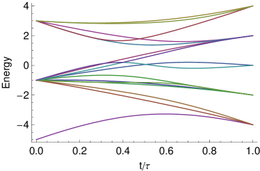
Figure 3: Instantaneous energy spectrum of the five-spin system depicted in figure 1. For simplicity we have omitted the energy levels that are not reachable from the ground state due to different symmetry properties.

Some of the excited states reach the final ground state as $t/\tau\to 1$. In particular, the instantaneous ground state configurations have been found to be continuously connected to a special symmetric combination of four of the final ground states at $t=\tau$, $|2\rangle+|\bar{2}\rangle+|3\rangle+|\bar{3}\rangle$, whereas the other two states $|1\rangle$ and $|\bar{1}\rangle$ are out of reach as long as the system faithfully follows the instantaneous ground state ($\tau\gg 1$). A relatively quick time evolution with an intermediate value of $\tau$ may catch the missed ground states. However, there is no guarantee that the obtained state using this procedure is a true ground state since some of the final excited states may be reached. As shown in the left panel of figure 4, intermediate values of $\tau$ around 10 give almost an even probability to all the true ground states, an ideal situation. However, the problem is that we do not know such an appropriate value of $\tau$ beforehand. In contrast, the right panel of figure 4 shows the result of SA by a direct numerical integration of the master equation, in which all the states are reached evenly in the limit of large $\tau$.

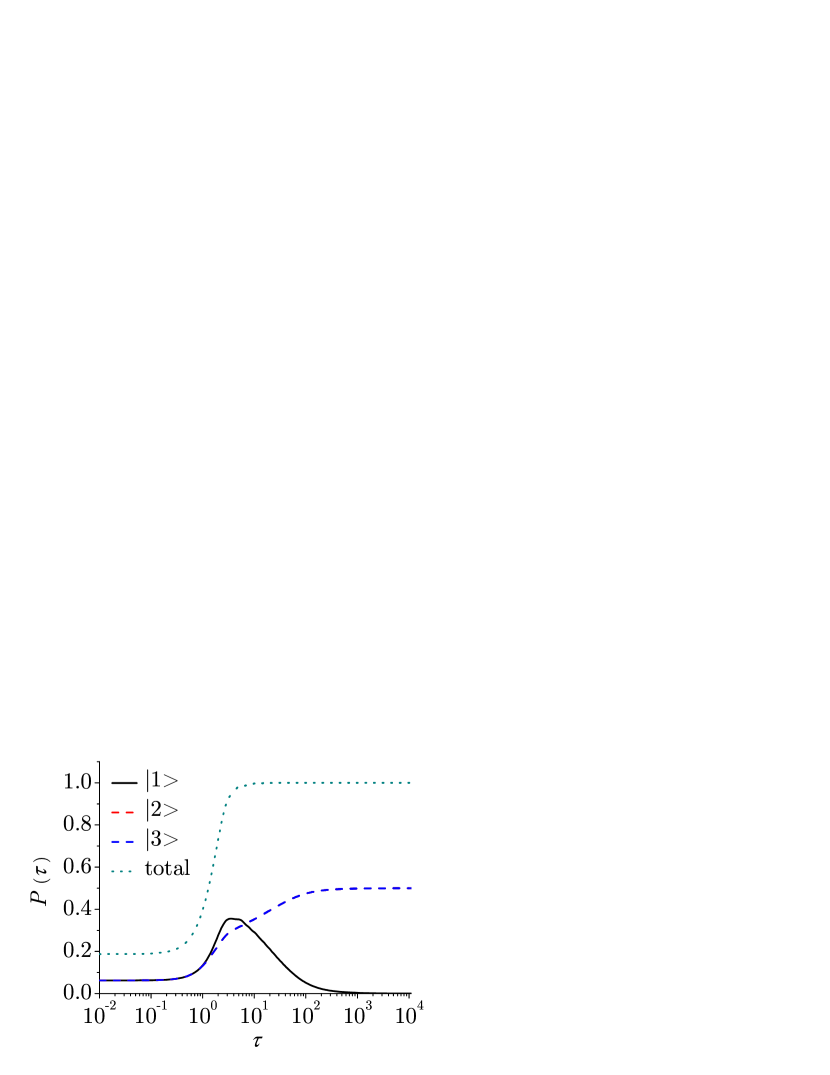
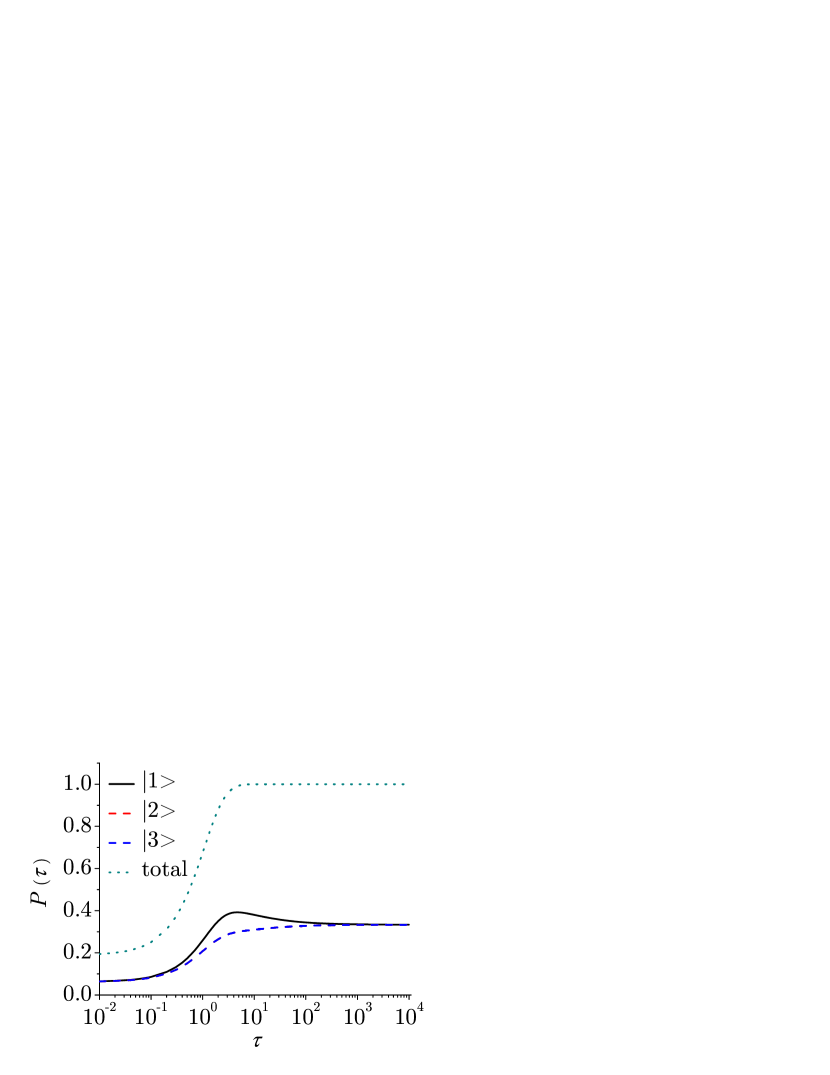
Figure 4: Annealing-time dependence of the final probability that the system is in any one of the ground states. Left panel: Data for the five-spin model using QA. Only the states $|2\rangle$ and $|3\rangle$ (and their reversals $|\bar{2}\rangle$ and $|\bar{3}\rangle$) are reached for large $\tau$. Right panel: SA finds all the states with equal probability.

Figure 3 suggests that it might be plausible to start from one of the low-lying excited states of $H_{1}$ to reach the missed ground state. However, such a process has also been found to cause similar problems as above. We therefore conclude that QA is not suitable to find all degenerate ground-state configurations of the target system $H_{0}$, at least in the present example. This aspect is to be contrasted with SA, in which infinitely-slow annealing of the temperature certainly finds all ground states with equal probability as assured by the theorem of Geman and Geman [11].

QA nevertheless shows astounding robustness against a small perturbation that lifts part of the degeneracy if our interest is in the value of the ground-state energy. Figure 5 depicts the residual energy—the difference between the obtained approximate energy and the true ground-state energy—as a function of the annealing time $\tau$.

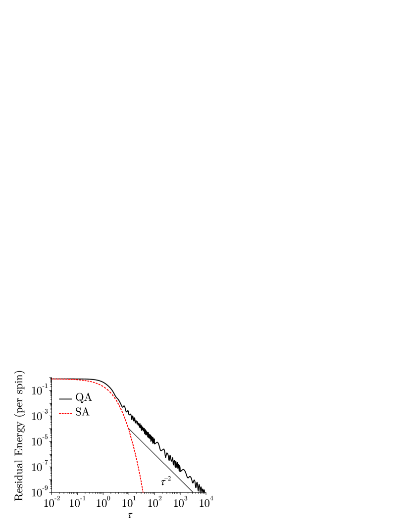
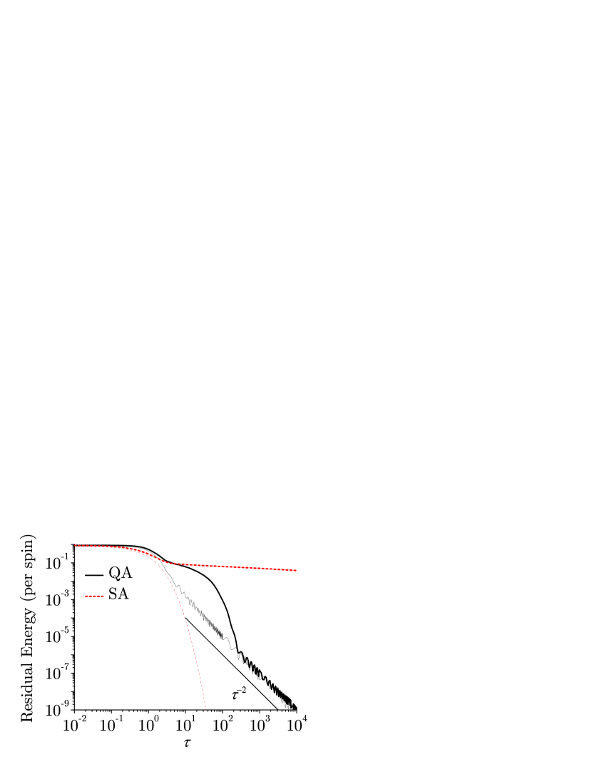
Figure 5: Residual energy per spin as a function of the annealing time $\tau$ for the five-spin toy model. Left panel: Degenerate case. Right panel: A small perturbation $h=0.10$ [see equation (4)] has been added to lift the overall spin-reversal symmetry and thus break the degeneracy. While QA is rather robust against the inclusion of a longitudinal field term and the residual energy per spin decays in both cases $\sim\tau^{-2}$ for large $\tau$, SA seems not to converge after the inclusion of a field term. The thin lines on the right panel represent the results in zero field (from the left panel) for comparison.

Data using SA are also shown in figure 5 using an annealing schedule of temperature $T=(\tau-t)/t$, corresponding to the ratio of the first and the second terms on the right-hand side of equation (3). In the degenerate case (left panel) SA outperforms QA since the residual energy decays more rapidly using SA. However, if we apply a small longitudinal field to $H_{0}$

$$H_{2}=-h\sum_{i=1}^{5}\sigma_{i}^{z}$$ (4)

and regard $H_{0}+H_{2}$ as the target Hamiltonian to be minimized, the situation changes drastically: The convergence of SA slows down significantly while the convergence of QA remains almost intact (right panel of figure 5). As already observed in the simple double-well potential problem [12], the energy barrier between the two almost degenerate states of $H_{0}+H_{2}$ may be too high to be surmountable by SA whereas the width of the barrier remains thin enough to allow for quantum tunnelling to keep QA working.

It is relatively straightforward to modify the type of quantum fluctuations to force the system to finally reach all ground states with equal probability. The following term

$$H_{1}^{\prime}=-\sum\limits_{i}{\sigma_{i}^{x}}-\sum\limits_{\left\langle{i,j}\right\rangle}{\sigma_{i}^{x}\sigma_{j}^{x}}-\sum\limits_{\left\langle{i,j,k}\right\rangle}{\sigma_{i}^{x}\sigma_{j}^{x}\sigma_{k}^{x}}-\cdots$$ (5)

is used instead of $H_{1}$ of equation (2) to induce direct quantum transitions between all states. This modified quantum term is not unnatural in view of the quantum-annealing version of the Grover algorithm [13], in which the quantum term connects all states with equal transition amplitude. The result for the five-spin model is shown in figure 6 (left panel), in which all states are found with equal probability as expected. As depicted in the right panel of figure 6, the scaling of the residual energy still shows the $1/\tau^{2}$ behavior, although an order of magnitude slower. A drawback of this method is that it is not easily implemented by Monte Carlo simulations because of complicated interactions appearing in the path-integral representation of equation (5). We therefore restrict the use of this method to the present section, and Monte Carlo simulations in the next section will be carried out only for the simple transverse-field case of equation (2).

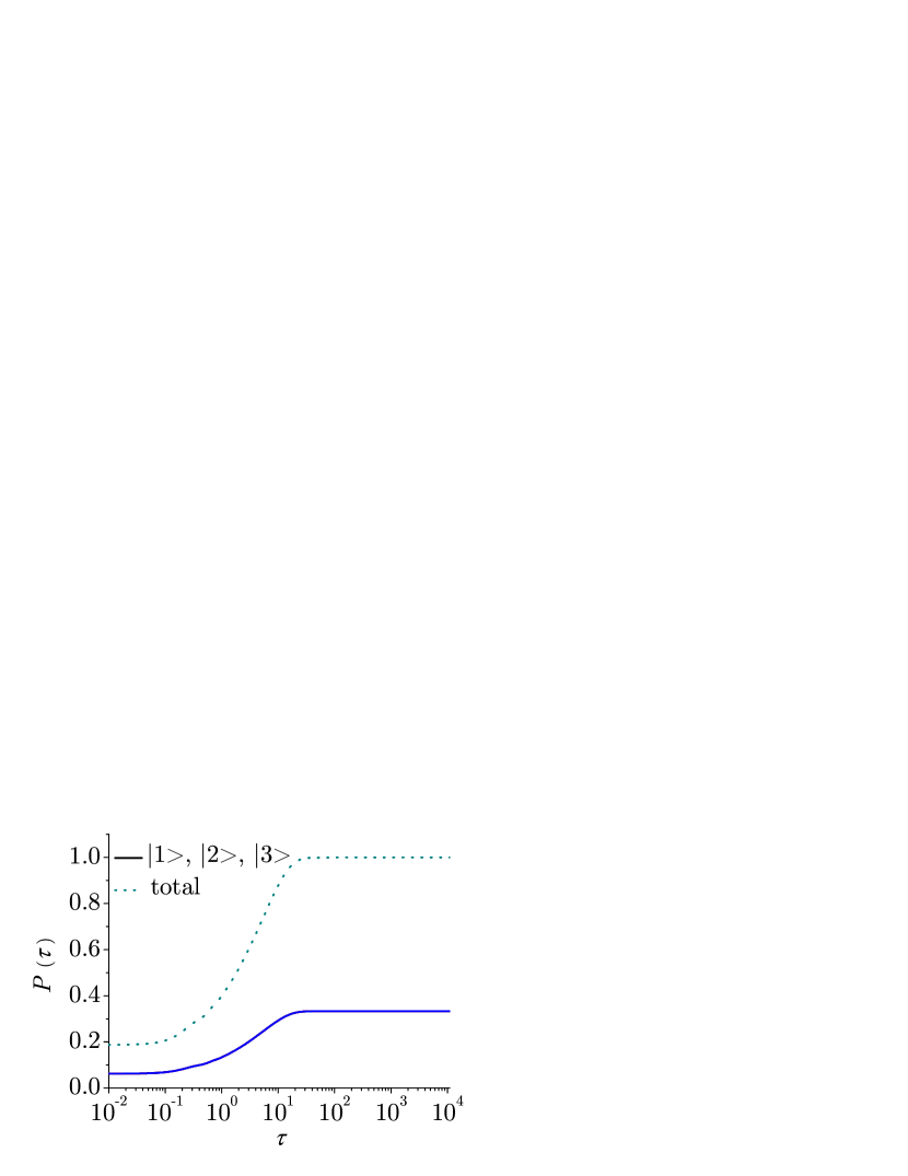
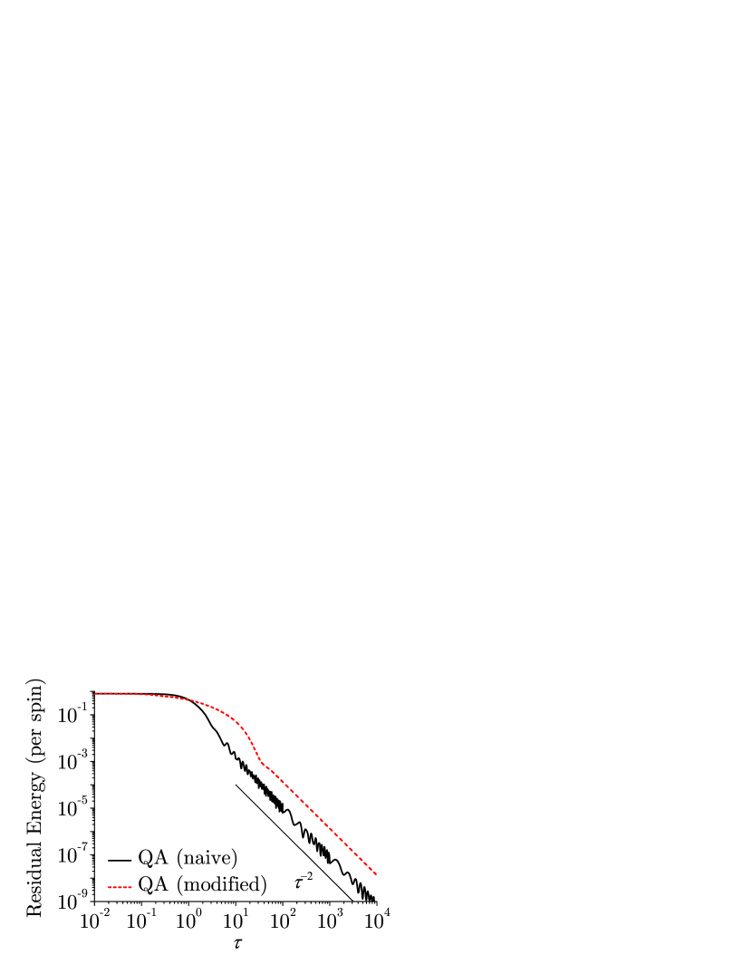
Figure 6: Left panel: Annealing-time dependence of the final probability using the modified Hamiltonian which allows for transitions between states. The data for $\left|1\right\rangle$, $\left|2\right\rangle$ and $\left|3\right\rangle$ fully overlap. Right panel: Residual energy per spin as a function of the annealing time $\tau$ for the modified Hamiltonian. The solid line corresponds to QA using only a transverse field and is depicted for comparison (data from figure 5).

3 Monte Carlo simulations for larger systems

The simplest Ising model which possesses an exponentially-large ground-state degeneracy (in the system size) is the two-dimensional Villain fully-frustrated Ising model [14]. The Ising model is defined on a square lattice of size $N=L\times L$ and has alternating ferromagnetic and antiferromagnetic interactions in the horizontal direction and ferromagnetic interactions in the vertical direction; see figure 7. We use periodic boundary conditions and show the data for $L=4$ and $6$ with $M=1/T=100$, where $M$ is the number of Trotter slices and $T$ the temperature. We follow Ref. [15] and choose $T=1/M$ to ensure an optimal performance of quantum Monte Carlo simulations applied to quantum annealing. A transverse field $H_{1}=-\Gamma\left(t\right)\sum_{i}\sigma_{i}^{x}$ is applied, followed by a pre-annealing of the system by decreasing the temperature as $T=100/Mt$ from $t=0$ to $100$. After the pre-annealing, the transverse field is decreased ($t$ is set to $0$) by the schedule $\Gamma\left(t\right)=(\tau-t)/t$ from $t=0$ to $\tau$ with $T$ fixed. The ground-state energy of the target Hamiltonian $H_{0}$ is given by $-L^{2}$. We can therefore check easily if each Trotter slice has reached one of the ground states.

Figure 7: Fully-frustrated Ising model with $N=36$ spins (dots) and periodic boundary conditions. The system has $45088$ degenerate ground states excluding spin-reversal symmetry. For comparison, for $L=4$ the system has only $136$ degenerate ground states. The horizontal bonds alternate between ferromagnetic (full lines) and antiferromagnetic (dashed lines) signs. The vertical bonds are all ferromagnetic. This ensures that the product of all bonds around any plaquette is negative, i.e., the system is maximally frustrated.

Figures 8 and 9 show the relative number of ground-state hits versus the ground-state numbering (sorted by the number of hits). While a small part of the total set of ground states are reached very frequently, some ground states seem exponentially suppressed in QA. The result is practically independent of the chosen value of the annealing time $\tau$ in the Monte Carlo simulation and coincides with data from the diagonalization of the Hamiltonian corresponding to the adiabatic limit ($\tau\gg 1$) of the Schrödinger dynamics. We may thus conclude that our Monte Carlo simulations with small but finite $T=1/M$ approximate well the final state of the adiabatic Schrödinger equation. In figure 9 we show the relative number of ground-state hits versus the ground-state numbering for SA. In contrast to QA, SA finds almost all ground states with uniform probability. While some ground states seem to be preferred, all ground states can be reached with a frequency of at least 40% (see also Ref. [16]).

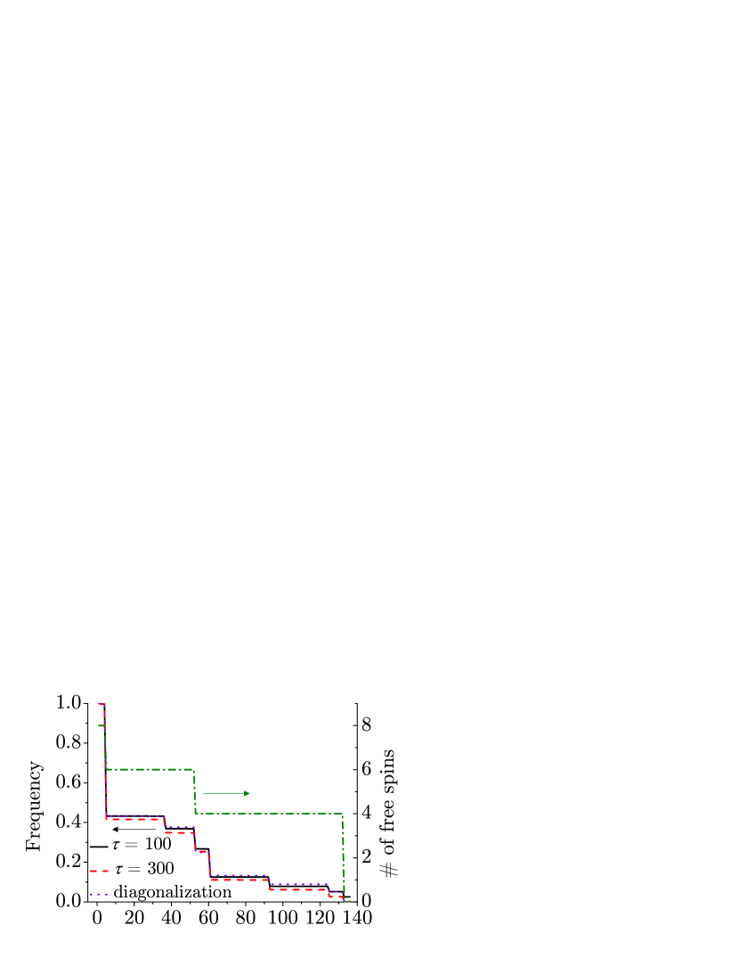
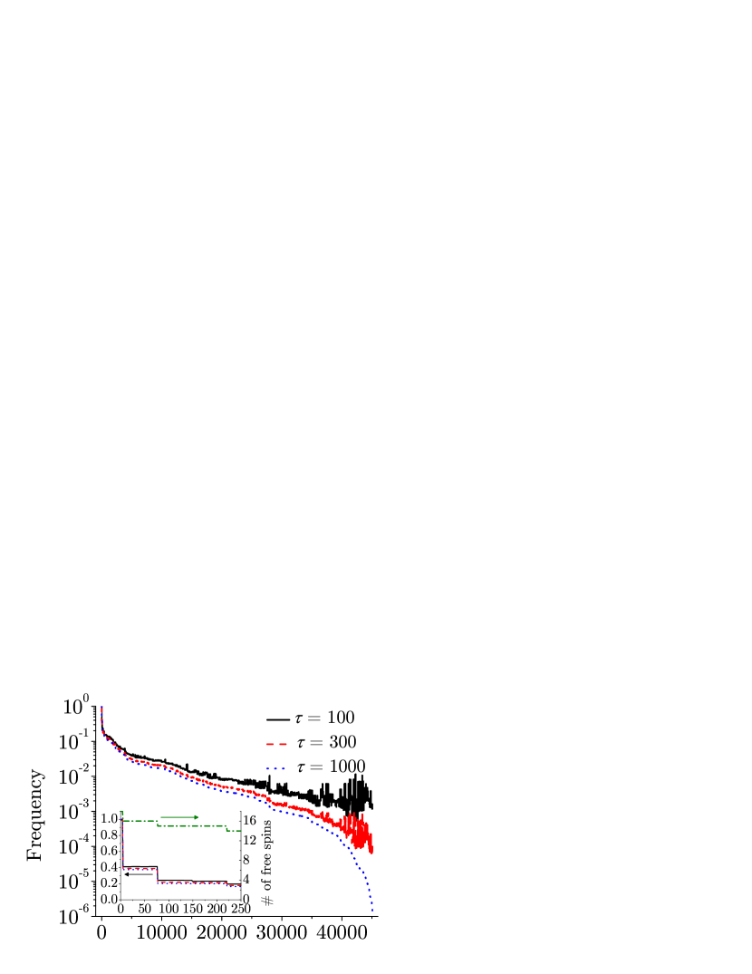
Figure 8: Histograms of the relative frequency that a given ground state is reached by QA. In the abscissa the ground states corresponding to all annealing times are numbered according to the relative frequency of $\tau=300$ for $L=4$ (left panel) and $\tau=1000$ for $L=6$ (right panel) to be reached. The chained lines denote the number of free spins (the spins that can be flipped without energy cost) corresponding to the abscissa. The inset of the right panel is for the high-frequency configurations of the system size $L=6$.

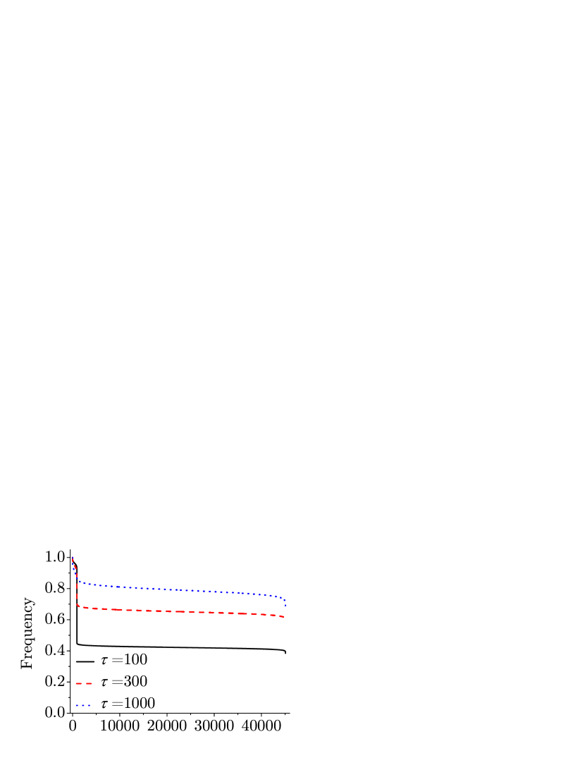
Figure 9: Histograms of the relative frequency by SA. Most ground states are found evenly and all ground states can be reached at least 40% of the time.

It is interesting to study the microscopic configurations of those states with high frequency. Figure 10 shows typical spin configurations of states with high frequency (top panel) and low frequency (bottom panel). The number of free spins (the spins that can be flipped without energy cost) is much larger in the former that in the latter. In figure 8 we also show the number of free spins which clearly shows that the states with more free spins are reached more frequently. A classical ground state with a larger number of free spins would have a lower energy than a state with fewer free spins under a small perturbation of the transverse field because the spins flipped by the transverse field are less likely to be free spins in the latter case with fewer free spins, resulting in high energies. An alternative view is provided if we map a ground-state spin configuration onto a (directed) dimer configuration on the dual lattice by connecting neighbouring plaquettes across an unsatisfied bond [17, 18]. The flip of a free spin in real space corresponds to a dimer plaquette flip. Then the high-frequency configurations in the top panel of figure 10 correspond to dimer configurations with low winding numbers and the low-frequency configurations to large winding numbers ; the former being easier to flip.

We should, however, be careful to assume that these pictures always explains the situation because we have found a counterexample in the $\pm J$ Ising model with $L=10$. A possible reason is that the number of free spins is relatively small for this spin-glass system in comparison with the Villain model, which would lead to weaker effects of spin flips due to quantum fluctuations. Further studies are required to clarify this point.

Figure 10: Typical examples of the high-frequency configurations (top panels) and low-frequency configurations (bottom panels). Filled and open circles denote up and down spins, respectively. Circled spins can be flipped independently without energy changes (free spins).

We next analyze the residual energy. The top two panels of figure 11 show the results for the Villain model with the system size $L=40$ for QA and SA. The abscissa is the annealing time $\tau$ (Monte Carlo steps) multiplied by the number of Trotter slices $M$ for a fair comparison between QA and SA. The left panel is for the average final energy over all Trotter slices and the right panel represents the lowest energy among all Trotter slices. The data for SA follow a rapid decrease beyond $\tau\approx 2\times 10^{3}$, whereas QA (the average energy) stays unimproved beyond this region. While QA for the best energy keeps improving further at lower $T$ (larger $M$), QA does not surpass SA in this annealing time region.

\begin{overpic}[trim=0.0pt 20.075pt 0.0pt 0.0pt,width=433.62pt]{FF_avg.eps} \put(75.0,60.0){Villain}\put(71.0,55.0){(average)} \end{overpic}

\begin{overpic}[trim=0.0pt 20.075pt 0.0pt 0.0pt,width=433.62pt]{FF_best.eps} \put(75.0,60.0){Villain}\put(79.0,55.0){(best)} \end{overpic}

\begin{overpic}[trim=0.0pt 20.075pt 0.0pt 0.0pt,width=433.62pt]{pmJ_avg.eps} \put(82.0,60.0){$\pm J$}\put(71.0,55.0){(average)} \end{overpic}

\begin{overpic}[trim=0.0pt 20.075pt 0.0pt 0.0pt,width=433.62pt]{pmJ_best.eps} \put(82.0,60.0){$\pm J$}\put(79.0,55.0){(best)} \end{overpic}

\begin{overpic}[trim=0.0pt 20.075pt 0.0pt 0.0pt,width=433.62pt]{Gauss_avg.eps} \put(62.0,60.0){Gaussian SG}\put(71.0,55.0){(average)} \end{overpic}

\begin{overpic}[trim=0.0pt 20.075pt 0.0pt 0.0pt,width=433.62pt]{Gauss_best.eps} \put(62.0,60.0){Gaussian SG}\put(79.0,55.0){(best)} \end{overpic}

Figure 11: Residual energy per spin using QA and SA for the Villain model with $L=40$ (top panels), the $\pm J$ model with $L=40$ (middle panels) and the Gaussian spin glass with $L=10$ (bottom panels). The number of samples for the bond randomness is $50$ for the $\pm J$ model and $100$ for the Gaussian model, and the number of runs are over $100$ for the random seedings. We take averages over all samples and calculate the average energy (left panels) and lowest energy (right panels) among all Trotter slices. Errors are smaller than the symbols.

Finally, we also show the data for the two-dimensional $\pm J$ Ising spin glass (middle panels) and Gaussian spin glass with a weak longitudinal field ($h=0.1$) (bottom panels) in order to remove a trivial degeneracy. In fact, the latter model does not have a ground-state degeneracy whereas the Villain model and the $\pm J$ model have quite a large number of ground states. In the $\pm J$ and the Gaussian cases the situation is quite different, since the residual energy using QA decreases more rapidly than SA. Furthermore, the performance of QA improves for smaller $T$ (larger $M$) in the large-$\tau$ region. At high temperature annealing (smaller $M$) it seems that the data of QA are saturated for large $\tau$. This saturation may reflect the finiteness of the temperature of QA. For the $\pm J$ and Gaussian models it seems that QA is a powerful tool, as witnessed in previous studies [1, 4, 5, 6, 7, 8, 15].

4 Conclusion

We have studied the performance of QA for systems with degeneracy in the ground state of the target Hamiltonian. Our results show that naive QA with quantum effects induced by a transverse field reaches only a limited part of the set of degenerate ground-state configurations and misses the other states. The instantaneous energy spectrum as a function of time, figure 3, is a useful tool to understand the situation: some of the excited states merge into the final ground states as $t/\tau\to 1$. It is usually difficult, however, to initially select the appropriate excited states which reach the ground state when $t/\tau\to 1$. We therefore have to be biased a priori in the state search by QA for degenerate cases. An introduction of quantum transitions to all other states significantly improves the situation, leading to a uniform probability to find degenerate ground states, but with the penalty of slower convergence. Simulations of the two-dimensional Villain model show that certain ground-state configurations are exponentially suppressed when using QA, whereas this is not the case for SA. It has been found that the number of free spins is closely related to the frequency that the ground states are found by QA. A ground state with a larger number of free spins is more stable than the others. On the other hand, if the problem is to only determine the ground-state energy, QA is often (but not necessarily always) an efficient method, as exemplified in figures 5 and 11 where the residual energies are shown. Thus, it is necessary to construct an analytical theory—based on the numerical evidence—to establish criteria when to (and when not to) use QA.

References

References

- [1] Kadowaki T and Nishimori H 1998 Phys. Rev. E 58 5355
- [2] Finnila A B, Gomez M A, Sebenik C, Stenson C and Doll J D 1994 Chem. Phys. Lett. 219 343
- [3] Kirkpatrick S, Gelatt, Jr C D and Vecchi M P 1983 Science 220 671
- [4] Das A and Chakrabarti B K 2005 Quantum Annealing and Related Optimization Methods (Edited by A. Das and B.K. Chakrabarti, Lecture Notes in Physics 679, Berlin: Springer)
- [5] Santoro G, Martoňák R Tosatti E and Car R 2002 Science 295 2427
- [6] Martoňák R, Santoro G E and Tosatti E 2002 Phys. Rev. B 66 094203
- [7] Santoro G E and Tosatti E 2006 J. Phys. A 39 R393
- [8] Das A and Chakrabarti B K 2008 Rev. Mod. Phys. 80 1061
- [9] Young A P, Knysh S and Smelyanskiy V N 2008 Phys. Rev. Lett. 101 170503
- [10] Morita S and Nishimori H 2008 J. Math. Phys. 49 125210
- [11] Geman S and Geman D 1984 IEEE Trans. Pattern. Analy. Mach. Intell. PAMI-6 721
- [12] Stella L, Santoro G E and Tosatti E 2005 Phys. Rev. B 72 014303
- [13] Roland J and Cerf N J 2002 Phys. Rev. A 65 042308
- [14] Villain J 1977 J. Phys. C 10 1717
- [15] Kadowaki T 1998 Study of Optimization Problems by Quantum Annealing Ph.D. thesis Tokyo Institute of Technology (quant-ph/0205020)
- [16] Moreno J J, Katzgraber H G and Hartmann A K 2003 Int. J. Mod. Phys. C 14 285
- [17] Moessner R and Sondhi S L 2001 Phys. Rev. Lett. 86 1881
- [18] Moessner R and Sondhi S L 2003 Phys. Rev. B 68 184512