On implicit ODEs with hexagonal web of solutions

Abstract

Solutions of an implicit ODE form a web. Already for cubic ODEs the 3-web of solutions has a nontrivial local invariant, namely the curvature form. Thus any local classification of implicit ODEs necessarily has functional moduli if no restriction on the class of ODEs is imposed. Here the most symmetric case of hexagonal 3-web of solutions is discussed, i.e. the curvature is supposed to vanish identically. A finite list of normal forms is established under some natural regularity assumptions. Geometrical meaning of these assumptions is that the surface, defined by ODE in the space of 1-jets, is smooth as well as the criminant, which is the critical set of this surface projection to the plane.

Key words: implicit ODE, hexagonal 3-web, equivariant diffeomorphism.

AMS Subject classification: 37C15 (primary), 53A60, 37C80 (secondary).

1 Introduction

Consider an implicit ordinary differential equation

$$F(x,y,p)=0$$ (1)

with a smooth or real analytic $F$. This ODE defines a surface $M$:

$$M:=\{(x,y,p)\in{\mathbb{R}^{2}\times\mathbb{P}}^{1}(\mathbb{R}):\ F(x,y,p)=0\},$$ (2)

where $(x,y,p)$ are coordinates in the jet space $J^{1}(\mathbb{R},\mathbb{R})$ with $p=\frac{dy}{dx}$. Generically the condition $\left.{\rm grad}(F)\right|_{F(x,y,p)=0}\neq 0$ holds true for any point $m=(x,y,p)\in M$, i.e. $M$ is smooth. If the projection $\pi:M\to\mathbb{R}^{2},\ (x,y,p)\mapsto(x,y)$ is a local diffeomorphism at a point $m\in M$ then this point is called regular. In some neighborhood of the projection of a regular point $\pi(m)$ equation (1) can be solved for $p$ thus defining an explicit ODE.

If the projection $\pi$ is not a local diffeomorphism at $m$, then the point $m$ is called a singular point of implicit ODE (1). The set of all singular points is called the criminant of equation (1) or the apparent contour of the surface $M$ and will be denoted by $C$:

$$C:=\{(x,y,p)\in\mathbb{R}^{2}\times\mathbb{P}^{1}(\mathbb{R}):F(x,y,p)=F_{p}(x,y,z)=0\},$$ (3)

where the low subscript denotes a partial derivative: $F_{p}=\frac{\partial F}{\partial p}$.

Studying of generic singular points of implicit ODEs was initiated by Thom in [26]. Due to Whitney’s Theorem such points are folds and cusps of the projection $\pi$. Local normal forms for generic singularities were conjectured by Dara in [11] and for a generic fold point were established by Davydov in [12]. The classification list for a generic fold point of the projection $\pi$ is exhausted by a well folded saddle point, a well folded node point, a well folded focus point and the regular singular point, where contact plane is transverse to the criminant. Cusp points were studied by Dara [11], Bruce [7] and Hayakawa, Ishikawa, Izumiya, Yamaguchi [20].
Usually the following regularity condition is imposed at each point of the criminant:

$${\rm rank}((x,y,p)\mapsto(F,F_{p}))=2.$$ (4)

This regularity condition implies that the criminant is a smooth curve. At each point $m$ outside the criminant $C$ the contact plane $dy-pdx=0$ cuts the tangent plane $T_{m}M$ along a line thus giving a direction field, which takes the form:

$$\tau=[F_{p}:pF_{p}:-(F_{x}+pF_{y})],$$ (5)

in the coordinates $(x,y,p)$. This direction field is called the characteristic field of $M$. The projection $\pi(\gamma)$ of an integral curve $\gamma\subset M$ of the characteristic field $\tau$ is called a solution of ODE (1). If $F_{pp}\neq 0$ at a point $m\in C$ on the criminant then (1) reduces locally to quadratic in $p$ (or binary) ODE. Such equations were the subject of intensive study. See, for example, [8],[9],[10],[19].

Suppose equation (1) has a triple root $p_{0}$ at $(x_{0},y_{0})$ then the equation $F=0$ can be written locally as a cubic equation

$$p^{3}+a(x,y)p^{2}+b(x,y)p+c(x,y)=0,$$ (6)

as follows from the Division Theorem. Thus if in a domain $U\subset\mathbb{R}^{2}$ outside the discriminant curve $\Delta:=\pi(C)$ this cubic equation has 3 real roots $p_{1},p_{2},p_{3}$, we have 3-web formed by solutions of (1). A generic 3-web has a nontrivial invariant. In differential-geometric conext this invariant is the curvature form of the web. Therefore any general local classification of cubic implicit ODEs (6) necessarily has functional moduli (cf. [12]). Moreover, this invariant is topological in nature hence even topological classification will have functional moduli if no restriction is imposed on the class of ODE. (See also [22] and [23], where web structure was used for studying geometric properties of differential equations.)

In this paper we consider cubic ODEs (6) with a hexagonal web of solutions. Equations of this type describe, for example, webs of characteristics on solutions of integrable systems of three PDEs of hydrodynamic type (see [14], [15]). Another example is WDVV associativity equation (see Example 2 below).

Definition 1

Let $U\subset\mathbb{R}^{2}$ be the open set, where (6) has 3 real roots $p_{1},p_{2},p_{3}$ and suppose $U\neq\emptyset$. We say that (6) has a hexagonal 3-web of solutions if for the projection $\pi(m)$ of each regular point $m\in M$ with $\pi(m)\in U$ there is a local diffeomorphism at $\pi(m)$ mapping the solutions of (6) to three families of parallel lines.

The case of hexagonal web of solutions is also the most symmetric, i.e. the Lie symmetry pseudogroup of (1) at a regular point has the largest possible dimension 3. The list of normal forms turnes out to be finite provided regularity condition (4) is satisfied. These forms are given by the following examples.

Example 1

The classical Graf and Sauer theorem [18] claims that a 3-web of straight lines is hexagonal iff the web lines are tangents to an algebraic curve of class 3, i.e. the dual curve is cubic. This implies immediately that the following cubic Clairaut equation has a hexagonal 3-web of solutions:

$$p^{3}+px-y=0.$$ (7)

The solutions are the lines $p=const$ enveloping a semicubic parabola. (See Fig. 1) Note that the contact plane is tangent to $M$ along the criminant, i.e. the criminant is a Legendrian curve.

Example 2

Consider associativity equation

$$u_{xxx}=u^{2}_{xyy}-u_{xxy}u_{yyy},$$

describing 3-dimensional Frobenius manifolds (see [13]). Each of its solutions $u(x,y)$ defines a characteristic web in the plane, which is hexagonal as was shown by Ferapontov [16]. Characteristics are integral curves of the vector field

$$\partial_{x}-\lambda(x,y)\partial_{y},$$

where $\lambda$ satisfy the characteristic equation

$$\lambda^{3}+u_{yyy}\lambda^{2}-2u_{xyy}\lambda+u_{xxy}=0.$$

For the solution $u=\frac{x^{2}y^{2}}{4}+\frac{x^{5}}{60}$ the characteristic equation becomes

$$p^{3}+2xp+y=0$$ (8)

after the substitution $x\to-x$, $y\to-y$, $\lambda\to-p$. The criminant of this ODE is not Legendrian and the solutions have ordinary cusps on the discriminant (see Fig. 1). The discriminant is also a solution. In the analytic setting the above two normal forms were conjectured by Nakai in [24].

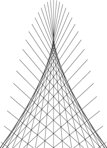
Figure 1: Solutions of $p^{3}+px-y=0$ (left) and $p^{3}+2xp+y=0$ (right) with horizontal y-axis.

We find also local normal forms at points, where the projection $\pi$ has a fold, i.e. the cubic ODE factors out to a quadratic and a linear terms.

Example 3

Suppose the criminant of ODE is Legendrian then this ODE is locally equivalent to

$$p^{2}=y.$$ (9)

Solutions of this ODE together with the lines $dx=0$ form a hexagonal 3-web (see Fig. 1). In fact, both the lines $dy=0$ or the parabolas $2dy-xdx=0$ also supplement the 2-web of solutions of (9) to a hexagonal 3-web, but the surfaces of the corresponding cubic equations $p(p^{2}-y)=0$ and $(2p-x)(p^{2}-y)=0$ are not smooth at $m=(0,0,0)$. If we agree to consider a quadratic equation as a cubic with one root at infinity, than equation (9) is the third normal form in our list. The following coordinate change $y=\tilde{y}+\frac{\tilde{x}^{2}}{4}$, $x=\tilde{x}$ straightens the solutions, transforming ODE (9) to a quadratic Clairaut equation

$$\tilde{p}^{2}+\tilde{p}\tilde{x}-\tilde{y}=0.$$

As the the lines $dx=0$ are preserved this example is also a special case of the Graf and Sauer Theorem.

Example 4

Suppose the criminant of ODE is not Legendrian then this ODE is locally equivalent to

$$p^{2}=x.$$ (10)

Solutions of this ODE together with the lines $dx=0$ form a hexagonal web (See Fig. 2). The lines $dy=0$ also complete the 2-web of solutions of (10) to a hexagonal 3-web, but again the surface $M$ of the corresponding cubic equation $p(p^{2}-x)=0$ is not smooth at $m=(0,0,0)$.

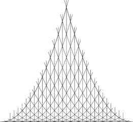
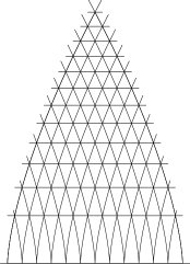
Figure 2: Solutions of $p^{2}=y$ and the lines $dx=0$ (left). Solutions of $p^{2}=x$ and the lines $dx=0$ with horizontal y-axis (right).

Example 5

For completeness let us mention the case of a regular point of an implicit cubic ODE. If its 3-web of solutions is hexagonal it can be mapped to the web of 3 families of parallel lines $dx=0$, $dy=0$ and $dx+dy=0$. This gives the following ”cubic” ODE

$$p(p+1)=0.$$ (11)

Now we can formulate our classification theorem.

Theorem 1

Suppose functions $a,b,c$ are real analytic and the following conditions hold for an implicit cubic ODE

$$F(x,y,p):=p^{3}+a(x,y)p^{2}+b(x,y)p+c(x,y)=0$$

at a point $m=(x_{0},y_{0},p_{0})\in M:=\{(x,y,p)\in{\mathbb{R}^{2}\times\mathbb{P}}^{1}(\mathbb{R}):\ F(x,y,p)=0\}$:
1) this equation has a hexagonal 3-web of solutions,
2) $dF|_{m}\neq 0$,
3) ${\rm rank}((x,y,p)\mapsto(F,F_{p}))|_{m}=2$ if $m$ lies on the criminant $C$.
Then this ODE is equivalent to one of the following five forms with respect to some local real analytic isomorphism:

$$\begin{array}[]{ll}i)\ \ \ p^{3}+2xp+y=0,&\mbox{if $p_{0}$ is a triple root and the criminant is transverse to the}\\ &\mbox{ contact plane field in some punctured neighborhood of $m$,}\\ ii)\ \ \ p^{3}+px-y=0,&\mbox{if $p_{0}$ is a triple root and the criminant is Legendrian,}\\ iii)\ \ p^{2}=y,&\mbox{if $p_{0}$ is a double root and the criminant is Legendrian,}\\ iv)\ \ p^{2}=x,&\mbox{if $p_{0}$ is a double root and the criminant is transverse}\\ &\mbox{to the contact plane at $m$,}\\ v)\ \ \ p(p+1)=0,&\mbox{if the roots are pairwise distinct at $\pi(m)=(x_{0},y_{0})$.}\\ \end{array}$$ (12)

If the functions $a,b,c$ are smooth and conditions 1),2),3) are satisfied then there is a diffemorphism of a neighborhood of the point $(x_{0},y_{0})$ onto a neighborhood of the point $(0,0)$ reducing the above cubic ODE either to one of the four equations (12ii)-(12v) or to an equations that coincides with (12i) within the domain, where (12i) has three real roots.

The main difficulty in proving the above classification theorem brings the case of irreducible cubic ODE. The idea is to lift its 3-web of solutions to $M$ and then to the plane $E:\ p_{1}+p_{2}+p_{3}=0$ in the space of roots of the cubic equation $p^{3}+A(x,y)p+B(x,y)=0$. (Note that the general case reduces to this cubic.) Then this 3-web at the plane $E$ has $\mathbb{D}_{3}$-symmetry permuting the roots. Using the regularity condition we construct a $\mathbb{D}_{3}$-equivariant diffeomorphism ”upstairs”, matching the web to that of a corresponding normal form. Due to the $\mathbb{D}_{3}$-symmetry the constructed diffeomorphism is lowerable to some diffeomorphism ”downstairs”, i.e. to a point transformation in the plane of solutions. Most of the claims and the proofs below are given for the smooth case and for some neighborhood of the projection $\pi(m)$ of $m\in M$, if it is not stated explicitly. In section 4 we discuss how to get rid of the annoying stipulation in Theorem 1 for the smooth case (12i) by replacing Definition 1 with a less geometric one.

2 Normal forms for a fold point

In this section we establish normal forms for the case, when the projection $\pi$ has a fold point at $m$. If cubic equation (6) has two coinciding roots then the the third root defines a regular point of the projection $\pi$ and the equation factors to a quadratic equation and a linear one. Regularity condition (4) for a double root $p_{0}$ implies immediately that the projection $\pi$ has a fold point at $m$. First we find a normal form for fold points and the symmetries of this normal form. Further we look for the linear in $p$ (i.e. explicit) equation whose solutions complete the 2-web of solutions of the quadratic normal form to a hexagonal 3-web. Finally, we bring these linear terms to some normal forms using the symmetries of the quadratic equation. We start with a Legendrian criminant, then consider non-Legendrian criminant and finally show that the case of an isolated point of tangency of the criminant and the contact plane is excluded by the regularity conditions.

2.1 The case of Legendrian criminant

Proposition 1

Consider implicit ODE (1) with a smooth Legendrian criminant and a smooth surface (2). Then characteristic field (5) can be smoothly extended to the criminant. Moreover, the extended characteristic field is transverse to the criminant.

Proof: Let $m$ be a point on the criminant. A suitable contactomorphism $\varphi$ maps $M$ to $M^{\prime}$ with the following properties:
a) the criminant of $M$ is mapped to the line $x=y=0$,
b) $\varphi(m)=(0,0,0)$,
c) the tangent plane $T_{m}M$ is mapped to the plane $y=0$.
It suffices to prove the proposition for the transformed surface $M^{\prime}:=\{(x,y,p)\in\mathbb{R}^{2}\times\mathbb{P}^{1}(\mathbb{R}):G(x,y,p)=0\}$ with the Legendrian line $x=y=0$. Condition c) allows to rewrite $G(x,y,p)=0$ as

$$y=g(x,p),$$

while condition a) implies $g(x,p)=xf(x,p)$. Now $g_{p}(0,0)=g_{x}(0,0)=0$ implies $f(0,0)=0$, so that $f(x,p)=pu(x,p)+xv(x,p)$ by the Hadamard lemma. As the line $x=y=0$ is Legendrian, the form $dy-pdx$ must vanish on it: $\left.\{d(xpu(x,p)+x^{2}v(x,p))-pdx\}\right|_{x=0}=\left.\{(pu(x,p)dx-pdx\}\right|_{x=0}=0$ or $u(0,p)\equiv 1$. Again by the Hadamard lemma one gets $u(x,p)=1+xw(x,p)$ and

$$y=xp+x^{2}h(x,p)$$

with $h(x,p)=pw(x,p)+v(x,p)$. Now the characteristic field $\tau$ is defined by restriction of equation $dy-pdx=0$ to $M^{\prime}$, i.e. by $\left.\{d(xp+x^{2}h(x,p))-pdx\}\right|_{M^{\prime}}=x\{(1+xh_{p}(x,p))dp+(2h(x,p)+xh_{x}(x,p))dx\}=0$. This implies that the characteristic field on $M^{\prime}$ in coordinates $(x,p)$ is generated by the vector field $(1+xh_{p}(x,p))\partial_{x}-(2h(x,p)+xh_{x}(x,p))\partial_{p}$ which is clearly smooth and transverse to the line $x=y=0$ on $M^{\prime}$.

$\Box$

Theorem 2

Let (1) be an implicit ODE such that corresponding surface (2) is smooth. Suppose its criminant $C$ is a smooth Legendrian curve and the projection $\pi:(x,y,p)\to(x,y)$ has a fold singularity at $m\in C$. Then (1) is locally equivalent to

$$p^{2}=y$$ (13)

with respect to some diffeomorphism $\varphi:\tilde{U}\to U$, where $\tilde{U},U\in\mathbb{R}^{2}$ are neighborhoods of $(0,0)$, $\pi(m)$ and $\varphi(0,0)=\pi(m)$.

Proof: Due to Proposition 1 there is a smooth direction field $\tau$ on $M$. Its integral curves define a foliation $\mathcal{F}$ of a neighborhood of $m$. As the projection $\pi$ has a fold on the criminant, the discriminant curve $\Delta=\pi(C)\in\mathbb{R}^{2}$ is smooth. Let us choose new coordinates on $(U,\pi(m))$ such that the discriminant curve turns to the line $y=0$. Then equation (1) is equivalent to $y=g(x,p)$. The discriminant curve is a solution therefore $g(x,p)=pf(x,p)$ by the Hadamard lemma. The criminant $y=p=0$ is Legendrian hence $\{d(pf(x,p))-pdx\}_{p=0}=f(x,0)dp=0$ or $f(x,0)\equiv 0$. Now $f(x,p)=ph(x,p)$ and $y=p^{2}h(x,p)$. As the projection $\pi$ has a fold at $m\in M$ holds true $\left.{\partial_{p}^{2}}(p^{2}h(x,p))\right|_{x=p=0}=2h(0,0)\neq 0$. Consequently characteristic field (5) on $M$ with $F(x,y,p)=p^{2}h(x,p)-y$ is generated by the vector field

$$(2ph(x,p)+p^{2}h_{p}(x,p))\partial_{x}-(p^{2}h_{x}(x,p)-p)\partial_{p}=p\{(2h(x,p)+ph_{p}(x,p))\partial_{x}+(1-ph_{x}(x,p))\partial_{p}\}.$$

Due to $h(0,0)\neq 0$ it is transverse to the kernel of $d\pi$ on $M$ hence the projection of each integral curve crossing the criminant $C$ is smooth and tangent to the discriminant curve. Locally the equation $p^{2}h(x,p)-y=0$ can be rewritten as a quadratic equation

$$p^{2}+a(x,y)p+b(x,y)=0.$$

This easily follows from the Division Theorem since $h(0,0)\neq 0$. Moreover, as the criminant $y=p=0$ is a Legendrian curve holds true $b(x,0)=a(x,0)=0$. Thus one gets $a(x,y)=y\alpha(x,y)$ and $b(x,y)=y\beta(x,y)$ with $\beta(0,0)\neq 0$ as $M$ is smooth at $m=(0,0,0)$. Consider $(x,p)$ as local coordinates on $M$ and define the map $i:M\to M$ by

$$i(x,p)=(x,-p-p^{2}h(x,p)\alpha(x,p^{2}h(x,p))).$$ (14)

This map is the involution that permutes the roots $p_{1},p_{2}$ of our quadratic ODE. Let the foliation $\mathcal{F}$ on $M$ be defined locally by $I(x,p)=const$ with $\left.{\rm grad}(I)\right|_{x=p=0}\neq 0$, where $I$ is a first integral of the characteristic field $\tau$. Then the functions $I$ and $J:=i^{*}(I)$ are functionally independent as $di(\tau)$ and $\tau$ are transverse to each other. Since $\tau$ is transverse also to the criminant the partial derivative $\left.I_{x}\right|_{x=p=0}$ does not vanish. Hence one can chose $I$ so that $I(x,0)=x$ which implies $J(x,0)=x$. Let us take thus normalized functions $I,J$ as local coordinates on $M$. Note that the following relation holds true

$$\pi(I,J)=\pi(J,I),$$ (15)

since $i(I,J)=(J,I)$. For the ODE $\tilde{p}^{2}=\tilde{y}$ the above defined objects are as follows: $\tilde{I}(\tilde{x},\tilde{p})=\tilde{x}-2\tilde{p}$, $\tilde{i}(\tilde{x},\tilde{p})=(\tilde{x},-\tilde{p})$, $\tilde{J}(\tilde{x},\tilde{p})=\tilde{x}+2\tilde{p}$. Now define a diffeomorphism germ $\psi:\tilde{M},0\to M,0$ by $\psi(\tilde{I},\tilde{J})=(\tilde{I},\tilde{J})$. By (15) there exists such a map germ $\varphi:\mathbb{R}^{2},0\to\mathbb{R}^{2},0$ that the following diagram commutes:

$$\begin{array}[]{ccc}M,0&\stackrel{{\scriptstyle\psi}}{{\longleftarrow}}&\tilde{M},0\\ \downarrow\pi&&\downarrow\tilde{\pi}\\ \mathbb{R}^{2},0&\stackrel{{\scriptstyle\varphi}}{{\longleftarrow}}&\mathbb{R}^{2},0\\ \end{array}$$ (16)

We claim that the map germ $\varphi$ is the searched for diffeomorphism. By construction it maps solutions to solutions. To show that $\varphi$ is differentiable consider the map germ $\pi\circ\psi:\tilde{M},0\to\mathbb{R}^{2},0$. Applying Malgrange’s Preparation Theorem to this map germ in coordinates $(\tilde{x},\tilde{p})$ on $\tilde{M},0$ and $(x,y)$ on $\mathbb{R}^{2},0$ one gets

$$x=X_{0}(\tilde{x},\tilde{p}^{2})+\tilde{p}X_{1}(\tilde{x},\tilde{p}^{2}),\ \ y=Y_{0}(\tilde{x},\tilde{p}^{2})+\tilde{p}Y_{1}(\tilde{x},\tilde{p}^{2}),$$

where the functions $X_{0},X_{1},Y_{0},Y_{1}$ are smooth. Since $\pi\circ\psi(\tilde{x},\tilde{p})=\pi\circ\psi(\tilde{x},-\tilde{p})=(x,y)$ holds true $X_{1}(\tilde{x},\tilde{p}^{2})=Y_{1}(\tilde{x},\tilde{p}^{2})=0$. With $\tilde{p}^{2}=\tilde{y}$ the above formulas take the form

$$x=X_{0}(\tilde{x},\tilde{y}),\ \ y=Y_{0}(\tilde{x},\tilde{y}),$$

and therefore define a smooth map germ $\varphi$. Applying the same considerations to the map germ $\tilde{\pi}\circ\psi^{-1}$ we see that $\psi$ has an inverse for $y\geq 0.$ Therefore $\psi$ is invertible.                           $\Box$

Remark. Note that equation (13) has a nontrivial symmetry group. For example, the scaling $x\to\lambda x,\ \ y\to\lambda^{2}y$ leaves it invariant. Therefore the diffeomorphism $\varphi$ in Theorem 2 is not unique.

Proposition 2

Equation (13) has an infinite symmetry pseudogroup. Its transformations are given by

$$\tilde{x}=F(x+2\sqrt{y})+F(x-2\sqrt{y}),\ \ \tilde{y}=\frac{1}{4}[F(x+2\sqrt{y})-F(x-2\sqrt{y})]^{2}.$$ (17)

Here $F$ is a smooth function subjected to $\left.F^{\prime}(u)\right|_{u=0}\neq 0$. Infinitesimal generators of this pseudogroup have the form

$$\{f(x+2\sqrt{y})+f(x-2\sqrt{y})\}\partial_{x}+\sqrt{y}\{f(x+2\sqrt{y})-f(x-2\sqrt{y})\}\partial_{y},$$ (18)

where $f$ is an arbitrary smooth function.

Proof: Consider the action of symmetry group transformation on $M$ in coordinates $(u,v)$, where

$$u=x-2p,\ \ v=x+2p.$$ (19)

To preserve the foliations $\mathcal{F}$ and $i(\mathcal{F})$ determined by the direction fields $\tau$ and $di(\tau)$ it must have the following form $\bar{u}=2F(u),\ \bar{v}=2G(v)$. This transformation is a symmetry if it commutes with $i$. Note that $i$ permutes $u$ and $v$ and sends $\partial_{p}$ to $-\partial_{p}$. Hence $F=G$. Now substitutions $\bar{x}=\frac{1}{2}(F(v)+F(u))$ and $\bar{y}=\bar{p}^{2}=\frac{1}{4}(F(v)+F(u))^{2}$ gives (17). Condition $\left.F^{\prime}(u)\right|_{u=0}\neq 0$ is equivalent to non-vanishing of the Jacobian: $\left.\frac{\partial(\tilde{x},\tilde{y})}{\partial(x,y)}\right|_{x=y=0}\neq 0.$

Consider now infinitesimal symmetries of (13). They are defined by operators $\xi(x,y)\partial_{x}+\eta(x,y)\partial_{y}$. These operators must be liftable to $M$. On $M$ the lifted vector field must be a symmetry of foliations $\mathcal{F}$ and $i(\mathcal{F})$. In coordinates $(u,v)$ any infinitesimal symmetry $X$ of foliations $\mathcal{F}$ and $i(\mathcal{F})$ is easy to write down:

$$X=f(u)\partial_{u}+g(v)\partial_{v}.$$ (20)

In coordinates $(x,p)$ on $M$ this operator $X$ takes the form

$$X=\frac{1}{2}(g(v)+f(u))\partial_{x}+\frac{1}{4}(g(v)-f(u))\partial_{p}.$$

$X$ is lowerable iif $di(X)=X$. Now lowerability condition amounts to $f(u)+g(v)=f(v)+g(u)$ and $g(v)-f(u)=f(v)-g(u)$. Thus the first equation gives $f(u)-g(u)=c=const$ and the second implies $c=0$. Substitution $u=x-2\sqrt{y}$, $v=x+2\sqrt{y}$, $p=\sqrt{y}$ into $X$ gives (18) for $y>0$. The obtained transformations are correctly defined for $y>0$ and are smoothly (analytically) extendable for $y\geq 0$. The possibility to extend them for $y\leq 0$ easily follows from Malgranges’s Preparation Theorem: one considers the projection $\pi:M\to\mathbb{R}^{2}$, $(x,p)\mapsto(x,p^{2})$ in coordinates $x,p$ on $M$ and $x,y$ on $\mathbb{R}^{2}$ and observes that $F(x+2p)+F(x-2p)$ is an even and $F(x+2p)-F(x-2p)$ is an odd function with respect to $p$.

$\Box$

To use the above symmetries we need the following lemma.

Lemma 1

If a smooth (analytic) function germ $f:\mathbb{R},0\to\mathbb{R},0$ is not flat then the vector field germ $f(u)\partial_{u}$ on $\mathbb{R},0$ is equivalent to $u^{k}\partial_{u}$ with respect to a certain smooth (analytic) coordinate transformation $\bar{u}=F(u)$, where $k\in\mathbb{N}$ is such that $\left.\frac{d^{k}f(u)}{{du}^{k}}\right|_{u=0}$ is the first non-vanishing derivative at $0$ .

Proof: $F(u)$ must satisfy ODE $f(u)F^{\prime}(u)=(F(u))^{k}$. The existence of $F(u)$ with $F^{\prime}(u)|_{u=0}\neq 0$ is easily verified in both smooth and analytic cases.

$\Box$

Theorem 3

Suppose the solutions of (13) and those of

$$\alpha(x,y)dx+\beta(x,y)dy=0,$$ (21)

where $\alpha(x,y),\beta(x,y)$ are non-flat functions at $(0,0)$, form together a hexagonal 3-web. Then there is a local symmetry of (13) at $(0,0)$ that maps equation (21) to one of the two following forms for $y\geq 0$:

$$\begin{array}[]{c}[(x+2\sqrt{y})^{k}+(x-2\sqrt{y})^{k}]dx-\frac{1}{\sqrt{y}}[(x+2\sqrt{y})^{k}-(x-2\sqrt{y})^{k}]dy=0,\ {\rm or}\\ \\ \sqrt{y}[(x+2\sqrt{y})^{k}-(x-2\sqrt{y})^{k}]dx-[(x+2\sqrt{y})^{k}+(x-2\sqrt{y})^{k}]dy=0,\\ \end{array}$$ (22)

where $k$ is a non-negative integer. In particular, if $\alpha(x,y),\beta(x,y)$ are non-flat functions with $(\alpha(0,0),\beta(0,0))\neq(0,0)$, one gets three normal forms:

$$a)\ dx=0,\ \ \ b)\ dy=0,\ \ \ c)\ 2dy-xdx=0.$$ (23)

Moreover, if equation (21) for $y\geq 0$ is equivalent to (23a) or (23b) then it can be reduced to (23a), respectively (23b) by a symmetry of (13) in some neighborhood of the point $(0,0)$

Proof: Let us introduce operators $U,V$ of differentiation along the curves of the foliations $\mathcal{F}$ and $i(\mathcal{F})$ on $M$:

$$U=\partial_{p}+2\partial_{x},\ \ V=\partial_{p}-2\partial_{x}.$$ (24)

Then these operators commute and satisfy the following relations:

$$U(u)=0,\ \ U(v)=4,\ \ V(u)=-4,\ \ V(v)=0.$$

Consequently a direction field on $M$, whose integral curves form a hexagonal 3-web together with $\mathcal{F}$ and $i(\mathcal{F})$, must be generated by a vector field, commuting with $U$ and $V$ (for the details see [5], p.17). Such a vector field has the form

$$Y=f(v)U+g(u)V.$$

The direction field generated by $Y$ is the lift to $M$ of the direction field induced by (21) iff $Y\wedge di(Y)=0$. This gives $g=\pm f$. Projecting from $M$ to the plane one obtains

$$\frac{1}{\sqrt{y}}[f(x+2\sqrt{y})-f(x-2\sqrt{y})]\partial_{x}+[f(x+2\sqrt{y})+f(x-2\sqrt{y})]\partial_{y}$$

for $g=f$ and

$$[f(x+2\sqrt{y})+f(x-2\sqrt{y})]\partial_{x}+\sqrt{y}[f(x+2\sqrt{y})-f(x-2\sqrt{y})]\partial_{y},$$

for $g=-f$. Now applying symmetry (17) with $F$ satisfying $f(u)F^{\prime}(u)=(F(u))^{k}$ (see Lemma 1) we reduce (21) to one of the forms (22) for $y\geq 0$. If the found symmetry maps (21) to (23a) than we can construct a diffeomorphism $\varphi$ such that it is the identity for $y\geq 0$ and maps integral curves of (21) to the lines $x=const$ as follows. As equation (21) is not singular at $(0,0)$ it has a smooth first integral $I(x,y)$ coinciding with $x$ for $y\geq 0$. Then $\phi$ is defined by $(x,y)\mapsto(I(x,y),y)$. Similarly, for (23b) we define $\phi$ by $(x,y)\mapsto(x,I(x,y)$, where $I(x,y)$ is the first integral of (21), coinciding with $y$ for $y\geq 0$.

$\Box$

2.2 The case of non-Legendrian criminant

Theorem 4

Let (1) be an implicit ODE such that the corresponding surface $M$ is smooth. Suppose its criminant $C$ is a smooth curve, the projection $\pi:(x,y,p)\to(x,y)$ has a fold singularity at $m\in C$, and the contact plane is not tangent to $M$ at $m$. Then (1) is locally equivalent to

$$p^{2}=x$$ (25)

with respect to some diffeomorphism $\varphi:\tilde{U}\to U$, where $\tilde{U},U\in\mathbb{R}^{2}$ are neighborhoods of $(0,0)$, $\pi(m)$ and $\varphi(0,0)=\pi(m)$.

The proof is given in [3], p.27. Similar to the case of Legendrian criminant, the diffeomorphism $\varphi$ is not unique.

Proposition 3

Equation (25) has an infinite symmetry pseudogroup. Its transformations are given by

$$\tilde{x}=\sqrt[3]{\frac{1}{16}[F(3y+2x\sqrt{x})-F(3y-2x\sqrt{x})]^{2}},\ \ \tilde{y}=\frac{1}{6}(F(3y+2x\sqrt{x})+F(3y-2x\sqrt{x})).$$ (26)

Here $F$ is a smooth function subjected to $\left.F^{\prime}(u)\right|_{u=0}\neq 0$. Infinitesimal generators of this pseudogroup have the form

$$\frac{1}{\sqrt{x}}\{f(3y+2x\sqrt{x})-f(3y-2x\sqrt{x})\}\partial_{x}+\{f(3y+2x\sqrt{x})+f(3y-2x\sqrt{x})\}\partial_{y},$$ (27)

where $f$ is an arbitrary smooth function.

Proof: On the surface $M$ defined by (2) we choose $(y,p)$ as local coordinates. Solutions of (25) define foliations $\mathcal{F}$ and $i(\mathcal{F})$ by

$$u:=3y-2p^{3}=const,\ \ \ v:=3y+2p^{3}=const,$$ (28)

where $i$ is the involution $i:M\to M,\ (x,y,p)\to(x,y,-p)$.

To prove the finite transformation formulas observe that the symmetry group transformation $(x,y)\mapsto(\tilde{x},\tilde{y})$ lifted to $M$ must satisfy

$$3\tilde{y}+2\tilde{p}^{3}=F(3y+2p^{3}),\ \ \ 3\tilde{y}-2\tilde{p}^{3}=F(3y-2p^{3}).$$

In fact, to preserve the foliations $\mathcal{F}$ and $i(\mathcal{F})$ it is necessary that $3\tilde{y}+2\tilde{p}^{3}=F(3y+2p^{3}),\ \ 3\tilde{y}-2\tilde{p}^{3}=G(3y-2p^{3}).$ On the line $p=0$ one has $F(3y)=G(3y)=3\tilde{y}$. This implies (26). The condition $\left.F^{\prime}(u)\right|_{u=0}\neq 0$ is equivalent to non-degeneracy of the Jacobian of the transformation.

Consider now an infinitesimal symmetry $\xi(x,y)\partial_{x}+\eta(x,y)\partial_{y}$. Lifted on $M$ it turns to

$$X=\eta(p^{2},y)\partial_{y}+g(y,p)\partial_{p}.$$

(On can write down an explicit expression for $g$, but we do not need it.) Since $X$ is a symmetry of (25) it must satisfy

$$X(u)=3f(u)=3f(3y-2p^{3}),\ \ \ X(v)=3k(v)=3k(3y+2p^{3}),$$

for some smooth functions $f,k$. This is equivalent to

$$\eta(p^{2},y)=2p^{2}g(y,p)+f(3y-2p^{3}),\ \ \ \eta(p^{2},y)=-2p^{2}g(y,p)+k(3y+2p^{3}).$$

Substituting $p=0$ into the difference of the above equations

$$4p^{2}g(y,p)=k(3y+2p^{3})-f(3y-2p^{3})$$

one gets $k=f$. Hence the functions $\eta$ and $g$ are well defined by

$$\eta(p^{2},y)=\frac{1}{2}(f(3y+2p^{3})+f(3y-2p^{3})),\ \ \ g(y,p)=\frac{1}{4p^{2}}(f(3y+2p^{3})-f(3y-2p^{3})).$$

Note that $g(y,0)=0$, hence $X$ is tangent to the criminant and therefore lowerable (see [4]). Up to scaling the lowered operator $X$ becomes (27). The extension of the defined transformation for $x\leq 0$ is again justified by Malgrange’s Preparation Theorem. (See the detail in the proof of Theorem 2.)

$\Box$

Theorem 5

Suppose the solutions of (25) and those of

$$\alpha(x,y)dx+\beta(x,y)dy,$$ (29)

where $\alpha(x,y),\beta(x,y)$ are non-flat functions at $(0,0)$, form together a hexagonal 3-web. Then there is a local symmetry of (25) that maps equation (29) to one of the two following forms for $x\geq 0$:

$$\frac{1}{\sqrt{x}}{[(3y+2x\sqrt{x})^{k}-(3y-2x\sqrt{x})^{k}]}dx-\sqrt[3]{16}[(3y+2x\sqrt{x})^{k}+(3y-2x\sqrt{x})^{k}]dy=0\ {\rm or}$$

$$[(3y+2x\sqrt{x})^{k}+(3y-2x\sqrt{x})^{k}]dx-\sqrt[3]{16}\sqrt{x}[(3y+2x\sqrt{x})^{k}-(3y-2x\sqrt{x})^{k}]dy=0,$$

where $k$ is non-negative integer. In particular, if $\alpha(x,y),\beta(x,y)$ are non-flat functions with $(\alpha(0,0),\beta(0,0))\neq(0,0)$, then equation (29) can be reduced to one of the following two normal forms in some neighborhood of the point $(0,0)$:

$$a)\ dx=0,\ \ \ b)\ dy=0.$$ (30)

Proof: Let us introduce operators $U,V$ of differentiation along the curves of the foliations $\mathcal{F}$ and $i(\mathcal{F})$:

$$U=\partial_{p}+2p^{2}\partial_{y},\ \ V=\partial_{p}-2p^{2}\partial_{y}.$$ (31)

Then the operators $\frac{1}{p^{2}}U$ and $\frac{1}{p^{2}}V$ commute and satisfy the following relations:

$$\frac{1}{p^{2}}U(u)=0,\ \ \frac{1}{p^{2}}U(v)=12,\ \ \frac{1}{p^{2}}V(u)=-12,\ \ \frac{1}{p^{2}}V(v)=0.$$

A direction field on $M$, whose integral curves form a hexagonal 3-web together with $\mathcal{F}$ and $i(\mathcal{F})$, must be generated by the vector field, commuting with $\frac{1}{p^{2}}U$ and $\frac{1}{p^{2}}V$. Such a vector field has the form

$$Y=f(v)\frac{1}{p^{2}}U+g(u)\frac{1}{p^{2}}V.$$

The direction field generated by $Y$ is the lift to $M$ of the direction field induced by (29) iff $Y\wedge di(Y)=0$. This gives $g=\pm f$ (compare with the proof of Theorem 3). Projecting from $M$ to $(x,y)$-plane one obtains

$$[f(3y+2x\sqrt{x})+f(3y-2x\sqrt{x})]\partial_{x}+\sqrt{x}[v(3y+2x\sqrt{x})-f(3y-2x\sqrt{x})]\partial_{y}$$

for $g=f$ and

$$\frac{1}{\sqrt{x}}[f(3y+2x\sqrt{x})-f(3y-2x\sqrt{x})]\partial_{x}+[v(3y+2x\sqrt{x})+f(3y-2x\sqrt{x})]\partial_{y}$$

for for $g=-f$. Now applying symmetry (26) with $F$ satisfying $f(u)F^{\prime}(u)=(F(u))^{k}$ (see Lemma 1) we complete the proof. The details can be found in the proof of Theorem 3.

$\Box$

Remark 1. Real analytic versions of Theorems 3 and 5 are true without the stipulations $y\geq 0$ and $x\geq 0$ respectively.
Remark 2. One can not extend the claim of Theorem 3 for $y<0$ in the smooth case for equation (23c). Its solutions are parabolas $y=x^{2}/4+C$. They cross the line $y=0$ in two points if $C<0$. If one smoothly deforms equation (23) in the domain $y<0$ then the solution of the deformed equation starting from some point $(x_{0},0)$ with $x_{0}<0$ will not necessarily pass through $(-x_{0},0)$, i.e. this solution returns to a ”wrong parabola”.

Corollary 1

If the following conditions hold for implicit ODE (6) at a point $m=(x_{0},y_{0},p_{0})\in M$:
1) ODE (1) has a hexagonal 3-web of solutions,
2) $p_{0}$ is a double root of (1) at $\pi(m)=(x_{0},y_{0})$,
3) regularity condition (4) is satisfied, i.e. ${\rm rank}((x,y,p)\mapsto(F,F_{p}))|_{m}=2$,
then its criminant is either Legendrian or transverse to the contact plane field in some neighborhood of $m$

Proof: Denote by $C_{t}$ the closed set of points on the criminant $C$, where the contact plane is tangent to $C$. Suppose $m$ is not a point of $C\setminus C_{t}$ and not an interior point of $C_{t}$. Then $m$ is a boundary point of $C_{t}$. Now Theorem 5 implies that for each point $m^{\prime}$ sufficiently close to $m$ and such that $m^{\prime}\neq m$, $m^{\prime}\notin C_{t}$ equation (1) is locally equivalent to a product of an explicit ODE $dx=0$ and quadratic equation (25), i.e. the solutions of the linear factor are tangent to the discriminant curve at $\pi(m^{\prime})$ and therefore at $\pi(m)$. Further Theorem 3 implies that for each point $m^{\prime}$ sufficiently close to $m$ and such that $m^{\prime}\neq m$, $m^{\prime}\in C_{t}$ equation (1) is locally equivalent to a product of an explicit ODE $dx=0$ and quadratic equation (13), i.e. the solutions of the quadratic factor are tangent to the discriminant curve at $\pi(m^{\prime})$ and therefore at $\pi(m)$. But that means that the root $p_{0}$ is triple. Thus our assumption is false and the corollary is proved.   $\Box$

Remark 3. As follows from the above proof the hypothesis of Corollary 1 also implies that there is no isolated points of tangency of the contact plane and the criminant.

3 Normal form for an ordinary cusp point

In this section we use the results of the previous one to establish normal forms for the case of a cusp singularity of the projection $\pi$ on $M.$ Regularity condition (4) for a triple root $p_{0}$ implies immediately that the projection $\pi$ has a cusp point at $m=(x_{0},y_{0},p_{0})\in M$. We start with a Legendrian criminant, then consider non-Legendrian criminant and finally show that one can not ”glue” Legendrian criminant with non-Legendrian one at the cusp point.

Lemma 2

If the following conditions hold for implicit ODE (1) at a point $m=(x_{0},y_{0},p_{0})\in M$:
1) ODE (1) has a hexagonal 3-web of solutions,
2) $p_{0}$ is the triple root of (1) at $\pi(m)=(x_{0},y_{0})$,
3) regularity condition (4) is satisfied, i.e. ${\rm rank}((x,y,p)\mapsto(F,F_{p}))|_{m}=2$,
then it is locally equivalent to

$$p^{3}+A(x,y)p+B(x,y)=0,$$ (32)

where
1) the projection $\pi$ has an ordinary cusp singularity at $(0,0,0)$ with $A(0,0)=B(0,0)=0$,
2) $A,B$ are local coordinates at $(0,0)$, i.e. $\left.\frac{\partial(A,B)}{\partial(x,y)}\right|_{x=y=0}\neq 0$
3) $B_{x}(0,0)=0$.

Proof: Since equation (1) has the triple root $p_{0}$ at $\pi(m)$ it is locally equivalent to some cubic equation (6). Further, the coefficient by $p^{2}$ in this cubic equation is killed by a coordinate transform of the form $y=f(\tilde{x},\tilde{y})$, $x=\tilde{x}$, satisfying

$$3f_{x}(x,y)+a(x,y)=0.$$

This transform respects the regularity conditions. Thus our implicit equation $F=0$ becomes

$$F(x,y,p)=p^{3}+A(x,y)p+B(x,y)=0.$$

Without loss of generality it can be assumed that $(x_{0},y_{0})=(0,0)$. As the equation $p_{0}^{3}+A(0,0)p_{0}+B(0,0)=0$ has a triple root holds $p_{0}=0$. Therefore the functions $A,B$ must also vanish at $(0,0)$. Now regularity condition (4) at $m=(0,0,0)\in C$ reads as

$${\rm rank}\left.\left(\begin{array}[]{ccc}A_{x}p+B_{x}&A_{y}p+By&3p^{2}+A\\ A_{x}&A_{y}&6p\\ \end{array}\right)\right|_{x=y=p=0}=\left.\left(\begin{array}[]{ccc}B_{x}&By&0\\ A_{x}&A_{y}&0\\ \end{array}\right)\right|_{x=y=p=0}=2.$$

Thus claims 1) and 2) are proved. Moreover, the discriminant curve $\Delta=\pi(\{(x,y,p):\ p^{3}+A(x,y)p+B(x,y)=3p^{2}+A(x,y)=0\})$ has an ordinary cusp at $\pi(m)=(x_{0},y_{0})$.

If solutions of equation (32) form a hexagonal 3-web the curvature of this 3-web must vanish identically. This is equivalent to the following cumbersome partial differential equation for the functions $A,B$:

$$\begin{array}[]{l}(4A^{3}+27B^{2})(9BA_{xx}-2A^{2}A_{xy}+6ABA_{yy}-6AB_{xx}-9BB_{xy}-4A^{2}B_{yy})+\\ +108A^{2}BA_{x}B_{y}-108AB^{2}A_{x}A_{y}+162B^{3}A_{y}^{2}+40A^{4}A_{y}B_{y}-108A^{2}BA_{x}^{2}+\\ +216A^{2}BB_{y}^{2}-36A^{3}B_{x}B_{y}+108A^{2}BA_{y}B_{x}-378AB^{2}A_{y}B_{y}-405B^{2}A_{x}B_{x}+\\ -48A^{3}BA_{y}^{2}+8A^{4}A_{x}A_{y}+243B^{2}B_{x}B_{y}+84A^{3}A_{x}B_{x}+324ABB_{x}^{2}=0.\\ \end{array}$$ (33)

This equation is obtained by direct lengthy but straightforward computation. (Expressions for the corresponding web curvature for a cubic ODE can be also found in [21] and [24]). As was shown above the functions $A,B$ can be taken as local coordinates around $(0,0)$. Then all partial derivatives of $A,B$ with respect to $x$ and $y$ are smooth functions of $A,B$. The homogeneous part of second order of Taylor expansion of l.h.s. of (33) around $(0,0)$ is

$$-405B^{2}A_{x}(0,0)B_{x}(0,0)+243B^{2}B_{x}(0,0)B_{y}(0,0)+324AB(B_{x}(0,0))^{2}.$$

It must vanish. In particular, $B_{x}(0,0)^{2}=0$ as the coefficient by $AB$.

$\Box$

3.1 The case of Legendrian criminant

Theorem 6

If the following conditions hold for implicit ODE (1) at a point $m=(x_{0},y_{0},p_{0})\in M$:
1) ODE (1) has a hexagonal 3-web of solutions,
2) $p_{0}$ is the triple root of (1) at $\pi(m)=(x_{0},y_{0})$,
3) its criminant $C$ is a Legendrian curve with ${\rm rank}((x,y,p)\mapsto(F,F_{p}))|_{C}=2$,
then it is locally equivalent to the following Clairaut equation

$$P^{3}+PX-Y=0.$$ (34)

Proof: Lemma 2 reduces equation (1) to (32) with $A(0,0)=B(0,0)=B_{x}(0,0)=0$ and $\left.\frac{\partial(A,B)}{\partial(x,y)}\right|_{x=y=0}\neq 0$. Thus the tangent plane $T_{m}M$ to the surface $M$ at $m=(0,0,0)$ is the plane $y=0$ and the tangent line to the discriminant curve at $(0,0)$ is $y=0$. (The condition $B_{x}(0,0)=0$ for the case of Legendrian criminant can be obtain also by the following geometrical consideration. By Proposition 1 the characteristic field $\tau$, given by (5), can be smoothly extended to the criminant $C$. As $\tau$ is transverse to $C$ the projection of integral curves of $\tau$ are smooth curves in $\mathbb{R}^{2}$ tangent to the discriminant curve $\Delta$ at the origin $(0,0)$. As $p_{0}=0$ this implies the claim.) With $B_{x}(0,0)=0$ one gets from the regularity condition

$$A_{x}(0,0)\neq 0,\ \ B_{y}(0,0)\neq 0.$$

Therefore one can choose $p,A$ as local coordinates on the surface $M$ at $m=(0,0,0)$ and $A,B$ as local coordinates on $\mathbb{R}^{2},0$. In these coordinates the projection $\pi$ is the Whitney map. The criminant is parameterized by $p$ as follows

$$A=-3p^{2},\ \ B=2p^{3}.$$

Its projection is the discriminant curve $\Delta:=\{(A,B):27B^{2}+4A^{3}=0\}$. The set of points projected to the discriminant curve is the criminant itself and the following curve

$$D:=\{(p,A)\in M:A=-\frac{3}{4}p^{2}\}.$$ (35)

This follows from the observation that the value $-2p$ is the third root of (32) at the discriminant, where the double root is $p.$ The curve $D$ is tangent to $C$ at $0$, thus the characteristic field $\tau$ is transverse also to $D$.

Consider the following map

$$f:(\mathbb{R}^{2},0)\to(M,0),\ (p,q)\mapsto(p,A)=(p,-q^{2}-pq-p^{2}).$$ (36)

This map has a fold singularity on the line $L_{1}:=\{(p,q):\ p+2q=0\}$. This line is mapped by $f$ to the curve $D$ since $-q^{2}-pq-p^{2}=-\left(q+\frac{p}{2}\right)^{2}-\frac{3}{4}p^{2}$. Note that if $f(p,q)=(p,A)$ then $f^{-1}(p,A)=\{(p,q)\cup(p,-p-q)\}.$ The pull back $\tilde{\tau}$ of the characteristic field $\tau$ by $f^{*}$ from $M,0$ to $\mathbb{R}^{2},0$ must be tangent to the kernel of $df$, i.e. to the vector field $\partial_{q}$, since $\tau$ is transverse to $D$. Moreover, the foliation $\mathcal{F}_{1}$ of integral curves of $\tilde{\tau}$ is invariant with respect to the following linear involution

$$g_{1}:\mathbb{R}^{2}\to\mathbb{R}^{2},\ (p,q)\mapsto(p,-p-q).$$

Consider also the following two linear involutions

$$g_{2}:\mathbb{R}^{2}\to\mathbb{R}^{2},\ (p,q)\mapsto(-p-q,q),\ \ \ g_{3}:\mathbb{R}^{2}\to\mathbb{R}^{2},\ (p,q)\mapsto(q,p).$$ (37)

The linear maps $g_{1},g_{2},g_{3}$ generate the group $\mathbb{D}_{3}$, the symmetry group of equilateral triangle, which can be viewed as the group of linear transformations of the plane $p+q+r=0$ in $\mathbb{R}^{3}$, generated by permutations of the coordinates $(p,q,r)$ in $\mathbb{R}^{3}$. The orbit of a point $(p,q)$ under this group action is the inverse image of the point $(A,B)=\pi(f(p,q))\in\mathbb{R}^{2}$ under the Vieta map $V:=\pi\circ f$. Therefore the three foliations $\mathcal{F}_{1}$, $\mathcal{F}_{2}:=g_{2}(\mathcal{F}_{1})$ and $\mathcal{F}_{3}:=g_{3}(\mathcal{F}_{1})$ form a hexagonal 3-web. Moreover, this 3-web is not singular at $(0,0)$ and has the symmetry group $\mathbb{D}_{3}$ generated by $\{g_{1},g_{2},g_{3}\}$. Note that for Clairaut equation (34) the above defined three foliations are $p=const$, $p+q=const$ and $q=const$ respectively.

Now we are ready to construct the diffeomorphism $\varphi$ that transforms the given ODE to normal form (34). Consider a domain $U,0\subset\mathbb{R}^{2},0$ such that the 3-web formed by the foliations $\mathcal{F}_{1}$, $\mathcal{F}_{2}$ and $\mathcal{F}_{3}$ is regular in $U$. Let $\gamma_{1}$ be the integral curve of $\tilde{\tau}$ that passes through the origin. Pick up a point $u=(p_{1},q_{1})\in\gamma_{1}$ on this curve and draw the Briançon hexagon around $0$ through $u$. (Let us recall the construction of the Briançon hexagon: one draws three curves $\gamma_{i}$, $i=1,2,3$ of the foliations $\mathcal{F}_{i}$, $i=1,2,3$ through the origin, picks up a point on one of this curves, say $\gamma_{1}$, and then goes around the origin along the foliation curves, swapping the family whenever one meets one of the $\gamma_{i}$. The web is hexagonal iff one gets a closed hexagonal figure for any choice of the central ”origin” point and $u$. See Fig. 3 on the left.) Let us choose $u$ so that the following conditions hold:
1) $q_{1}>0$,
2) the Briançon hexagon around $0$ through $u$ is contained in $U$.

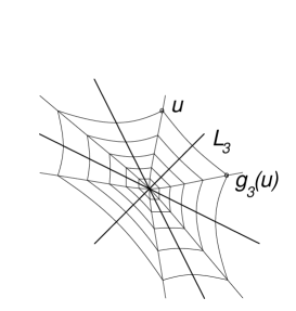
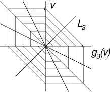
Figure 3: Briançon’s hexagons and their inverse images under the diffeomorphism $\psi$ with $u=\psi(v)$.

Then there is a unique local homeomorphism $\psi:\mathbb{R}^{2},0\to\mathbb{R}^{2},0$ such that
1) $\psi(0,1)=u$,
2) $\psi(1,0)=g_{3}(u)$,
3) it maps the foliations $p=const$, $p+q=const$ and $q=const$ to the foliations $\mathcal{F}_{1}$, $\mathcal{F}_{2}$ and $\mathcal{F}_{3}$ respectively. (See Fig. 3). In fact, the points $u$ and $g_{3}(u)$ lies on the same curve of the foliation $\mathcal{F}_{2}$ since the involution $g_{3}$ is a symmetry of $\mathcal{F}_{2}$. Further, there is a unique diffeomorphism, mapping the triangle $(0,0),(0,1),(1,0)$ to the ”triangle” $(0,0),u,g_{3}(u)$ formed by the curves of the foliations $\mathcal{F}_{1}$, $\mathcal{F}_{2}$ and $\mathcal{F}_{3}$ (see [5] p.15). This map is uniquely extended to the whole hexagon. Moreover, the constructed homeomorphism $\psi$ is equivariant with respect to the action of $\mathbb{D}_{3}$ defined above. The map $\psi$ is smooth (analytic) if the foliations $\mathcal{F}_{1}$,$\mathcal{F}_{2}$,$\mathcal{F}_{3}$ are smooth (analytic). Really, according to [5] p.155, there exists a smooth (analytic) map, taking the foliations $p=const$, $p+q=const$ and $q=const$ to $\mathcal{F}_{1}$, $\mathcal{F}_{2}$ and $\mathcal{F}_{3}$ respectively, and this map is uniquely defined by specifying the inverse image of $u$. Thus this map should coincide with the above homeomorphism $\psi$.

Now consider the map:

$$\pi\circ f\circ\psi:\mathbb{R}^{2},0\to R^{2},0,\ \ (P,Q)\mapsto(A,B)=\pi(f(\psi(P,Q))).$$

In coordinates it reads as

$$A=\alpha(P,Q),\ B=\beta(P,Q).$$

Observe that the above map is symmetric with respect to the action of $\mathbb{D}_{3}$. Then by the results on smooth functions, invariant with respect to finite group action, the functions $\alpha$ and $\beta$ must depend only on the basic invariants of the above $\mathbb{D}_{3}$ group action (see [17]) and [25]):

$$A=\tilde{\alpha}(X,Y),\ B=\tilde{\beta}(X,Y),$$

where

$$X=-P^{2}-PQ-Q^{2},\ \ Y=PQ(P+Q).$$ (38)

We claim that $\tilde{\alpha},\tilde{\beta}$ are the components of the searched for diffeomorphism $\varphi$. To prove that consider the following commutative diagram:

$$\begin{array}[]{ccc}\mathbb{R}^{2},0&\stackrel{{\scriptstyle\psi}}{{\longrightarrow}}&\mathbb{R}^{2},0\\ \downarrow V&&\downarrow\pi\circ f\\ \mathbb{R}^{2},0&\stackrel{{\scriptstyle\varphi}}{{\longrightarrow}}&\mathbb{R}^{2},0\\ \end{array}$$ (39)

where $V$ is Vieta’s map (38). Applying the same results on symmetric functions to $\theta:=V\circ\psi^{-1}$ we see that the differentiable map $\theta$ is inverse to $\varphi$ inside the ”cusped” domain where our ODE has 3 distinct real solutions. This completes the proof in the real analytic case. For the smooth case we apply $\varphi$ and for the reduced equation we consider the first integral of the direction field $\tau$ that coincides with $p$ on the part $M_{3}$ of $M$ that is projected to the domain with three real roots. Further, it is easy to construct through homotopy the $\pi$-lowerable diffeomorphism $\varphi^{\prime}$ of $M$ that is identity on $M_{3}$ and moves the integral curves of $\tau$ to that of (34). The searched for diffeomorphism is $\varphi^{\prime}\circ\varphi$

$\Box$

3.2 The case of non-Legendrian criminant

Theorem 7

If the following conditions hold for implicit ODE (1) at a point $m=(x_{0},y_{0},p_{0})\in M$:
1) ODE (1) has a hexagonal 3-web of solutions,
2) $p_{0}$ is the triple root of (1) at $\pi(m)=(x_{0},y_{0})$,
3) the criminant $C$ is transverse to the contact plane field in some punctured neighborhood of $m$ and ${\rm rank}((x,y,p)\mapsto(F,F_{p}))|_{C}=2$,
then it is locally equivalent to

$$P^{3}+2PX+Y=0,$$ (40)

within the domain, where (40) has three real roots, if $F$ is smooth,
and in some neighborhood of $(0,0)$, if $F$ is real analytic.

Proof: We follow the proof scheme for Theorem 6. Namely we consider the pull-back of the form $dy-pdx$ to $\mathbb{R}^{2},0$ by the Vieta map $\pi\circ f$, where $f$ is defined by (36), duplicate this pull-back form by linear involutions (37) and find a local diffeomorphism of $\mathbb{R}^{2},0$ matching ”lifted” 3-web of our equation and that of (40). The difference to the previous case of Legendrian criminant is that now the web is singular; each foliation $\mathcal{F}_{i}$ has a saddle singular point at $f^{-1}(m)$. Therefore the classical results on hexagonal 3-web are not of much use to find the diffeomorphism ”upstairs”. We construct it through a homotopy of the first integrals of the corresponding foliations.

$\bullet$Differential forms of the foliations.
By Lemma 2 equation (1) is equivalent to (32) with $A(0,0)=B(0,0)=B_{x}(0,0)=0$, $\left.\frac{\partial(A,B)}{\partial(x,y)}\right|_{0}\neq 0$ and

$$A_{x}(0,0)\neq 0,\ \ B_{y}(0,0)\neq 0.$$

Thus the tangent plane $T_{m}M$ to the surface $M$ at $m=(0,0,0)$ is the plane $y=0$ and the tangent line to the discriminant curve at $(0,0)$ is $y=0$. Therefore one can choose $p,A$ as local coordinates on the surface $M,m$ and $A,B$ as local coordinates on $\mathbb{R}^{2},0$. Thus $x=X(A,B),\ \ y=Y(A,B),$ where $A=-p^{2}-q^{2}-pq$ and $p,q,r=-p-q$ are roots of (32). As easily follows from Theorem 5, the kernel of the pull-back form $\pi^{*}(dy-pdx)$ is tangent to the curve $D$ defined by (35). That means that the kernel of the form

$$f^{*}(\pi^{*}(dy-pdx))=(2p+q)(-Y_{A}+pX_{A}+qY_{B}-pqX_{B})dp+(2q+p)(-Y_{A}+p(X_{A}+Y_{B})-p^{2}X_{b})dq$$

is tangent to the line $L_{1}:=\{(p,q):\ p+2q=0\}.$ Writing the above form as $\omega_{1}:=(2p+q)P(p,q)dp+(2q+p)Q(p,q)dq$ with suitable $P,Q$ and passing to the coordinates $q,\ s=2q+p$ one gets

$$\omega_{1}=(2s-3q)Pds+(sQ-2(2s-3q)P)dq$$

hence the tangency condition implies $P|_{s=0}=0$. By the Hadamard lemma $P=s\tilde{P}$ hence one obtains

$$\omega_{1}=s\{(2s-3q)\tilde{P}ds+(Q-2(2s-3q)\tilde{P})dq\}.$$

Now consider the expression for $P=-Y_{A}+(s-2q)X_{A}+qY_{B}-(s-2q)qX_{B}$. One has $Y_{A}=0,$ $X_{A}\neq 0$ from $A_{x}B_{y}\neq 0$, $B_{x}=0$. Since $A$ is quadratic and $B$ is cubic in $p,q$, the term $Y_{A}$ does not have linear terms in $p,q$. This implies $\tilde{P}(0,0)\neq 0$. Using again the condition on $L_{1}$ one obtains

$$Q-2(2s-3q)\tilde{P}=s\tilde{Q}.$$

Let as normalize the forms vanishing each on its own family of solutions to satisfy $\sigma_{1}+\sigma_{2}+\sigma_{3}=0$:

$$\sigma_{1}=(q-r)(dy-pdx),\ \ \sigma_{2}=(r-p)(dy-qdx),\ \ \sigma_{3}=(p-q)(dy-rdx).$$ (41)

As shown above the pull-back of $\sigma_{1}$ is

$$\tilde{\sigma_{1}}=(2q+p)^{2}\{(2p+q)\tilde{P}dp+(2(2p+q)\tilde{P}+(2q+p)\tilde{Q})dq\}$$ (42)

$\bullet$Connection form.
Following [6] consider the area form

$$\Omega:=\tilde{\sigma_{1}}\wedge\tilde{\sigma_{2}}=\tilde{\sigma_{2}}\wedge\tilde{\sigma_{3}}=\tilde{\sigma_{3}}\wedge\tilde{\sigma_{1}}=(Y_{A}X_{B}-Y_{B}X_{A})(p-q)^{2}(2p+q)^{2}(2q+p)^{2}dp\wedge dq$$

and the connection form

$$\gamma:=h_{2}\tilde{\sigma_{1}}-h_{1}\tilde{\sigma_{2}}=h_{3}\tilde{\sigma_{2}}-h_{2}\tilde{\sigma_{3}}=h_{1}\tilde{\sigma_{3}}-h_{3}\tilde{\sigma_{1}},$$

where $h_{i}$ are defined by

$$d\tilde{\sigma_{i}}=h_{i}\Omega.$$

Using (42) on obtains by direct calculation that

$$h_{1}=\frac{R_{1}}{(2p+q)^{2}(p-q)^{2}},$$

where $R_{1}$ is a smooth function of $p,q$. Applying the cyclic permutation $p\rightarrow q,\ q\rightarrow r,\ r\rightarrow p$, one gets: $\tilde{\sigma_{2}}=(2p+q)^{2}\bar{\sigma_{2}}$, $h_{2}=\frac{R_{2}}{(2q+p)^{2}(p-q)^{2}},$ where $R_{2}$ and $\bar{\sigma_{2}}$ are smooth. Therefore

$$\gamma=\frac{\bar{\gamma}}{(p-q)^{2}},$$

with a smooth form $\bar{\gamma}$. Observe that the connection form $\gamma$ is symmetric with respect to the linear transformation group $\mathbb{D}_{3}$, generated by $g_{1},g_{2},g_{3}$. Therefore $\gamma$ is smooth, i.e. $(p-q)^{2}$ divides $\bar{\gamma}$.

$\bullet$Existence of first integrals.
As the web is hexagonal the connection form $\gamma$ is closed. Therefore there exists a unique $\mathbb{D}_{3}$-symmetric function $\mu$, satisfying

$$d\mu=\mu\gamma,\ \ \mu(0,0)=1.$$

Further, the forms $\mu\tilde{\sigma_{i}}$ are also closed, thus defying functions $u_{i}$ by

$$d(u_{i})=\mu\tilde{\sigma_{i}},\ \ u_{i}(0,0)=0,$$

satisfying the following equation, which is equivalent to the hexagonality of the web:

$$u_{1}+u_{2}+u_{3}\equiv 0.$$ (43)

Observe that the function $u_{1}$ is skew-symmetric with respect to $g_{1}$:

$$g_{1}^{*}(u_{1})=-u_{1}.$$ (44)

This follows from (41) and from the invariance of $\mu$. Applying Hadamard’s trick one estimates $u_{1}$ as follows:

$$u_{1}(p,q)=\int_{0}^{1}\frac{d}{dt}u_{1}(tp,tq)dt=\int_{0}^{1}\left(p\frac{\partial}{\partial p}u_{1}(tp,tq)+q\frac{\partial}{\partial q}u_{1}(tp,tq)\right)dt=$$

$$=(2q+p)^{2}\int_{0}^{1}\mu(tp,tq)\left(p(2p+q)\tilde{P}(tp,tq)+q(2(2p+q)\tilde{P}(tp,tq)+(2q+p)\tilde{Q}(tp,tq))\right)t^{3}dt.$$

Collecting similar terms, using $\tilde{P}(0,0)\neq 0$ and integrating one has

$$u_{1}(p,q)=(2q+p)^{3}((2p+q)\hat{P}(p,q)+q\hat{Q}(p,q)),\ \ {\rm where}\ \ \hat{P}(0,0)\neq 0.$$ (45)

$\bullet$Properties of the first integrals.
It follows from Malgrange’s Preparation Theorem that any smooth function $F$ of $(p,q)$ can be represented in the form

$$F(p,q)=F_{0}(A,B)+pF_{1}(A,B)+qF_{2}(A,B)+pqF_{3}(A,B)+q^{2}F_{4}(A,B)+pq^{2}F_{5}(A,B),$$ (46)

with smooth functions $F_{i}$. In fact, the identities $p^{2}=-pq-q^{2}-A$, $p^{3}=-pA-B$, $p^{2}q=-pq^{2}+B$, $q^{3}=-qA-B$ imply $\langle p,q\rangle^{4}\subset\langle A,B\rangle$ and $\mathcal{E}(\mathbb{R}^{2})/\langle A,B\rangle=\mathbb{R}\{1,p,q,pq,q^{2},pq^{2}\}.$ (Here $\mathcal{E}(\mathbb{R}^{2})$ is the local algebra of smooth map germs at $(0,0)$, $\langle p,q\rangle$ its maximal ideal, generated by the coordinate functions $p$ and $q$, $A:(p,q)\mapsto-p^{2}-pq-q^{2}$, $B:(p,q)\mapsto p^{2}q+q^{2}p$, and $\mathbb{R}\{1,p,q,pq,q^{2},pq^{2}\}$ is the real vector subspace of $\mathcal{E}(\mathbb{R}^{2})$, spanned by $1,p,q,pq,q^{2},pq^{2}$.) Moreover, inside the ”cusped” domain with 3 real distinct solutions of our ODE the functions $F_{i}$ are uniquely determined by $F$. For $F=u_{1}$ property (44) implies $F_{4}=-F_{3},$ $F_{2}=2F_{1}-AF_{5}$, $F_{0}=-AF_{3}-BF_{5}/2$. Applying $-g_{2}^{*}$ and $-g_{3}^{*}$ to $u_{1}$ one gets the other two first integrals $u_{2}$ and $u_{3}$, whose representations in form (46) are easily read from the representation of $u_{1}$. Now identity (43) implies $F_{5}=0$. Thus

$$u_{1}(p,q)=(2q+p)(F_{1}(A,B)+pF_{3}(A,B)).$$ (47)

Using (45) one can write

$$F_{1}(A,B)+pF_{3}(A,B)=(2q+p)^{2}G(p,q).$$

Representing the function $G$ as

$$G(p,q)=G_{0}(A,B)+pG_{1}(A,B)+qG_{2}(A,B)+pqG_{3}(A,B)+q^{2}G_{4}(A,B)+pq^{2}G_{5}(A,B)$$

and substituting this representation into the above equation, one obtains

$$G(p,q)=\frac{4}{3}AG_{4}(A,B)+pG_{1}(A,B)+pqG_{4}(A,B)+q^{2}G_{4}(A,B).$$ (48)

$\bullet$Equivariant homotopy.
For equation (40) the first integral $u_{1}$ is $u_{0}(p,q):=p(2q+p)^{3}$. Let us scale $u_{1}$ so that $\hat{P}(0,0)=\frac{1}{2}$ in (45). We claim that the family of functions

$$u_{t}(p,q):=u_{0}(p,q)+t(u_{1}(p,q)-u_{0}(p,q))$$

is equivariantly $\mathcal{R}$-trivial, i.e. for any $t\in[0,1]$ there is a diffeomorphism $\psi_{t}$, equivariant with respect to above $\mathbb{D}_{3}$ group action, such that

$$u_{t}\circ\psi_{t}=u_{0}.$$

To prove this it is enough to find $\mathbb{D}_{3}$-equivariant vector field $\xi(p,q,t)\partial_{p}+\eta(p,q,t)\partial_{q}$ satisfying the following homotopy equation:

$$\xi(p,q,t)\frac{\partial u_{t}(p,q)}{\partial p}+\eta(p,q,t)\frac{\partial u_{t}(p,q)}{\partial q}+\frac{\partial u_{t}(p,q)}{\partial t}=0,\ \ \xi(0,0,t)=\eta(0,0,t)=0.$$

A general form of a $\mathbb{D}_{3}$-equivariant vector field is given by

$$\xi=p\alpha(A,B)+\left(\frac{A}{3}+pq+q^{2}\right)\beta(A,B),\ \ \eta=q\alpha(A,B)-\left(\frac{2}{3}A+q^{2}\right)\beta(A,B),$$ (49)

(see [4] or derive it from the representations of $\xi,\eta$ in form (46)). Observe that the difference $(u_{1}(p,q)-u_{0}(p,q))=\frac{\partial u_{t}(p,q)}{\partial t}$ also has form (48):

$$u_{1}(p,q)-u_{0}(p,q)=\frac{4}{3}AL(A,B)+pK(A,B)+pqL(A,B)+q^{2}L(A,B)$$

with $K(0,0)=0$ due to the chosen scaling of $u_{1}$. Solving the homotopy equation yields the following expressions for $\alpha$ and $\beta$:

$$\alpha=\frac{6K+(6K^{2}+2A^{2}(K_{B}L-KL_{B})+9B(KL_{A}-K_{A}L)+10AL^{2})t}{M},$$

$$\beta=\frac{-12L+(6A(KL_{A}-K_{A}L)+9B(KL_{B}-K_{B}L)+3KL)t}{M},$$

where

$$M=-24+[-48K-12AK_{A}-18B(K_{B}+2L_{A})+8A^{2}L_{B}]t+$$

$$+[-24K^{2}-2A(6KK_{A}+25L^{2})+3B(15K_{A}L-6KK_{B}-12KL_{A})+$$

$$+2A^{2}(4KL_{B}-10LL_{A}-5K_{B}L)-30ABLL_{B}+(27B^{2}+4A^{3})(K_{A}L_{B}-K_{B}L_{A})]t^{2}.$$

$M$ does not vanish at $(0,0)$ since $K(0,0)=0$. The claim on $\mathcal{R}$-triviality of the family $u_{t}(p,q)$ is proved.

$\bullet$Diffeomorphism.
We have proved that the diffeomorphism

$$\psi:=\psi_{1}$$

maps the fibres of $u_{0}$, i.e. the curves $\{(p,q):u_{0}(p,q)=const\}$ to those of $u_{1}$. Therefore, being equivariant, $\varphi$ maps the foliations $\mathcal{F}_{i}$ of (40) to that of our equation (32). Now diagram (39) defines again the desired diffeomorpfism $\varphi$.                                                                       $\Box$

Remark. The pictures of the $\mathbb{D}_{3}$-symmetric hexagonal 3-web, defined by the solutions of (40) and lifted to the plane $p+q+r=0$, is presented in Fig. 4 on the left. It consists of 3 foliations, one of them is shown in Fig. 4 in the center. On the right is the fundamental domain of $\mathbb{D}_{3}$-group (compare with Fig. 1 on the right). The flower-like form on the left suggests that the web is actually symmetric with respect to the symmetry group $\mathbb{D}_{6}$ of regular hexagon. In fact, it is the case since the fibers of the first integrals are permuted by the following symmetry $g_{4}:\mathbb{R}^{2}\to\mathbb{R}^{2},\ (p,q)\mapsto(-p,-q)$.

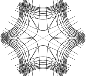
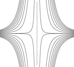
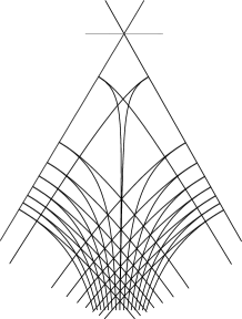
Figure 4: $\mathbb{D}_{3}$-symmetric hexagonal web of 3 foliations with saddle singularities (left), one of the foliations (center) and the fundamental domain of $\mathbb{D}_{3}$ (right).

4 Proof of the classification theorem

Now we can prove Theorem 1. If a point $m=(x_{0},y_{0},p_{0})\in M$ is regular then our equation is locally equivalent to (12v) by definition. If $p_{0}$ is a double root then the regularity condition (4) implies that $m$ is a fold point of the projection $\pi$. Futher Corollary 1 implies that the criminant is either Legendrian or transverse to the contact plane field in some neighborhood of $m$. Thus by Theorems 3 and 5 the equation is locally equivalent either to (12iii) or to (12iv). Finally if $p_{0}$ is a triple root and the criminant is either Legendrian or transverse to the contact plane field in some punctured neighborhood of $m$ then by Theorems 6 and 7 the equation is locally equivalent either to (12i) or to (12ii). To complete the proof we show that Legendrian and non-Legendrian parts of the criminant can not be glued together at a cusp point. By Lemma 2 our equation is equivalent to (32) with $(x_{0},y_{0},p_{0})=(0,0,0)$, $B_{x}(0,0)=0$. Suppose the criminant is transverse to the contact plane field for $p>0$ and Legemdrian for $p\leq 0$. For any point $m^{\prime}\neq m$ with $p>0$ on the curve $D$ defined by (35) the direction field $\tau$ is tangent to $D$ by theorem 5. This condition reads as

$$\left(\left.d(A+\frac{3}{4}p^{2})\wedge(dy-pdx)\right)\right|_{D}=0.$$

In coordinates $p,x$ on $M$ it can be rewritten as follows

$$\left(\left.(dA+\frac{3}{2}pdp)\wedge((3p^{2}+A)dp+(B_{x}+(A_{x}+B_{y})p+A_{y}p^{2})dx)\right)\right|_{D}=0.$$

Substituting $A=-\frac{3}{4}p^{2}$ and

$$dA=A_{x}dx+A_{y}dy=A_{x}dx-\frac{A_{y}}{B_{y}+A_{y}p}((3p^{2}+A)dp+(B_{x}+A_{x}p)dx)$$

into this equation one gets

$$\left.\frac{3}{2}p^{2}(A_{x}B_{y}+A_{y}(A_{x}+B_{y})p+A_{y}^{2}p^{2})-p(B_{x}+(A_{x}+B_{y})p+A_{y}p^{2})(B_{y}+A_{y}p)\right|_{D}=0.$$

Parameterizing the curve $D$ by $p$, expanding the above equation by Tailor formula at $p=0$ and equating the coefficient by $p^{2}$ to $0$ one obtains

$$\left.B_{y}(\frac{3}{2}A_{x}-(A_{x}+B_{y}))\right|_{x=y=0}=0,$$

which implies

$$2B_{y}(0,0)-A_{x}(0,0)=0,$$

since $B_{y}(0,0)\neq 0$. (We have used the Taylor formula $B_{x}=B_{xA}A+B_{xB}B+...=B_{xA}(-3/4p^{2})+B_{xB}(-1/4p^{3})+...$.)

On the other hand, for any point $m^{\prime}\neq m$ with $p\leq 0$ the contact form vanishes on the criminant:

$$\left.dy-pdx\right|_{C}=0.$$

In coordinates $p,x$ on $M$ it can be rewritten as follows

$$\left.(B_{x}+(A_{x}+B_{y})p+A_{y}p^{2})\right|_{C}=0.$$

Now the Tailor expansion at $p=0$ for $C$ parameterized by p gives $A_{x}+B_{y}=0$ ($B_{x}$ does not have linear in $p$ terms). Comparing with the condition above on the non-Legendrian part one gets $A_{x}(0,0)=0$ and therefore $B_{y}(0,0)=0$ which contradicts Lemma 2.

$\Box$

Remark. Unfortunately, the annoying stipulation in Theorem 1 for the smooth case (12i) can not be omitted to guarantee the existence of the diffeomorphism $\varphi$ reducing ODE under consideration to (12i) in some neighborhood of $m$ if one stays within the framework of geometric Definition 1. A necessary condition for that is the existence of the first integral of $\tau$ in the form $f(p,x)^{2}g(p,q)^{3}=\tilde{\varphi}^{*}(p^{2}(x+3p^{2}/8)^{3})$. Here $\tilde{\varphi}$ is the lift to $M$ of the searched for diffeomorphism and $p^{2}(x+3p^{2}/8)^{3}$ is the first integral of $\tau$ for (12i). It is not hard to find a counterexample which does not have such an integral in the form $f(p,x)^{2}g(p,q)^{3}$ with not vanishing $df,dg$ at $(0,0)$. This drawback is repaired as follows. One replace definition 1 with a less geometric one.

Definition 2

We say that implicit ODE (32) has a hexagonal 3-web of solutions if $A,B$ satisfy PDE (33) and the domain, where (32) has 3 real roots $p_{1},p_{2},p_{3}$ is not empty.

The proof of Theorem 7 is easily modified for the case of one real root $p_{1}=p$ and two complex conjugated roots $p_{2,3}=-p/2\pm iz$. The form $\sigma_{1}$ turns out to be pure imaginary but the connection form $\gamma$ is real. All analytical properties being the same, one finds the diffeomorpfism $\varphi$ similarly through homotopy.

5 Concluding remarks

$\bullet$ Symmetries of the normal forms. The solutions of equation (12v) are the lines $dx=0$, $dy=0$ and $dx+dy=0$. The symmetry group of (12v) is generated by the following operators:

$$X_{1}=\partial_{x},\ \ X_{2}=\partial_{y},\ \ X_{3}=x\partial_{x}+y\partial_{y}.$$

Thus the symmetry pseudogroup of a cubic implicit ODE with hexagonal 3-web of solutions is at most 3-dimensional. In a neighborhood of the projection of a regular point $m\in M$ it is generated by the above three operators $X_{i}$ in suitable coordinates. The coordinate change becomes singular on the discriminant curve and not all symmetry operators ”survive” at $\pi(m)\in\Delta$. The symmetry pseudogroups of equations (12iii) and (12iv) at a fold point are generated by

$$Y_{1}=x\partial_{x}+2y\partial_{y},\ \ Y_{2}=\partial_{x}$$

and

$$Y_{1}=2x\partial_{x}+3y\partial_{y},\ \ Y_{2}=\partial_{y},$$

respectively. This easily follows from Propositions 2 and 3. Irreducible equations (12i) and (12ii) have only one-dimensional symmetry pseudogroup at $(0,0)$:

$$Z=2x\partial_{x}+3y\partial_{y}.$$

$\bullet$ Analytic properties. All equations in the given normal forms are integrable in elementary functions.

$\bullet$ Implicit cubic ODEs with singular surfaces $M$. Suppose our cubic ODE factors out to 3 linear in $p$ terms $p-f_{i}(x,y)$ such that 2 of 3 smooth surfaces $M_{i}:=\{(x,y,p):p=f_{i}(x,y)\}$ intersect transversally along a non-singular curve, the solutions of these 2 factors being transverse to the curve projection into the plane. Then one can bring these two factors to the forms $p=0$ and $p=2x$ respectively. The symmetry pseudogroup of the quadratic ODE $p(p-2x)=0$ is $\tilde{y}=F(y),\ \ \tilde{x}=\sqrt{F(y)-F(y-x^{2})}.$ If our cubic equation has a hexagonal 3-web of solutions then its third factor is generated by the vector field $(\alpha(y-x^{2})+\beta(y))\partial x+2x\beta(y)\partial_{y}$. As the functions $\alpha,\beta$ are arbitrary we can hope to ”kill” only one of them by the above mentioned symmetry. Thus a general classification of all cubic ODEs will have functional moduli even if one impose hexagonality condition. (Note that if the third family of solutions in the example is transverse to the first two, we have $\beta=-\alpha$ and one gets a finite classification list.)

$\bullet$ Other examples. The proof of Theorem 7 suggests the following procedure to generate cubic ODEs with a hexagonal 3-web of solutions: start with a function $F(p,q)$ written in form (46) with $A=p^{2}+pq+q^{2},$ $B=pq(p+q)$, define $G(p,q):=F(q,-p-q)$, $H(p,q):=F(-p-q,p)$ and solve the following equations for $F_{i}$:

$$g_{3}^{*}(F)=\pm F,\ \ F+G+H\equiv 0.$$ (50)

This gives four of six coefficients $F_{i}$ as linear combinations of the remaining two ”free” functions of $A,B$. Then the fibers of $F,G,H$ define a hexagonal 3-web, symmetric with respect to $\mathbb{D}_{3}$-group action, generated by the involutions $g_{1},g_{2},g_{3}$. The image of this web under Vieta map $(p,q)\mapsto(p^{2}+pq+q^{2},pq(p+q))$ is a hexagonal 3-web of solutions of some implicit cubic ODE. For example, starting with $F=p-q$ one gets the following equation:

$$yp^{3}-\frac{2}{3}x^{2}p^{2}+xyp+\frac{1}{27}(2x^{3}-27y^{2})=0.$$

The solution 3-web of this equation is dual to that of (12i) (see [24]). Its surface $M$ is not smooth at $(0,0,0)$. Note that one can also start with $F$ such that the ”free” coefficients $F_{i}$ have poles at $0$. This approach linearizes the problem of finding local solutions of nonlinear PDE (33). On the space of functions $F$ satisfying (50) acts the pseudogroup of $\mathbb{D}_{3}$-equivariant transformations with the tangent space generated by vector fields defined by (49). General classification of such functions with this equivalence group seems rather unpromising since the orbit codimension quickly becomes infinite.

6 Acknowledgements

The author thanks L.S.Challapa, M.A.S.Ruas, J.H.Rieger for useful discussions. This research was partially supported by DAAD grant 415-br-probral/po-D/04/40407.

References

- [1]
- [2]
- [3] Arnold, V. I.,Geometrical methods in the theory of ordinary differential equations, Grundlehren der Mathematischen Wissenschaften, 250, Springer-Verlag, New York-Berlin, 1983.
- [4] Arnold, V. I., Wave front evolution and equivariant Morse lemma, Comm. Pure Appl. Math. 29 (1976), no. 6, 557–582.
- [5] Blaschke, W., Bol, G., Geometrie der Gewebe, Topologische Fragen der Differentialgeometrie. J. Springer, Berlin, 1938.
- [6] Blaschke, W., Einführung in die Geometrie der Waben, Birkhäuser Verlag, Basel und Stuttgart, 1955.
- [7] Bruce, J. W., A note on first order differential equations of degree greater than one and wavefront evolution, Bull. London Math. Soc. 16 (1984), no. 2, 139–144.
- [8] Bruce, J. W., Tari, F., On binary differential equations, Nonlinearity 8 (1995), no. 2, 255–271.
- [9] Bruce, J. W., Tari, F., Dupin indicatrices and families of curve congruences, Trans. Amer. Math. Soc. 357 (2005), no. 1, 267–285.
- [10] Challapa, L.S., Index of quadratic differential forms, Contemporary Math. 459 (2008), 177–191.
- [11] Dara, L., Singularite’s ge’ne’riques des e’quations diffe’rentielles multiformes. Bol. Soc. Brasil. Mat. 6 (1975), no. 2, 95–128.
- [12] Davydov, A. A., The normal form of a differential equation, that is not solved with respect to the derivative, in the neighborhood of its singular point. Funktsional. Anal. i Prilozhen. 19 (1985), no. 2, 1–10, 96.
- [13] Dubrovin, B., Geometry of 2D topological field theories. Integrable systems and quantum groups, 120–348, Lecture Notes in Math. 1620, Springer, Berlin, 1996.
- [14] Ferapontov, E. V., Systems of three differential equations of hydrodynamic type with a hexagonal -web of characteristics on solutions, Funct. Anal. Appl. 23 (1989), no. 2, 151–153.
- [15] Ferapontov, E. V., Integration of weakly nonlinear semi-Hamiltonian systems of hydrodynamic type by the methods of web theory, (Russian) Mat. Sb. 181 (1990), no. 9, 1220–1235, translation in Math. USSR-Sb. 71 (1992), no. 1, 65–79.
- [16] Ferapontov, E. V., Invariant description of solutions of hydrodynamic-type systems in hodograph space: hydrodynamic surfaces, J. Phys. A 35 (2002), no. 32, 6883–6892.
- [17] Glaeser, G., Fonctions compose’es diffe’rentiables. Ann. of Math. (2) 77 (1963), 193–209.
- [18] Graf, H., Sauer. R., Über dreifache Geradensysteme in der Ebene, welche Dreiecksnetze bilden, Sitzungsb. Math.-Naturw. Abt. (1924), 119 -156.
- [19] Gutierrez, C., Oliveira, R. D. S., Teixeira, M. A., Positive quadratic differential forms: topological equivalence through Newton polyhedra, J. Dyn. Control Syst. 12 (2006), no. 4, 489–516.
- [20] Hayakawa, A., Ishikawa, G., Izumiya, S., Yamaguchi, K., Classification of generic integral diagrams and first order ordinary differential equations. Internat. J. Math. 5 (1994), no. 4, 447–489.
- [21] Mignard, G., Rang et courbure des 3-tissus de , C. R. Acad. Sci. Paris Se’r. I Math. 329 (1999), no. 7, 629–632.
- [22] Nakai, I., Notes on versal deformation of first order PDEs and web structure, J. Differential Equations 118 (1995), no. 2, 253–292.
- [23] Nakai, I., Web geometry and the equivalence problem of the first order partial differential equations, Web theory and related topics, World Sci. Publ., River Edge, NJ, 2001, 150–204.
- [24] Nakai, I., Web Geometry of Solutions of First Order ODEs, Geometry and Foliations 2003, Kyoto, JAPAN, Invited address, (http://gf2003.ms.u-tokyo.ac.jp/abstract/da)
- [25] Schwarz, G. W., Smooth functions invariant under the action of a compact Lie group, Topology 14 (1975), 63–68.
- [26] Thom, R., Sur les e’quations diffe’rentielles multiformes et leurs inte’grales singulie‘res, Bol. Soc. Brasil. Mat. 3 (1972), no. 1, 1–11.