Proton and Neutrino Extragalactic Astronomy

Abstract

The study of extragalactic sources of high energy radiation via the direct measurement of the proton and neutrino fluxes that they are likely to emit is one of the main goals for the future observations of the recently developed air showers detectors and neutrino telescopes. In this work we discuss the relation between the inclusive proton and neutrino signals from the ensemble of all sources in the universe, and the “resolved” signals from the closest and brightest objects. We also compare the sensitivities of proton and neutrino telescopes and comment on the relation between these two new astronomies.

I Introduction

There is a general consensus that the highest energy cosmic rays (CR) are of extragalactic origin because they reach the Earth with an approximately isotropic angular distribution. The magnetic fields of the Milky Way are not sufficiently strong and extended to randomize the directions of particles produced by our own Galaxy, and the this isotropy of these CR is likely to reflect the large scale homogeneity of the universe. It is natural to expect that the extragalactic Ultra High Energy Cosmic Rays (UHECR) are produced in “point–like” astrophysical sources. The identification of these sources, and the clarification of the mechanisms that accelerate particles to these very large energies is clearly one of the crucial goals of the new large acceptance air shower detectors like the Pierre Auger Observatory.

The trajectories of charged particles is bent by the presence of astrophysical magnetic fields, however at sufficiently large rigidity $E/Z$ (with $Z$ the particle electric charge) the magnetic deviations should become sufficiently small to allow the direct imaging of sources with cosmic rays. Unfortunately the intensity and structure of the intergalactic magnetic field are very poorly known, and therefore the region (in source distance and particle energy) where CR astronomy is possible remains very uncertain. It is possible (and there are observational hints) that the CR above $E\gtrsim{\rm few}\times 10^{19}$ eV are already propagating in quasi–linear mode for source distances of order 100 Mpc or more, however the identification of the sources remains difficult because of the very small number of events available, with most of the sources contributing with not more than a single event.

The analysis of the “clustering” of the observed events can give information about the luminosity of the individual sources. After the data of AGASA Hayashida:1996bc ; Takeda:1999sg gave hints of possible clustering. this question has received a significant amount of attention Uchihori:1999gu ; Dubovsky:2000gv ; Sommers:2008ji . In this work we want to make a more quantitative and detailed study on how to interpret the results on the clustering.

The nature of the particles in the UHECR remains a central open questions in the field. In this work we will assume that most of these particles are protons. This hypothesis is consistent with the existing data (if one takes into account the systematic uncertainties on the modeling of hadronic showers) and it is also favored in most theoretical models. Here this assumption is also made to allow a detailed quantitative description of particle propagation in intergalactic space, which is essential for the problem we are considering. It is possible and reasonably straightforward to generalize the discussion to the case of nuclei.

All cosmic ray sources are unavoidably also sources of neutrinos Gaisser:1994yf ; Learned:2000sw because some fraction of a population of relativistic hadrons will necessarily interact with ordinary matter or radiation fields targets inside or near their acceleration site creating pions and other weakly decaying particles that can (chain) decay into neutrinos. Viceversa, the emission of neutrinos imply the existence of relativistic hadrons, and therefore the acceleration of cosmic rays. The catalogues of the CR and neutrino sources are in principle identical. In practice the situation could more complicated, because the energy range studied by the CR and neutrino telescopes differ by several orders of magnitude, and the relation between the neutrino and cosmic ray emission from a source can vary significantly depending on the structure of the source, and it is certainly possible to have bright CR sources that emit a relatively small amount of neutrinos, and viceversa. Nonetheless, it is reasonable to expect that the brighest extragalactic sources of both CR and neutrinos will coincide, and it is interesting to discuss in parallel these new astronomies.

Also in the case of neutrinos one can measure an inclusive flux, that sums the contributions from all sources in the universe, while the brightest and most powerful neutrino sources should be identifiable as individual objects. Therefore also for neutrinos the “clustering” of the detected events is a useful method of study. An important advantage is that for neutrinos linear propagation is certain, but one has to deal with the existence of the foreground of atmospheric neutrinos. The theoretical framework needed to discuss the clustering of neutrino events is essentially identical to the one needed for protons. A quantitative difference is that for neutrinos extragalactic space is perfectly transparent, and the inclusive flux receives most of its contribution from very distant and very faint sources, and the fraction of this flux that can be “resolved” in the contribution of identified sources is likely to be small. More that the interpretation of the existing data, the goal of this work is the development of some general analysis instruments that can be used in the study of future, higher statistics results.

This work is organized as follows: in the next section we make a preliminary discussion of the so called “Olbers Paradox”. The discussion of this celebrated puzzle allows to introduce the key concepts needed to compute the signal from the ensemble of all sources in the universe. In section 3 we collect the results on particle propagation in intergalactic space that are needed in the following. Section 4 discusses how the flux received from one astrophysical source depends on its redshift. Section 5 discusses possible forms of the luminosity function of the proton and neutrino sources. Section 6 compute the inclusive particle flux from the combined emission of all sources in the universe. Section 7 discusses what part of the inclusive flux can be resolved in the contribution of individual sources. Section 8 applies these analysis instruments to the interpretation of the recent Auger data. Section 9 discusses extragalactic neutrino astronomy. Section 10 gives some conclusions.

II The “Kepler–Olbers Paradox”

In 1610 Kepler was the first to note that the darkness of the night sky seems to imply that the universe is finite, or at least contains a finite number of stars. This point was later rediscussed by several authors, and is commonly known in the formulation of Henrich Olbers in 1823. The so called “Olbers paradox” is the statement that in an infinite, homogeneous and static universe the surface of the celestial sphere should be infinitely bright. A derivation of this result is elementary. In euclidean space, the relation between the apparent ($\ell$) and absolute ($L$) luminosity of a source placed at a distance $R$ (neglecting photon absorption) is:

$$\ell=\frac{L}{4\,\pi\,R^{2}}$$ (1)

An homogeneous ensemble of identical sources of density $n_{s}$ produces then an inclusive energy flux per unit of solid angle $dF/d\Omega$ that diverges linearly because every spherical layer contained in the interval [$R,R+dR]$ gives an equal contribution:

$$\left.\frac{dF}{d\Omega}\right|_{\rm inclusive}=\frac{1}{4\,\pi}~{}\int_{0}^{\infty}dR~{}(4\,\pi\,n_{s}\;R^{2})~{}\frac{L}{4\,\pi\,R^{2}}=\frac{n_{s}\;L}{4\,\pi}~{}\int_{0}^{\infty}dR~{}1\to\infty$$ (2)

Assuming the same homogeneous distribution of identical sources, one can also consider the number of objects in the sky that have apparent luminosity in the interval $[\ell,\ell+d\ell]$. The distribution $dN_{s}/d\ell$ can be easily calculated as:

$$\frac{dN_{s}}{d\ell}=\frac{dN_{s}}{dR}\;\frac{dR}{d\ell}=4\,\pi~{}n_{s}~{}\left[R^{2}~{}\left|\frac{d\ell}{dR}\right|^{-1}\right]_{R=\sqrt{\frac{L}{4\,\pi}}}=4\,\pi~{}n_{s}~{}\left(\frac{L}{4\,\pi}\right)^{3/2}~{}\frac{\ell^{-5/2}}{2}~{},$$ (3)

a result that is also often stated in its integral form:

$$N_{s}(\geq\ell_{\rm min})=\int_{\rm\ell_{\rm min}}^{\infty}d\ell~{}\frac{dN_{s}}{d\ell}=n_{s}~{}\frac{4\pi}{3}~{}\left(\frac{L}{4\,\pi\;\ell_{\rm min}}\right)^{3/2}$$ (4)

that has the obvious geometrical meaning of the number of sources contained in a sphere of radius $R_{\ell_{\rm min}}=\sqrt{L/(4\pi\ell_{\rm min})}$. The infinite brightness of the sky is due to the “exploding” number of very faint sources. In fact for $\ell_{\rm min}\to 0$ the number of observed sources diverges $\propto\ell_{\rm min}^{-3/2}$, and correspondingly the integrated energy flux diverges as $\propto\ell_{\rm min}^{-1/2}$.

These elementary results can be also restated in an adimensional form, and in terms of particle fluxes instead of energy fluxes. We consider identical sources emitting $Q$ particles per unit time, and choose a reference length $R_{0}$ (here the choice of $R_{0}$ is completely arbitrary, in the following it will be natural to identify $R_{0}$ with the Hubble length). The particle flux received from a source placed at the distance $R_{0}$ is:

$$\Phi_{0}=\frac{Q}{4\,\pi\;R_{0}^{2}}=\frac{L}{4\,\pi\;\langle E\rangle~{}R_{0}^{2}}$$ (5)

Using the notation: $R=R_{0}\;z$ and $\Phi=\Phi_{0}\;x$ one can rewrite equations (1) and (3) in the equivalent adimensional form:

$$x\equiv\frac{\Phi}{\Phi_{0}}=F(z)=\frac{1}{z^{2}}$$ (6)

$$\frac{dN_{s}}{dx}=4\,\pi\;\left(n_{s}\,R_{0}^{3}\right)~{}G(x)=4\,\pi\;\left(n_{s}\,R_{0}^{3}\right)~{}\frac{x^{-5/2}}{2}$$ (7)

In equations (6) and (7) we have introduced the two functions $F(z)$ and $G(x)$. The function $F(z)=z^{-2}$ can be called the “dimming function”, and describes how the flux from a source decreases as its distance increases. The function $G(x)=x^{-5/2}/2$ can be called the “flux distribution function” and describes how the number of observable sources depends on the size of their flux.

Summing over all sources, the inclusive flux per unit solid angle (as well as the inclusive energy flux) diverges; however it still formally possible to write an expression for the inclusive flux as an integral over the scaled distance $z$:

$$\Phi_{\rm incl} = \frac{R_{0}}{4\,\pi}~{}\left(n_{s}\,Q\right)~{}\int_{0}^{\infty}dz~{}K(z)=\frac{R_{0}}{4\,\pi}~{}\left(n_{s}\,Q\right)~{}\int_{0}^{\infty}dz~{}1\to\infty$$ (8)

The function $K(z)=1$ can be called the “Kepler–Olbers function”, and gives the contribution of the spherical shell between (scaled) distance $z$ and $z+dz$ to the inclusive flux. In general there is an integral relation between $K(z)$ and $G(x)$:

$$\int_{0}^{z}~{}dz~{}K(z)=\int_{F(z)}^{\infty}dx~{}x~{}G(x)$$ (9)

that is easily understood, noting that both sides of the equation describe the particle flux generated inside a sphere around the observer of (scaled) radius $z$.

It is obvious that the three functions $F(z)$, $G(x)$ and $K(z)$ are related to each other and, given one of the three, the other two can be deduced taking into account the hypothesis of static, euclidean space. For example, if the “dimming function” has the general form $F(z)$ the functions $G(x)$ and $K(z)$ can be calculated as:

$$G(x)=\left[\left(\frac{1}{4\,\pi\;R_{0}^{3}}~{}\frac{dV}{dz}\right)~{}\left|\frac{dF(z)}{dz}\right|^{-1}\right]_{x=F^{-1}(z)}$$ (10)

$$K(z)=\left(\frac{1}{4\,\pi\;R_{0}^{3}}~{}\frac{dV}{dz}\right)~{}F(z)$$ (11)

where $dV/dz=4\pi\;R_{0}^{3}\,z^{2}$ is the volume contained in the spherical shell $[z,z+dz]$. In fact equations (10) and (11) remain true for a realistic cosmological model, replacing the volume element $dV/dz$ with the correct general relativity expression of equation (58).

The “Kepler–Olbers paradox” is “solved”, and we observe a finite energy flux even if our universe is (to a very good approximation) euclidean, (nearly certainly) infinitely large and homogeneous, because the additional condition of a static, unchanging universe is false. The calculation of the inclusive flux from the ensemble of all extra–galactic sources must obviously take into account the expansion of the universe, and the consequent (redshift) energy loss of all particles. In addition the particles can lose energy also for other mechanism that must be taken into account. With the inclusion of the cosmological and energy loss effects the functions $F(z)$, $G(x)$ and $K(z)$ take more complex forms that are different the simple result:

$$F(z)=z^{-2},~{}~{}~{}~{}~{}~{}~{}~{}~{}~{}~{}~{}~{}~{}~{}~{}G(x)=\frac{x^{-5/2}}{2}~{}~{}~{}~{}~{}~{}~{}~{}~{}~{}~{}~{}~{}~{}~{}~{}K(z)=1$$ (12)

that is valid for a static, euclidean space universe, and in the absence of energy losses. The form of the functions $F(z)$, $G(x)$ and $K(z)$ in a realistic cosmological model depend on the particle type, the particle energy and encode also the shape of the emission spectrum (and clearly also the parameters that control the expansion of the universe), however the solution (12) will always emerge as the universal asymptotic form for small redshift ($z\to 0$) and the largest fluxes ($x\to\infty$). The modifications have the consequence that the inclusive particle flux, obtained integrating over all possible sources, remains finite. The relation (9) remains valid also in the limit of $z\to\infty$ (and corresponding $x\to 0$):

$$\int_{0}^{\infty}~{}K(z)=\int_{0}^{\infty}dx~{}x~{}G(x)=\zeta_{\Phi}$$ (13)

The result of the integration in (13) is finite and equal to $\zeta_{\Phi}$. The physical meaning of $\zeta_{\Phi}$ can be understood qualitatively as the equivalent linear size (in units of the Hubble scale length $R_{0}$) of the universe that contributes to the flux $\Phi$, or equivalently as the effective number of Hubble times ($t_{0}=R_{0}/c$) that contribute to the flux injection.

III Particle Propagation

III.1 Energy Losses

In this work we will describe the energy losses of neutrinos and protons propagating in extra–galactic space as a continuous deterministic process described by the function $dE/dt(E,z)$ that depends on the particle energy and on the epoch $z$. The assumption of continuous energy loss is essentially exact for neutrinos, that lose energy only because of the redshift effect, but is also a good approximation for protons. Integrating the energy loss over time it is possible to compute the evolution with time (or redshift) of the energy of a particle constructing the function $E_{\rm evolution}(E_{i},z_{i},z_{f})$ that returns the energy at redshift $z_{f}$ of a particle with energy $E_{i}$ at redshift $z_{i}$:

$$E_{f}=E_{\rm evolution}(E_{i},z_{i},z_{f})$$ (14)

Neutrinos, to a very good approximation, only lose energy for the redshift effect, and their energy evolution is:

$$E_{f}=E_{i}~{}\left(\frac{1+z_{i}}{1+z_{f}}\right)$$ (15)

It is particularly important to know the energy at a past epoch $z$ of a particle that is observed “now” with energy $E$. This is a particular case of the general relation (14) and can be indicated (propagating backward in time) as:

$$E_{g}(E,z)=E_{\rm evolution}(E,0,z)$$ (16)

For neutrinos one obviously has:

$$E_{g}(E,z)=E~{}(1+z)$$ (17)

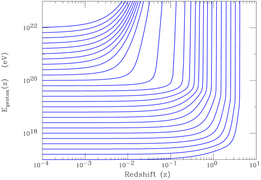
Figure 1: Redshift evolution of the proton energy. The different energies correspond to protons observed at $z=0$ with energy $E_{\rm now}=10^{22-0.1,k}$ eV (with $k=0,$1,$\ldots$,25).

The propagation of protons in intergalactic space has been discussed in several works, after the pioneering work of Greisen, Zatsepin and Kuzmin GZK and is now well understood. Together with the redshift losses one has to include losses due to interactions with the photons of the cosmic microwave background radiation (CMBR). The two important processes are pair production interactions ($p\gamma\to p\,e^{+}e^{-}$) and inelastic hadronic interactions (with the threshold processes $p\gamma\to p\pi^{\circ}$ and $p\gamma\to n\pi^{+}$). The results of a numerical calculation of $E_{g}(E,z)$ for protons are shown in fig. 1. The different curves correspond to the “backward in time” evolution of protons detected “now” with $E$ between $10^{17}$ eV and $10^{22}$ eV. Note that the time evolution of the proton energy is completely independent from the structure and intensity of the magnetic fields, because these fields can only bend the trajectory of charged particles, and the target radiation field is isotropic. Obviously, if the particles do not travel in straight lines, the redshift $z$ has no simple relation with the distance of the particle source, but only describes the time of the particle emission.

Inspection of figure 1 shows that for each observed energy $E$ there is a critical redshift where the energy evolution $E(z)$ “explodes”, starting to grow faster than an exponential. At this critical redshift the universe, filled now with a hotter and denser radiation field, has become opaque to the propagation of the protons.

The form of the redshift evolution of the proton energy suggests the introduction of the concept of a redshift “horizon”. The implicit equation:

$$E_{g}(E,z_{h})=E_{\rm max}$$ (18)

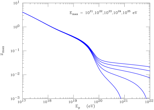
Figure 2: Redshift horizon as a function of the observed proton energy $E$. The different curves are calculated using equation (18) for different values of the maximum acceleration energy $E_{\rm max}$.

(with $E_{\rm max}$ the maximum energy with which protons are produced in their sources) can be used as a definition of the redshift horizon $z_{h}(E,E_{\rm max})$. An illustration of this definition of the redshift horizon is shown in fig. 2. The redshift horizon becomes progressively smaller when the energy $E$ grows. When $E$ becomes a few times 10¹⁹ eV the “shrinking” of the horizon with increasing $E$ accelerates sharply. At this “GZK” energy the protons start interacting with the photons of the background radiation in the present universe, and not only with the higher energy photons of a hotter past. Above this critical “GZK energy” the definition of the horizon with equation (18) strongly depends on the “maximum acceleration energy” (that is not a priori a well defined concept) and therefore loses most of its usefulness. A better definition of the proton horizon will be given later in equation (65).

III.2 Magnetic Deviation

Protons are charged particles, and therefore their trajectories are bent by magnetic fields. Astronomy with protons is therefore possible only in a limited region of source distance and particle energy so that the observed deviations are acceptably small. The size of this region is determined by the strength and structure the astrophysical magnetic fields.

Neglecting the deviations due to to magnetic fields in the vicinity of the source and in the Milky Way halo, the deviation of a charged particle traveling in intergalactic space for a distance $d$ can be described (in the limit of small deviation) with the expression

$$(\delta\theta)^{2}_{\rm extra}\simeq N_{\rm domains}~{}\left(\frac{\lambda_{B}}{r_{L}}\right)^{2}=\left(\frac{d}{\lambda_{B}}\right)~{}\left(\frac{\lambda_{B}}{r_{L}}\right)^{2}=~{}(Z\,e\,B)^{2}\;\lambda_{B}~{}\left(\frac{d}{E^{2}}\right)$$ (19)

where $r_{L}=E/(Z\,e\,B)$ is the Larmor radius, $B$ is the typical value of the extra–galactic magnetic field and $\lambda_{B}$ is its coherence length. In (19) the magnetic deviation is modeled as the incoherent sum of contributions received in “magnetic domains”, where the field has different orientation. In this simple model, the angular deviation accumulated by a proton of energy $E$ from a source at distance $d$ scales $\propto\sqrt{d}/E$, with an absolute value controled by the combination $B\,\sqrt{\lambda_{B}}$.

If we require an image with an angular resolution better that $\delta\theta$, for a given energy $E$ we must limit our observations to distances smaller than an “imaging radius”:

$$R_{\rm imaging}(E,\delta\theta)=\frac{E^{2}\,\delta\theta^{2}}{(Z\,e\,B)^{2}\;\lambda_{B}}$$ (20)

Alternatively to produce an image with resolution $\delta\theta$ of a source at a distance $d$ one must select a threshold energy $E_{\rm imaging}$

$$E_{\rm imaging}(d,\delta\theta)=\frac{\sqrt{d}}{\delta\theta}~{}{(Z\,e\,B)\;\sqrt{\lambda_{B}}}$$ (21)

The combination $B\sqrt{\lambda_{B}}$ is therefore the crucial parameter that controls the perspectives of extragalactic cosmic ray astronomy. The best (and perhaps today the only) way to estimate $B^{2}\,\lambda_{B}$ and determine where CR astronomy is possible is in fact the observation of UHECR and the use of equation (19). At present however the estimate of $B^{2}\,\lambda_{B}$ remains very poorly known.

The recent results of the Auger collaboration Cronin:2007zz ; Abraham:2007si indicates that the directions of the highest energy events ($E\geq 5.6\times 10^{19}$ eV) are correlated with the positions of close AGN’s, selected with a redhift cut $z<0.018$ that corresponds to $d\simeq 75$ Mpc, using a correlation cone of opening angle $\psi\simeq 3.1^{\circ}$. The simplest (“nominal”) interpretation of these results is that the highest energy CR are in fact produced in these AGN (or in sources very strongly correlated in position) and arrive with a magnetic deviation of less than 3.1^∘. This is a remarkable result that, attributing all of the observed deviation to the intergalactic propagation (that is neglecting the contributions of the source envelope and of the Milky Way), allows to set an upper limit on the combination $B^{2}\,\lambda_{B}$ that describes the extragalactic magnetic field:

$$Z^{2}\,B^{2}\;\lambda_{B}\leq 0.15~{}({\rm nGauss})^{2}~{}{\rm Mpc}$$ (22)

Assuming that the particles are protons, this implies the imaging radius:

$$R_{\rm imaging}=210~{}\left(\frac{E}{10^{20}~{}{\rm eV}}\right)^{2}~{}\left(\frac{\delta\theta_{\rm image}}{3^{\circ}}\right)^{2}~{}{\rm Mpc}$$ (23)

This result, if confirmed, indicates that CR astronomy should be able to give important results in the very near future.

The “nominal interpretation” of the Auger results, suffers from several difficulties both internally (see for example the criticism in Gorbunov:2008ef ) and comparing with the observations of other detectors (for the Yakutsk data see Ivanov:2008it for the HiRes data see Abbasi:2008md ). The consensus is that the Auger results do indicate the existence of an anisotropy of the arrival directions of the highest energy cosmic rays, but the origin of the anisotropy has not been established, the significance of the 3.1 degrees of the opening of the correlation cone is therefore ambiguous and the estimates (22) and (23) only tentative.

A remarkable fact of the Auger results is that two of the highest energy events are in correlation (using the 3.1^∘ cone) with the nearby ($d\simeq 3.5$ pc) AGN Cen A. Taking into account the fact that Cen A has been often discussed as one of the most likely sources of UHECR this is a striking result, that suggests that the first extragalactic CR source has in fact already been imaged. There are also indications that Cen A could be the source of a larger number of events with a larger angular spread (see for example the remarks in Wibig:2007pf ; Gorbunov:2008ef ; Stanev:2008sd ). For example a 20 degrees cone around Cen A contains 9 events. Such a large contribution from Cen A could account for a significant fraction of the observed anisotropy effect. These observations could however also a dramatic impact on the estimate of the extragalactic magnetic field, because they suggest a larger deviation ($\delta\theta\sim 10^{\circ}$) for a shorter distance. The estimate for the combination $B^{2}\;\lambda_{B}$ becomes therefore larger by a factor of order 200:

$$Z^{2}\;B^{2}\;\lambda_{B}\simeq 40~{}({\rm nGauss})^{2}~{}{\rm Mpc}$$ (24)

with a correspondingly smaller imaging radius, and significantly restricting the potential of CR astronomy for more distant sources. Additional data should allow to clarify this ambiguous situation. The discrimination between the two estimates (22) and (24) for the parameter that describes the extragalactic magnetic field is obviously crucial for the future of the field.

IV Flux from an individual source

Let us consider a source that emits isotropically particles with the energy spectrum described by the function $q(E)$. The emitted particles travel, at least in good approximation, along geodetic trajectories losing energy continuously. Propagating backward in time, a particle that is observed “now” with energy $E$, at the time that correspond to redshift $z$ had energy $E_{g}(E,z)$.

The flux received from such a source placed at the distance that corresponds to redshift $z$ can be written as:

$$\phi(E,z)=\frac{q(E)}{4\pi\,R_{0}^{2}}~{}F_{\phi}(z,E)$$ (25)

where:

$$R_{0}=\frac{c}{H_{0}}$$ (26)

is the Hubble length, and the adimensional function $F_{\phi}(z,E)$ is given by:

$$F_{\phi}(z,E)=\frac{1}{r^{2}(z)\,(1+z)}~{}\frac{q[E_{g}(E,z)]}{q(E)}~{}\frac{dE_{g}(E,z)}{dE}~{}.$$ (27)

In equation (27) $E_{g}(E,z)$ is the emission energy (at the source) of the particles observed with energy $E$, and $r(z)$ is the (adimensional) comoving coordinate that corresponds to the redshift $z$:

$$r(z)=\int_{0}^{z}\frac{dz^{\prime}}{{\cal H}(z^{\prime})}$$ (28)

with ${\cal H}(z)=H(z)/H_{0}$ the (scaled) Hubble parameter at the epoch of redshift $z$:

$${\cal H}(z)=\sqrt{\Omega_{\rm m}\,(1+z)^{3}+\Omega_{\Lambda}+(1-\Omega_{\rm m}-\Omega_{\Lambda})\,(1+z)^{2}}.$$ (29)

The expansion of the universe, and the redshift dependence of the Hubble constant are determined by the parameters $\Omega_{\rm m}$ and $\Omega_{\Lambda}$.

The “dimming function” $F_{\phi}(z,E)$ describes how the flux of a source weakens, and (in general) has its energy spectrum distorted when the redshift $z$ increases. The function is the generalization of Gauss law ($1/z^{2}$ behaviour) that is valid for static, euclidean space in the absence of energy loss. For small $z$ cosmological and energy loss effects become negligible and the function $F_{\phi}(z,E)$ takes the simple asymptotic form $F_{\phi}(z,E)\to z^{-2}$. The form of the function $F_{\phi}(z,E)$ is determined by the cosmological parameters ($\Omega_{\rm m}$ and $\Omega_{\Lambda}$) and from the shape of the emission spectrum. In principle an unambiguous notation should include these additional dependences: $F_{\phi}(z,E)\to F_{\phi}(z,E;\{q\},\Omega_{\rm m},\Omega_{\Lambda})$. For simplicity, in this work we will leave the dependence on the cosmological parameters and the shape of the emission function implicit.

A relation analogous to (25) can also be written for the integral spectrum:

$$\Phi(E_{\rm min},z)=\frac{Q(E_{\rm min})}{4\pi\,R_{0}^{2}}~{}F_{\Phi}(z,E_{\rm min})$$ (30)

where $Q(E_{\rm min})$ is the integral source emission:

$$Q(E_{\rm min})=\int_{E_{\rm min}}^{\infty}dE~{}q(E)~{}.$$ (31)

The function $F_{\Phi}(z,E)$ (for the integral flux) can be obtained from $F_{\phi}(z,E)$ (for the differential flux) with the integration:

$$F_{\Phi}(z,E_{\rm min})=\frac{1}{Q(E_{\rm min})}~{}\int_{\rm E_{\rm min}}^{\infty}q(E)~{}F_{\phi}(z,E)$$ (32)

For $z\to 0$, the asymptotic behaviour of $F_{\Phi}(z)$ takes again the simple form $z^{-2}$.

For neutrinos, and more in general in all cases when the only significant source of energy loss is the redshift, the energy evolution of a particle has the simple form $E_{g}(E,z)=E\,(1+z)$ the general expression for $F_{\phi}(z,E)$ given in equation (27) can be simplified, obtaining:

$$F_{\phi}(z,E)=\frac{1}{r^{2}(z)}~{}\frac{q[E(1+z)])}{q(E)}$$ (33)

As a consistency check one can observe that a source of such “non interacting” particles of absolute luminosity

$$L=\int_{0}^{\infty}dE~{}E~{}q(E)$$ (34)

placed at a distance $z$, has an apparent luminosity:

$$\ell = \int_{0}^{\infty}dE~{}E~{}\phi(E)=\int_{0}^{\infty}dE~{}E~{}\left(\frac{1}{4\,\pi\,R_{0}^{2}}~{}\frac{1}{r^{2}(z)}~{}q[E(1+z)]\right)$$ (35)

$$= \frac{1}{4\,\pi\,R_{0}^{2}\;r^{2}(z)\,(1+z)^{2}}~{}\left[\int_{0}^{\infty}dE_{0}~{}E_{0}~{}q(E_{0})\right]=\frac{L}{4\,\pi\,d_{L}(z)^{2}}$$

This expression has the well known form $\ell=L/(4\pi\,d_{L}^{2})$, where $d_{L}$ is the “luminosity distance”:

$$d_{L}(z)=R_{0}\;r(z)\,(1+z)~{}.$$ (36)

The “dimming functions” for neutrinos take a very simple form if one makes the assumption that the emission spectrum is un unbroken power law of slope $\alpha$. In this case the functions $F_{\phi}(z)$ and $F_{\Phi}(z)$ become independent from energy, and equal to each other:

$$F_{\phi}(z)=F_{\Phi}(z)=\frac{(1+z)^{-\alpha}}{r^{2}(z)}$$ (37)

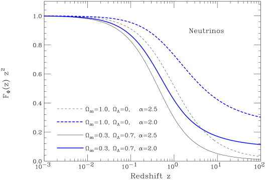
Figure 3: Plot of the function $F_{\phi}(z)=F_{\Phi}(z)$ that gives the redshift dependence of the flux from a $\nu$ source. The source spectrum is a power law of slope $\alpha$. The different curves are calculated for two different choices of the cosmological parameters ($\Omega_{\rm m}$ and $\Omega_{\Lambda}$), and two different slopes ($\alpha=2$ and $\alpha=2.5$).

In case of a power law emission of neutrinos, the spectrum mantains its (featureless) shape even after propagation and energy loss. The function $F_{\phi}(z)$ for neutrinos is shown in figure 3. The function depends on the value of the cosmological parameters $\Omega_{\rm m}$ and $\Omega_{\Lambda}$, and of the value of the slope $\alpha$. One can see that $F_{\phi}(z)$ coincides with the form $z^{-2}$ for $z\lesssim 0.1$, and then begins to fall more rapidly suppressing the flux of very distant sources.

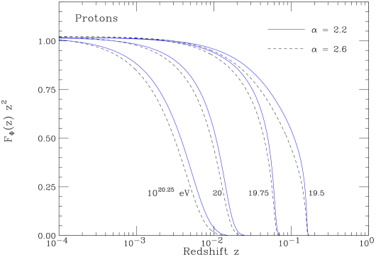
Figure 4: Plot of the function $F_{\Phi}(z,E_{\rm min})$ (in the form $z^{2}\,F_{\Phi}(z)$ versus $z$) for protons. The function $F_{\Phi}(z)$ gives the “dimming” of the integral proton flux above the minimum energy $E_{\rm min}$ with increasing redshift $z$. The solid (dashed) curves are calculated for a proton spectrum slope with slope $\alpha=2.2$ ($\alpha=2.6$), and different values of the threshold energy $E_{\rm min}$.

The “dimming function” for proton sources depends very strongly on the proton energy. Some examples of this behaviour (for the integral flux) are shown in fig. 4 where the redshift dependence of the function $F_{\Phi}(z,E_{\rm min})$ is shown for several value of the threshold energy $E_{\rm min}$, assuming again a power law emission spectrum. One can clearly see that a proton source becomes rapidly unobservable when it becomes more distant than a rather sharply defined “horizon” that shrinks rapidly with energy for $E_{\rm min}\simeq 10^{19}$ to $10^{20}$ eV, and is much smaller that the Hubble length.

V Luminosity Function

In this work we will make the assumption that all astrophysical sources have emission of the same shape and differ only for their absolute luminosity. The idea behind this assumption is that the emission mechanism is likely to be universal, independent from the properties of the individual sources. An example of this situation is the acceleration of cosmic rays near the blast waves of SuperNova (SN) explosions, where it is believed that particles are accelerated with a power law spectrum $\propto E^{-\alpha}$ with a slope $\alpha\simeq 2$ that is essentially independent from the properties of an individual SN (for example the mass and initial velocity of the ejected material), but it is determined only by the (universal) compression factor of the interstellar gas after the passage of a strong shock front.

This assumption of a “universal” spectral shape is of course an hypothesis that could very well be incorrect. This possibility is in fact likely to the UHE proton sources, since it is in fact natural to expect that different sources have different high energy cutoffs, and that these cutoffs are in the energy range where the spectra are measured. After these words of warning, we will anyway make the assumption of a universal shape as it clearly significantly simplifies the discussion, and represents a natural first order approximation.

The luminosity function $dn_{s}/dL(L,z)$ gives the number density (in comoving volume) of sources of luminosity $L$ at the epoch of redshift $z$. The power density ${\cal L}(z)$ of the sources at redshift $z$ is given integrating over all luminosities:

$${\cal L}(z)=\int dL~{}L~{}\frac{dn_{s}}{dL}(L,z)$$ (38)

In this work we will discuss emission spectra that are well represented (at least in the region of interest of the measurements) as simple power laws of constant slope. In this situation however, the source bolometric luminosity is not unambiguously defined because the integral

$$\int_{0}^{\infty}dE~{}E~{}E^{-\alpha}$$

is always divergent (at the upper limit for $\alpha\leq 2$, and at the lower limit for $\alpha\geq 2$). In other words, an unbroken power law emission is impossible, and to estimate the bolometric luminosity of a source it is necessary to specify the range of validity of the power law form, and the behaviour of the spectrum outside this region. This requires the introduction of additional parameters that are not easily constrained, because one observes only a limited range of the spectrum. What is really needed for our purposes is to determine the absolute normalization of the power law spectrum in the energy region of interest. This can be done considering the luminosity in a fixed, relevant energy range. In this work we will use the convention to use the luminosity (or luminosity density) integrated over one energy decade starting from a minimum energy $E_{\rm min}$ that is relevant for the observations

$$L\equiv L_{\rm decade}(E_{\rm min})=\int_{E_{\rm min}}^{10\,E_{\rm min}}dE~{}q(E)$$ (39)

(in the case of $\alpha=2$: the luminosity per energy decade is constant and independent from $E_{\rm min}$): To keep the notation simple in the following the subscript “decade” will be omitted, and the dependence $E_{\rm min}$ (in most cases) will be left implicit. The integral emission of particles above the energy $E_{\rm min}$ is related to this definition of the luminosity by the relation:

$$Q(E_{\rm min},L)=\frac{L~{}\eta}{E_{\rm min}}$$ (40)

where $\eta$ is an adimensional factor that depends on the shape of the spectrum. For a simple power law of slope $\alpha$ one has:

$$\eta=\eta_{\alpha}=\frac{(\alpha-2)}{(\alpha-1)}\left(1-10^{-(\alpha-2)}\right)~{}.$$ (41)

For $\alpha\to 2$ the limit of equation (41) is $\eta_{2}=1/{\ln 10}\simeq 0.434$. The differential and integral spectra for an arbitrary value of the energy (and assuming the validity of the power law behaviour):

$$q(E,L)=\left[\frac{L~{}\eta_{\alpha}\;(\alpha-1)}{E_{\rm min}^{2}}\right]~{}~{}\left(\frac{E}{E_{\rm min}}\right)^{-\alpha}$$ (42)

$$Q(E,L)=\left[\frac{L~{}\eta_{\alpha}}{E_{\rm min}}\right]~{}\left(\frac{E}{E_{\rm min}}\right)^{-\alpha+1}$$ (43)

The simplest hypothesis for the luminosity function is to assume that all sources are identical with luminosity $L_{0}$:

$$\frac{dn_{s}}{dL}=\delta[L-L_{0}]$$ (44)

This is nearly certainly incorrect. As an example, the luminosity function of AGN in the hard $X$–ray band ([10,20] KeV) has been fitted by Ueda ueda with the functional form:

$$\frac{dn_{s}}{dL}(L)=\frac{n_{0}}{L_{c}}~{}\left(\frac{L_{c}}{L}\right)~{}\left[\left(\frac{L}{L_{c}}\right)^{0.86}+\left(\frac{L}{L_{c}}\right)^{2.23}\right]^{-1}$$ (45)

with $L_{c}\simeq 10^{43.94}$ erg/s. This shape provides a good fit for all luminosities $L_{x}\in[10^{41.5},10^{46.5}]$ erg/s, in a broad range that extends for 5 orders of magnitude. In the following we will use expression (45) (shown in figure 5) as a “template” (with two free parameters $n_{0}$ and $L_{c}$, that in principle can also be redshift dependent) to build examples of the luminosity functions for the (yet undiscovered) proton and neutrino extragalactic sources.

Note that the integration of the expression (45) for the luminosity function diverges at the lower limit (corresponding to a divergent number of faint sources) while the power density remains finite. This fact illustrates the point that the concept of “total number of sources” should be treated with caution, because the existence of a large number of weak sources is difficult to establish (or refute). In the following we will use the form of the luminosity distribution (45) assuming also a low luminosity sharp cutoff:

$$L\geq 3\times 10^{-3}\;L_{c}$$ (46)

In this work we will use as the “characteristic” value of the source luminosity the median luminosity $L_{0}$ of the sources at redshift $z=0$, defined as the solution of the equation

$$\int_{0}^{L_{0}}dL~{}L~{}\frac{dn_{s}}{dL}(L,0)=\int^{\infty}_{L_{0}}dL~{}L~{}\frac{dn_{s}}{dL}(L,0)~{}.$$ (47)

Half of the power density is due to sources with $L\leq L_{0}$, and the other half to sources with $L>L_{0}$. For the distribution (45) with the cutoff (46) one has $L_{0}=0.116~{}L_{c}$.

Without loss of generality, it is possible to write the luminosity function in the form:

$$\frac{dn_{s}}{dL}(L,z)=\frac{{\cal L}(0)}{L_{0}^{2}}~{}f_{L}\left(\frac{L}{L_{0}},z\right)$$ (48)

with ${\cal L}(0)$ the power density of the ensemble of all sources at $z=0$, and the adimensional function $f_{L}(y,z)$ satisfies the condition:

$$\int_{0}^{\infty}dy~{}y~{}f_{L}(y,z)=\frac{{\cal L}(z)}{{\cal L}(0)}~{}.$$ (49)

The redshift dependences of the power density of the extragalactic cosmic ray and neutrino sources is of course not known, however it is likely that they have behaviours that are similar to each other, and that are also similar to the evolution with cosmic time of the star formation rate, or of the AGN activity. It is therefore expected that the power density ${\cal L}(z)$ will grow with increasing $z$, before falling of at very large redshifts that correspond to early times before the formation of the first sources. As an example of possible redshift evolution, in figure 6 we show the evolution of the AGN luminosity in the hard X–ray band ([10,20] KeV) as fitted by Ueda ueda .

VI Inclusive Flux

Summing over all sources, it is possible to define the inclusive particle “emissivity” $q_{\rm incl}(E,z)$ that gives the number of of particles of energy $E$ emitted per unit time and unit of comoving volume at the epoch of redshift $z$. In the simplified model where all sources have emission of the same spectral shape, and the “median source” (of luminosity $L_{0}$) has emission $q(E)$, the emissivity takes the factorized form:

$$q_{\rm incl}(E,z)=q(E)~{}\int dL~{}\frac{dn_{s}}{dL}(L,z)~{}\frac{L}{L_{0}}=\frac{{\cal L}(z)}{L_{0}}~{}q(E)$$ (50)

From the emissity is is possible to obtain the space averaged particle density at the present epoch $\langle n(E)\rangle$ as:

$$\langle n(E)\rangle = \int dE_{0}~{}\int_{0}^{t_{0}}dt~{}q_{\rm incl}(E_{0},t)~{}\delta[E-E_{\rm evol}(E_{0},t,t_{0})]$$ (51)

$$= \frac{q_{\rm incl}(E,0)}{H_{0}}~{}\int_{0}^{\infty}dz~{}\frac{1}{{\cal H}(z)\;(1+z)}~{}\frac{q_{\rm incl}[E_{g}(E,z),z]}{q_{\rm incl}(E,0)}~{}\frac{dE_{g}(E,z)}{dE}$$

The first line in (51) simply says that particles observed now with energy $E$ have been produced in the past at time $t$ with initial energy $E_{0}$; the integration over all possible times and energy is limited by a delta function because we are assuming that the evolution with time of the particles energy is deterministic, and therefore for each emission time $t$, only particles with a well defined $E_{0}(E,t)$ can contribute to the density of particles with energy $E$. The result of equation (51) can then be obtained transforming the integral over time in one over redshift using the Jacobian factor

$$\frac{dt}{dz}=-\frac{1}{H(z)\;(1+z)}=-\frac{1}{H_{0}}~{}\frac{1}{{\cal H}(z)\;(1+z)}$$ (52)

and performing the integration over the emission energy $E_{0}$ with use of the delta function.

If we make the assumption that all sources have identical spectral shape, and therefore that the emissivity is factorized with the form (50) the we can recast equation (51) in the form:

$$\langle n(E)\rangle = \frac{q_{\rm incl}(E,0)}{H_{0}}~{}\int_{0}^{\infty}dz~{}\frac{1}{{\cal H}(z)\;(1+z)}~{}\frac{q[E_{g}(E,z)]}{q(E)}~{}\frac{{\cal L}(z)}{{\cal L}(0)}~{}\frac{dE_{g}(E,z)}{dE}$$ (53)

$$= \frac{q_{\rm incl}(E,0)}{H_{0}}~{}\int_{0}^{\infty}dz~{}\frac{r^{2}(z)}{{\cal H}(z)}~{}F_{\phi}(z,E)~{}\frac{{\cal L}(z)}{{\cal L}(0)}$$

where we also have used the definition of $F_{\phi}(z,E)$ in equation (27)

It is important to stress the fact that this result describes the space averaged particle density. The particle density “here” (meaning near the Earth, or in the disk of the Milky Way) is of course a directly measurable quantity, and does not necessarily coincide with the space–averaged one. The “danger” is that intergalactic (or source envelope) magnetic fields can be sufficiently strong so that the emitted particles can only diffuse away slowly from their sources. The extragalactic cosmic rays could therefore form slowly expanding bubbles around their sources, and be homogeneous only after averaging over a distance scale larger than the average source separation. Since the diffusion is a function of rigidity this situation could result in a variety of different interesting possibilities, depending on the energy dependence of the diffusion coefficients and the position of the observer with respect to the sources. If the particles during their lifetime have the time to propagate for a linear distance comparable to the source separation then the extragalactic cosmic ray gas becomes homogeneous, these complications can be safely neglected, and we can identify the density of the observable extragalactic cosmic rays with the space averaged one given in equation (53). This same condition on CR propagation also garantees the isotropy of the particles, and the observable inclusive particle flux $\phi_{\rm incl}(E)$ (in units (cm²s sr)^-1) can be estimated as:

$$\phi_{\rm incl}(E)=\frac{c}{4\,\pi}~{}\langle n(E)\rangle$$ (54)

It is useful to introduce notations for the integral (and the integrand) over the redshift $z$ in equation (53):

$$\int_{0}^{\infty}dz~{}\frac{r^{2}(z)}{{\cal H}(z)}~{}F_{\phi}(E,z)~{}\frac{{\cal L}(z)}{{\cal L}(0)}=\int_{0}^{\infty}dz~{}K_{\phi}(z,E)=\zeta_{\phi}(E)$$ (55)

With these definitions the inclusive flux can be written in the form:

$$\phi_{\rm incl}(E)=\frac{R_{0}}{4\,\pi}~{}q_{\rm incl}(E,0)~{}\zeta_{\phi}(E)$$ (56)

The function $K_{\phi}(z,E)$ in equation (55) has the meaning of the “redshift response”, and gives the contribution of the time interval that corresponds redshift in $[z,z+dz]$ to the particle flux at energy $E$. For small $z$ the function $K_{\phi}(z)$ takes the the asymptotic value $K_{\phi}\to 1$. The quantity $\zeta_{\phi}(E)$ can be understood qualitatively as the number of Hubble times that “count” in producing the observed inclusive flux. In the case of a “non–interactive” particle like the neutrino $\zeta_{\phi}(E)$ is clearly of order unity because the age of our universe is in fact of order of one Hubble time, In case of strong source evolution, with a much larger activity in the past, the factor $\zeta_{\phi}$ can be as large as 2–3. For ultra–high energy protons the value of $\zeta_{\phi}(E)$ reflects (in units of the Hubble time $H_{0}^{-1}$) the characteristic time for energy loss of the particles and $\zeta_{\phi}\ll 1$, varying also rapidly with energy.

The appearance in equation (53) of the function $F_{\phi}(z,E)$ (that is dimming function for a source calculated assuming linear propagation for the emitted particles) may appear surprising. It can therefore be instructive to give a second derivation of the equation (53) assuming that the particles propagate along straight lines. In this case, if the particles move with a velocity close to the speed of light, and the distance between sources is small with respect to the Hubble length $c/H_{0}$ the condition of homogeneity of the emitted particle density is clearly satisfied. For particles propagating at the speed of light along straight lines the redshift $z$ of the emission of a particle is not only in a one–to–one relation with cosmic time, but also with the source distance. The inclusive flux can therefore be computed summing the contributions of the sources contained in different layers of comoving volume. The inclusive flux is then obtained with the double integration:

$$\phi_{\rm incl}(E)=\frac{1}{4\,\pi}~{}\int_{0}^{\infty}dz~{}\frac{dV}{dz}~{}\int dL~{}\frac{dn_{s}}{dL}(L,z)~{}\phi(E,L,z)$$ (57)

where $dV/dz$ is the comoving volume contained in the layer $[z,z+dz]$

$$\frac{dV(z)}{dz}=4\,\pi\;R_{0}^{3}~{}\frac{r^{2}(z)}{{\cal H}(z)}~{},$$ (58)

$dn_{s}/dL(L,z)$ is the number density of sources with luminosity $L$ at the epoch $z$, and $\phi(E,L,z)$ is the flux from a source of luminosity $L$ placed at distance $z$. For a universal emission shape $q(E)$ (normalized to have the median luminosity $L_{0}$) one has:

$$\phi(E,L,z)=\frac{q(E)}{4\pi\;R_{0}^{2}}~{}\frac{L}{L_{0}}~{}F_{\phi}(z,E)$$ (59)

with $F_{\phi}(z,E)$ the dimming function defined in (27). It is then simple to see that one reobtains expression (53), confirming the consistency of the treatment.

It is also possible to use an analogous notation for the inclusive integral flux introducing the functions $K_{\Phi}(z,E)$ and $\zeta_{\Phi}(E)$:

$$\Phi_{\rm incl}(E_{\rm min})=\frac{R_{0}}{4\,\pi}~{}Q_{\rm incl}(E_{\rm min},0)~{}\zeta_{\Phi}(E_{\rm min})=\frac{R_{0}}{4\,\pi}~{}\frac{{\cal L}(0)\;\eta}{E_{\rm min}}~{}\zeta_{\Phi}(E_{\rm min})$$ (60)

with

$$\zeta_{\Phi}(E_{\rm min})=\int_{0}^{\infty}dz~{}K_{\Phi}(z,E_{\rm min})=\int_{0}^{\infty}dz~{}\frac{r^{2}(z)}{{\cal H}(z)}~{}F_{\Phi}(z,E_{\rm min})~{}\frac{{\cal L}(z)}{{\cal L}(0)}$$ (61)

where the dimming function $F_{\Phi}(z,E_{\rm min})$ for the integral flux was defined in equation (32).

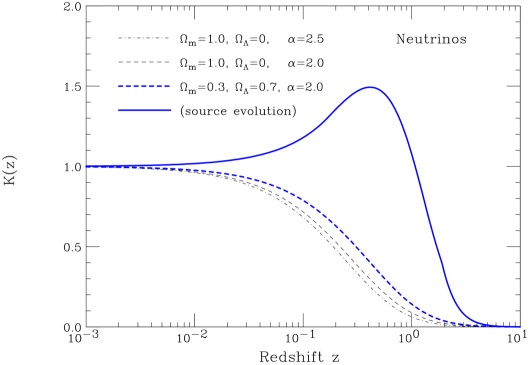
Figure 7: Plot of the redshift response (“Kepler–Olbers”) function $K_{\phi}(z)=K_{\Phi}(z)$ for neutrinos assuming a power law emission of slope $\alpha$. In three of the calculations the neutrino emission is considered constant in time. In a fourth calculation the neutrino emission changes in time with the redshift dependence shown in fig. 6.

Some examples of the redshift response (or Kepler–Olbers) function for neutrinos emitted with a power law spectrum of slope $\alpha$ ($q(E)\propto E^{-\alpha}$) are shown in figure 7. In this particular case (no energy loss except for the redshift effects, and a featureless injection spectrum) the redshift response is independent from energy and one has:

$$K_{\phi}(z)=K_{\Phi}(z)=\frac{(1+z)^{-\alpha}}{{\cal H}(z)}~{}~{}\frac{{\cal L}(z)}{{\cal L}(0)}$$ (62)

As a consequence also the “shape factors” $\zeta_{\phi}=\zeta_{\Phi}$ are equal to each other and independent from energy. This means that an injected power law spectrum of neutrinos is not deformed by propagation effects. As numerical examples, for a matter dominated cosmology ($\Omega_{\rm m}=1$, $\Omega_{\Lambda}=0$) and no source evolution one has:

$$\zeta_{\phi}(\alpha)=\zeta_{\Phi}(\alpha)=\frac{2}{2+\alpha}$$ (63)

Softer spectra (larger slope $\alpha$) have a smaller value of $\zeta_{\phi}$. For the concordance cosmology ($\Omega_{\rm m}=0.3$, $\Omega_{\Lambda}=0.7$) the shape factors are larger by approximately 30%, for example for $\alpha=2$ and no evolution $\zeta_{\phi}=0.5326$. The inclusion of source evolution can on the other hand increase the value of the shape factor by a significant factor. For example using the same redshift dependence of the AGN X–ray luminosity of shown in figure 6 the shape factor for neutrinos increases by a factor $\simeq 4$ (for $\alpha=2$ one finds $\zeta_{\Phi}\simeq 2.2$).

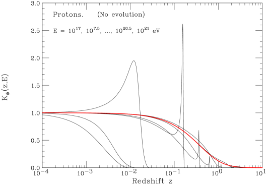
Figure 8: Plot of the redshift response (“Kepler–Olbers”) function $K_{\phi}(z,E)$ for protons assuming a power law emission of slope $\alpha=2.3$. The different curves are calculated (in the absence of source evolution) for different values of the observed proton energy. The thick (red) curve is the curve calculated for neutrinos (considering only redshift energy losses).

The redshift response for protons has a much more complex and interesting structure. Figure 8 shows the redshift response function $K_{\phi}(z,E)$ for values of the proton energy. One can see that for sufficiently low energy $E\lesssim 10^{17}$ eV, the function takes the same form as for neutrinos, since the role of $p\gamma$ interactions becomes negligible. With increasing energy the range of redshift that contribute to the flux becomes progressively smaller. Note also how the energy loss effects enhace the role of a narrow range of redshifts where the high energy tail of the emission rapidly lose energy.

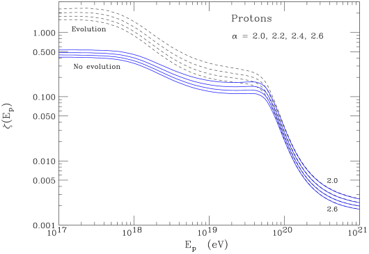
Figure 9: Shape factor $\zeta_{\phi}(E)$ for protons, calculated for a power injection with slope $\alpha=2.0$, 2.2, 2.4 and 2.6. The solid lines are calculated for a constant value of the source power density, while the dashed lines assume for ${\cal L}_{p}(z)$ the redshift dependence shown in fig. 6.

Figure 9 shows the energy dependence of the factor $\zeta_{\phi}(E)$. For energies much smaller that $E\simeq 10^{18}$ eV the factor $\zeta_{\phi}(E)$ reaches an asymptotic value that is in fact equal to the one for neutrino, while at larger energies the effect of $\zeta_{\phi}(E)$ is to distort the power law injection spectrum. The factor $\zeta_{\phi}(E)$ plays therefore the role of a “shape factor” that marks the “imprints” on energy loss on the observable energy spectrum. Berezinsky and his collaborators Berezinsky:2005cq have discussed how this spectral distortion distortion could be the origin of the “ankle” structure observed in the CR flux.

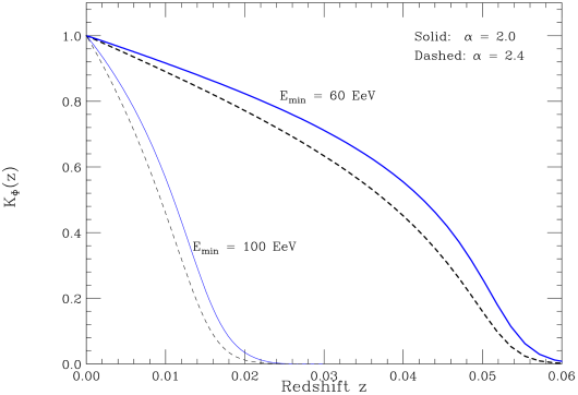
Figure 10: Redshift dependence of the Kepler–Olbers functions $K_{\Phi}(z,E_{\rm min})$ for $E_{\rm min}=6\times 10^{19}$ eV (thick curves) and $E_{\rm min}=10^{20}$ eV (thin curves). The solid (dashed) curves assume a power law injection spectrum with a slope $\alpha=2.0$ ($\alpha=2.4$). Integrating over $z$ one obtain the values $\zeta_{\Phi}=0.037$ (0.034) for $E_{\rm min}=6\times 10^{19}$ eV and $\zeta_{\Phi}=0.0107$ (0.0093) for $E_{\rm min}=10^{20}$ eV.

Figure 10 shows the Kepler–Olbers function $K_{\Phi}(z,E_{\rm min})$ for the integral flux for two values of $E_{\rm min}$ ($E_{\rm min}=6\times 10^{19}$ eV and $10^{20}$ eV); the proton injection spectrum is a power law with slope $\alpha=2.0$ and 2.4. At these very high energies only a small volume of the universe is observable, and the size of this observable volume changes very rapidly with the threshold energy. Integrating over $z$ one obtains (for $\alpha=2.0$) $\zeta_{\Phi}=0.037$ for $E_{\rm min}=6\times 10^{19}$ eV and $\zeta_{\Phi}=0.0107$ for $E_{\rm min}=10^{20}$ eV. For the softer spectra ($\alpha=2.4$) $\zeta_{\Phi}$ shrinks by approximately 10%.

The calculation of the inclusive flux as an integral over redshift:

$$\phi(E)=\frac{R_{0}}{4\,\pi}~{}q_{\rm incl}(E)~{}\int_{0}^{\infty}dz~{}K_{\phi}(z,E)=\frac{R_{0}}{4\,\pi}~{}q_{\rm incl}(E)~{}\zeta_{\phi}(E)$$ (64)

suggests the most useful definition of an energy dependent redshift horizon using the implicit equation:

$$\int_{0}^{z^{\rm hor}_{f}}dz~{}K_{\phi}(z,E)=f~{}\zeta_{\phi}(E)$$ (65)

For example $z^{\rm hor}_{0.9}(E)$ is the redshift that contains the emission of 90% of the protons that are observed with energy $E$. Note that this definition of the horizon depends on the assumed shape of the emission spectrum.

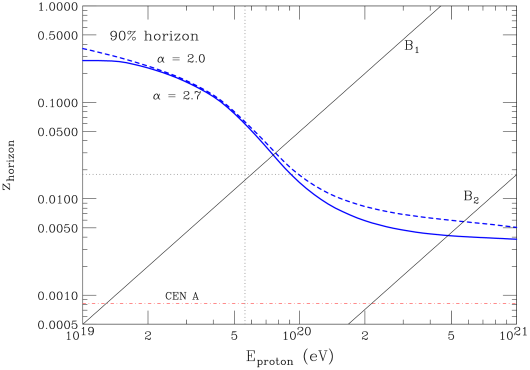
Figure 15: The thick curves show the redshift horizon as a function of the proton energy. The horizon is defined as the value of $z$ within which 90% of the observed flux is emitted. The solid (dashed) line is calculated for a power law emission with slope $\alpha=2.7$ (2.0). The dotted curves indicate the selection criteria used by the Auger collaboration in their correlation analysis Cronin:2007zz . The redshift that corresponds to the Cen A position is also indicated. The curves labeld $B_{1}$ and $B_{2}$ correspond to an expected deviation of 3 degrees with the estimates of the extragalactic magnetic field of equation (22) and (24).

Figure 15 shows the 90% redshift horizon as a function of the proton energy, assuming injection with a power law of slope $\alpha$. In the same figure we show also the energy dependence of the imaging radius (for a 3^∘ resolution) calculated for the two estimates of the parameters $B\sqrt{\lambda_{B}}$ of equations (22) and (24). Proton astronomy is going to be limited to a region $z<z_{\rm hor}(E)$ and $z<z_{\rm magnetic}(E)\simeq R_{\rm imaging}(E)/R_{0}$.

VII The Intensity and Multiplicity distributions

If the universe is filled with a homogeneous distribution of sources, an observer will see an ensemble of objects with a broad distribution of flux intensity, with the faintest (brighest) objects corresponding to the most distant (closest) sources.

In the following we will consider the the integral flux above a fixed threshold energy $E_{\rm min}$. In the following expressions the dependence on this minimium energy will be left implicit. If all sources have the same spectral shape, the distribution $dN_{s}/d\Phi$ that gives the number of sources observable with flux in the interval $[\Phi,\Phi+d\Phi]$ can be written in the form:

$$\frac{dN_{s}}{d\Phi}=\frac{N_{\rm Hubble}}{\Phi_{0}}~{}~{}G_{\Phi}\left(\frac{\Phi}{\Phi_{0}}\right)$$ (66)

where the adimensional constant $N_{\rm Hubble}$:

$$N_{\rm Hubble}=4\,\pi\;R_{0}^{3}~{}\frac{{\cal L}(0)}{L_{0}}$$ (67)

is proportional to the number of sources in one Hubble volume, and the flux $\Phi_{0}$:

$$\Phi_{0}=\frac{Q_{0}}{4\pi\,R_{0}^{2}}=\frac{L_{0}~{}\eta}{4\,\pi\;R_{0}^{2}\;E_{\rm min}}$$ (68)

is the flux from a “typical source” (chosen here as the source with the median luminosity $L_{0}$) placed at the Hubble distance and calculated neglecting all cosmological and energy loss effects. The general expression for $G_{\Phi}(x)$ is:

$$G_{\Phi}(x)=\int_{0}^{\infty}dz~{}\frac{r^{2}(z)}{{\cal H}(z)}~{}~{}\int_{0}^{\infty}dy~{}f_{L}(y,z)~{}\delta\left[x-y~{}F_{\Phi}(z)\right]~{}.$$ (69)

In this expression $r(z)$ and ${\cal H}(z)$ depend on the cosmological parameters, $F_{\Phi}(z)$ is the “dimming function” (defined in equation (30)) and $f_{L}(y,z)$ is the (scaled) luminosity functions (see equation (48)). The function $G_{\Phi}(x)$ encodes the shape of the emission spectrum, the properties of particle propagation and the luminosity function and cosmic evolution of the sources.

As a simple check of this expression one can compute the inclusive particle flux is obtained integrating over all fluxes $\Phi$ the distribution:

$$\Phi_{\rm incl} = \frac{1}{4\,\pi}\int_{0}^{\infty}d\Phi~{}\Phi~{}\frac{dN_{s}}{d\Phi}=N_{\rm Hubble}~{}\Phi_{0}~{}\int_{0}^{\infty}dx~{}x~{}G_{\Phi}(x)$$ (70)

This expression is identical to the result (60) because the integral over $x$ $x\;G_{\Phi}(x)$ is equal to $\zeta_{\Phi}$. In fact, using the definition of $G_{\Phi}(x)$ of equation (69) one finds:

$$\int_{0}^{\infty}dx~{}x~{}G_{\Phi}(x) = \int_{0}^{\infty}dz~{}\frac{r^{2}(z)}{{\cal H}(z)}~{}F_{\Phi}(z)~{}\left(\int_{0}^{\infty}dy~{}y~{}f_{L}(y,z)\right)$$ (71)

$$= \int_{0}^{\infty}dz~{}\frac{r^{2}(z)}{{\cal H}(z)}~{}F_{\Phi}(z)~{}\frac{{\cal L}(z)}{{\cal L}(0)}=\zeta_{\Phi}$$

To be in closer contact with the observations, we will consider an explicit model of detector, described by the effective area $A(\Omega)$ and a finite observation time $t$ and study the number of sources $N_{k}$ detected with exactly $k$ (an integer quantity) events. The multiplicity distribution $N_{k}$ can be obtained starting from the function $dN_{s}/dm$, where $m$ (a real, continuosly varying quantity) is the expected signal from a source. The quantity $dN_{s}/dm$ gives the number of sources with expected signal in the interval $[m,m+dm]$. The probability to detect $k$ events from a source with expected signal $m=\langle k\rangle$ can be obtained using Poissonian statistics. The expected number of events with multiplicity $k$ is therefore:

$$N_{k}=\int_{0}^{\infty}dm~{}\left(e^{-m}~{}\frac{m^{k}}{k!}\right)~{}\frac{dN_{s}}{dm}~{},$$ (72)

the number of multiplets with multiplicity $k\geq 2$ is:

$$N_{\rm multi}\equiv N_{\geq 2}=\int_{0}^{\infty}dm~{}[1-e^{-m}\;(1+m)]\;\frac{dN_{s}}{dm}$$ (73)

and the total number of detected sources is:

$$N_{\rm sources}\equiv N_{\geq 1}=\int_{0}^{\infty}dm~{}[1-e^{-m}]\;\frac{dN_{s}}{dm}$$ (74)

For the calculation of the function $dN_{s}/dm$ we can observe that the expected signal $m$ from a source of luminosity $L$, redshift $z$ and celestial coordinates $\Omega$ is:

$$m(L,z,\Omega)=\Phi(L,z)\;A(\Omega)\,t=~{}\Phi_{0}~{}\frac{L}{L_{0}}~{}F_{\Phi}(z)\;A(\Omega)\,t=\frac{L\;\eta}{4\,\pi\;R_{0}^{2}\;E_{\rm min}}\;F_{\Phi}(z)\;A(\Omega)\,t$$ (75)

The complication here is that in general the detector exposure depends on the celestial coordinates. A simple modeling of the average effective area of the Auger detector and of neutrino telescopes as a function of celestial declination is discussed in appendix A. We will use the notation:

$$A(\Omega)=\langle A\rangle\;a(\Omega)=\frac{A_{\Omega}}{4\,\pi}~{}a(\Omega)$$ (76)

where $\langle A\rangle$ is the detector average effective area, $A_{\Omega}$ is the angle integrated effective area (in units cm² sr) and $a(\Omega)$ is a dimensionless function that satisfies the normalization condition:

$$\int\frac{d\Omega}{4\,\pi}~{}a(\Omega)=1$$ (77)

The distribution $dN_{s}/dm$ can then be written as:

$$\frac{dN_{s}}{dm}=\frac{N_{\rm Hubble}}{m_{0}}~{}~{}G_{m}\left(\frac{m}{m_{0}}\right)$$ (78)

with $N_{\rm Hubble}$ defined in equation (67) and:

$$m_{0}=\Phi_{0}\;\langle A\rangle\;t=\frac{L_{0}~{}\eta}{4\,\pi\;R_{0}^{2}\;E_{\rm min}}~{}\langle A\rangle\;t$$ (79)

The “scaling structure” of equations (66) and (78) can be easily deduced with simple dimensional analysis observing also that the number of sources must be proportional to the quantity ${\cal L}(0)/L_{0}$ that is itself proportional to the source density, and that the signal from any source is linear in the observation time $t$, the detector size (proportional to $\langle A\rangle$), and the source luminosity $L$.

The function $G_{m}(x)$ can be calculated as the convolution:

$$G_{m}(x)=\int\frac{d\Omega}{4\,\pi}~{}\frac{1}{a(\Omega)}~{}G_{\Phi}\left(\frac{x}{a(\Omega)}\right)$$ (80)

Another way to express the same result is:

$$G_{m}(x)=\int\frac{d\Omega}{4\,\pi}~{}\int_{0}^{\infty}dz~{}\frac{r^{2}(z)}{{\cal H}(z)}~{}~{}\int_{0}^{\infty}dy~{}f_{L}(y,z)~{}\delta\left[x-y\;a(\Omega)~{}F_{\Phi}(z)\right]$$ (81)

The function $G_{m}(x)$ satisfies the “sum rule”:

$$\int_{0}^{\infty}dx~{}x~{}G_{m}(x)=\left(\int\frac{d\Omega}{4\,\pi}~{}a(\Omega)\right)~{}\left(\int_{0}^{\infty}dx~{}x~{}G_{\Phi}(x)\right)=\int_{0}^{\infty}dx~{}x~{}G_{\Phi}(x)=\zeta_{\Phi}$$ (82)

As a consistency check one can compute the total number of detected events as:

$$N_{\rm events} = \int_{0}^{\infty}dm~{}m~{}\frac{dN_{s}}{dm}=N_{\rm Hubble}~{}m_{0}~{}\int_{0}^{\infty}dx~{}x~{}G_{m}(x)$$ (83)

$$= \left(\frac{R_{0}}{4\,\pi}~{}\frac{{\cal L}(0)\;\eta}{E_{\rm min}}~{}\zeta_{\Phi}\right)~{}A_{\Omega}\;t=\Phi_{\rm incl}~{}A_{\Omega}\;t$$

The result is simply the inclusive flux (already calculated in equation (60)) times the total detector exposure $A_{\Omega}\;t$, as it must be. Note that the total number of detected events does not depend on the luminosity function of the sources, but only on the (space averaged) emissivity, and also that the result is independent from the geometry or “field of view” of the detector.

The shape of the functions $G_{\Phi}(x)$ or $G_{m}(x)$ in general is complicated, since it encodes the properties of particle propagation, the source luminosity function and, in the case of $G_{m}(x)$, also the detector geometry, however the limit of large $x$ (that is the largest fluxes or signals) the functions have simple asymptotic behaviours:

$$G_{\Phi}(x)\longrightarrow\frac{x^{-5/2}}{2}~{}\langle y^{3/2}\rangle$$ (84)

and

$$G_{m}(x)\longrightarrow\frac{x^{-5/2}}{2}~{}\langle y^{3/2}\rangle~{}\langle a^{3/2}\rangle$$ (85)

where the quantity

$$\langle y^{3/2}\rangle=\int_{0}^{\infty}dy~{}y^{3/2}~{}f_{L}(y,0)$$ (86)

depends on the luminosity function, and

$$\langle a^{3/2}\rangle=\int\frac{d\Omega}{4\,\pi}~{}a^{3/2}(\Omega)$$ (87)

depends on the detector location and geometry. These physically intuitive results can be easily obtained computing the euclidean/static limits of equations (69) and (81) with three steps: (i) use the asymptotic (small $z$ expression) $r^{2}(z)/{\cal H}(z)\to z^{2}$; (ii) approximate the function $F_{\Phi}(z)\to z^{-2}$; and (iii) neglect the redshift dependence of the scaled luminosity function $f_{L}(y,z)\to f_{L}(y)$. The integral over redshift can then be performed using the delta function, and:

$$\int dz~{}z^{2}~{}\delta\left[x-\frac{a}{z^{2}}\right]=\left[z^{2}~{}\left|\frac{2\,a}{z^{3}}\right|^{-1}\right]_{z=\sqrt{a/x}}=\frac{a^{3/2}}{2}~{}x^{-5/2}$$ (88)

The $m^{-5/2}$ ($\Phi^{-5/2}$) behaviour of the distribution of expected signal (flux) remains valid only for sufficiently large signals (fluxes), then the distribution stops growing so quickly for decreasing $m$, and the corrected distribution is integrable down to $m\to 0$.

The number of sources with and expected signal larger than the minimum value $\bar{m}$ can be calculated integrating the distribution $dN_{s}/dm$: in the interval $m\geq\bar{m}$. If $\bar{m}$ is sufficiently large one can use the asymptotic form (85) with the result:

$$N_{s}(\geq\bar{m})=\int_{\bar{m}}^{\infty}dm~{}\frac{dN_{s}}{dm}\simeq~{}\frac{4\,\pi}{3}\frac{{\cal L}(0)}{L_{0}}~{}R_{0}^{3}~{}\left(\frac{m_{0}}{\bar{m}}\right)^{3/2}~{}\left\langle a^{3/2}\right\rangle~{}\left\langle y^{3/2}\right\rangle$$ (89)

This result has a very transparent meaning if one considers the limit of isotropic acceptance and identical source luminosity; then the factors $\langle a^{3/2}\rangle$ and $\langle y^{3/2}\rangle$ become unity, the quantity ${\cal L}/L_{0}$ is simply the source density, and the result takes the form

$$N_{s}(\geq m)\to n_{s}~{}\frac{4\,\pi}{3}~{}R_{m}^{3}$$ (90)

where

$$R_{m}=R_{0}~{}\left(\frac{m_{0}}{\bar{m}}\right)^{1/2}=\left(\frac{L_{0}\;\eta~{}\langle A\rangle\,t}{4\,\pi\;E_{\rm min}}~{}\frac{1}{m}\right)^{1/2}$$ (91)

is the radius (in static, euclidean space) of the sphere at wich the signal has value $m$. Note that the radius $R_{m}$ is independent from the Hubble distance $R_{0}$, as it must be, since it is calculated neglecting cosmological effects.

Similarly, the expected number of sources that yield a “multiplet” of multiplicity $k\geq 2$ can be calculated using the asymptotic form of $G_{m}$ with the result:

$$N_{\rm multiplets}=\int_{0}^{\infty}dm~{}[1-e^{-m}\,(1+m)]~{}\frac{dN_{s}}{dm}\simeq\sqrt{\pi}~{}N_{s}(m\geq 1)$$ (92)

where we have used the result:

$$\int_{0}^{\infty}dm~{}[1-e^{-m}\,(1+m)]~{}\frac{m^{-5/2}}{2}=\frac{\sqrt{\pi}}{3}~{}$$ (93)

The expected number of multiplets can be well approximated as the number of sources with an expected signal larger than unity, multiplied by a factor $\sqrt{\pi}$. The limit of validity of the approximation (92) will be discussed later.

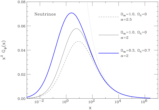
Figure 11: Plot of the function $G_{\phi}(x)=G_{\Phi}(x)$ for neutrinos observations. The neutrino emission has a power law form with slope $\alpha$, and all neutrino sources have identical luminosity. The different curves are calculated for different cosmological parameters, and for two different values of the slope $\alpha$. The dotted curve show the function $x^{-5/2}/2$.

Some examples of the function $G_{\Phi}(x)$ calculated for neutrino sources assuming a power law emission, and all identical sources are shown in fig. 11. The function $G_{\Phi}(x)$ is calculated for two different set of values of the cosmological parameters (a matter dominated universe and the concordance cosmology) and two different value of the slope $\alpha$. One can see that for $x$ large the function takes the “universal shape” $G_{\Phi}(x)\to x^{-5/2}/2$, while for sufficiently small $x$ the curve deviates from the “euclidean form”. The small $x$ (or faint source part) of the function is not universal, but depend on the cosmological parameters and the shape of the emission spectrum.

Figure 12 shows some examples of the $G_{\Phi}(x)$ function calculated for protons, integrating the observed flux above two different threshold energies $E_{\rm min}=6\times 10^{19}$ eV and $E_{\rm min}=10^{20}$ eV. The calculation is performed for an emission spectrum $E^{-2.4}$ with two assumptions about the sources, either all identical sources, or the broad luminosity distribution of equation (45). Again, at large $x$ the function takes its universal form $x^{-5/2}/2$ for a fixed source luminosity or $x^{-5/2}\langle y^{3/2}\rangle/2$ for a luminosity distribution. However for protons this euclidean behaviour stops at a larger $x$, because of the effect of energy loss. In fact for the higher energy threshold, the euclidean behaviour is valid in a smaller range of $x$.

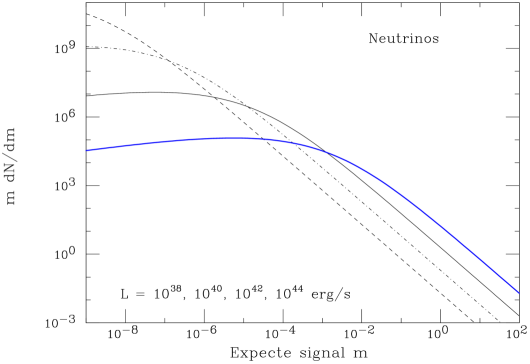
Figure 13: Number of sources with an expected signal $m$ (plotted in the form $m\;dN/dm$ versus $m$). The distributions are calculated for the sam, power density ${\cal L}_{\nu}$, assuming that all sources have the same luminosity $L$ and emit with a a power law spectrum of slope $\alpha=2$, The different curves differ only because of the value of $L$.

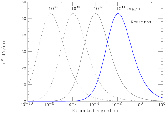
Figure 14: As in figure 13, but plotted in the form $m^{2}\;dN/dm$ versus $m$. The area under each curve is proportional to the total number of detected neutrino events.

For a qualitative understanding of the role of the function $G_{m,\Phi}(x)$ one can look at figures 13 and 14 that show the distribution of expected signal $m=\Phi\,A\,t$ for an isotropic neutrino detector. Neutrinos are emitted by an ensemble of identical sources of luminosity $L_{0}$ emitting with a power law spectrum of slope $\alpha=2$; the cosmological parameters are $\Omega_{m}=1$ and $\Omega_{\Lambda}=0$. The injection power density ${\cal L}$ is taken to the same value, but different calculations assume different values for the luminosity $L_{0}$ of the individual sources. Changing $L_{0}$ leaves the total signal unchanged, but generates very different distributions $dN/dm$. Figure 14 shows the distribution $dN/dm$ is the form $m^{2}\,dN/dm$ versus $m$ with a logarithmic scale for $m$. In this way the area under the cuve is proportional to inclusive signal and the shape of the curve is identical to the shape of the curve $x^{3}\;G_{\Phi,m}(x)$. It is simple to see that the power density of the sources change the absolute normalization of the curve, the luminosity $L_{0}$ “shifts” the distribution to higher or smaller signals, with the overall shape determined by the scaling function $G_{\Phi}(x)$ that is calculable from the particle propagation properties, the cosmological parameters, and the shape of the luminosity function.

VIII Interpretation of the data on UHECR clustering

It is possible to use the instruments developed in the previous sections to analyse the results obtained by UHECR detectors. As an example we will discuss the results of the Auger detector for the first integrated exposure $A_{\Omega}\;t=9000$ (Km² yr sr) Cronin:2007zz ; Abraham:2007si . In this exposure the detector has observed 27 events with energy above $E_{\rm th}\simeq 6\times 10^{19}$ eV. From this event rate it is possible to estimate the power density ${\cal L}_{p}(E_{\rm th})$ of the emission in the energy interval [$E_{\rm th},\;10\,E_{\rm th}]$ making the assumptions that the particles are protons, and using equation (83) that can rewritten as:

$$N_{\rm events}=17.2~{}\left(\frac{{\cal L}_{p}(E_{\rm th})}{10^{36}~{}{\rm erg}/{\rm s}\;{\rm Mpc}^{3}}\right)~{}\left(\frac{A_{\Omega}\;t}{9000~{}{\rm Km}^{2}~{}{\rm yr}~{}{\rm sr}}\right)~{}\left(\frac{\zeta_{\Phi}(E_{\rm th})}{0.037}\right)~{}\left(\frac{\eta}{0.434}\right)$$ (94)

From the observed event rate one can estimate the power density is:

$${\cal L}_{p}(E_{\rm th})\simeq 1.6\times 10^{36}~{}\left(\frac{E_{\rm th}}{60~{}{\rm EeV}}\right)~{}\left(\frac{0.037}{\zeta_{\Phi}(E_{\rm th})}\right)~{}\left(\frac{0.434}{\eta}\right)~{}\frac{{\rm erg}}{{\rm s}~{}{\rm Mpc}^{3}}$$ (95)

The error on the determination of the power density is dominated by systematic effects associated with uncertainties in the determination of the energy scale of the measurement. An error in the energy scale affects obviously the value of $E_{\rm th}$, in addition, the value of the shape factor $\zeta_{\Phi}(E_{\rm th})$ is a very steep function of energy. For $E\sim E_{\rm th}$ this energy dependence can be approximated with $\zeta_{\Phi}(E)\propto E^{-2.3}$. Therefore one can make estimate the uncertainty on the power density as:

$$\frac{\Delta{\cal L}_{p}(E_{\rm th})}{{\cal L}_{p}(E_{\rm th})}\simeq 0.20~{}({\rm stat})+3.3~{}\left(\frac{\Delta E}{E}\right)_{\rm scale}$$ (96)

The shape of the CR energy spectrum is also important. It determines the quantity $\eta$ that connects the integral emission and the power density ($Q_{\rm incl}(E_{\rm th})={\cal L}(E_{\rm th})\;\eta/E_{\rm th}$), and also the precise value of the shape factor $\zeta_{\Phi}(E_{\rm th})$. If the spectrum is a power law with a slope that varies in the interval $\alpha\in[2,2.6]$ then $\eta$ (see equation (41)) varies in the interval $\eta\in[(\ln 10)^{-1}=0.434,~{}0.500]$, with a steeper spectrum requiring less power for the same flux. For the same range of slope, the shape factor $\zeta_{\Phi}(E_{\rm th})$ (for $E_{\rm th}=60$ EeV) varies in the interval $\zeta_{\Phi}\in[0.037,0.032]$, in this case a steeper spectrum has a smaller horizon and therefore requires more power to generate the same flux. The effects of changing the slope $\alpha$ go in opposite directions for $\eta$ and $\zeta_{\Phi}$ and therefore in first approximation cancel each other in the estimate of the power density.

The determination of the shape of the extragalactic flux of CR requires the disentangling of the galactic component. A crucial problem is the determination of the transition energy where the two components (galactic and extragalactic) are equal. If the transition energy corresponds to the “ankle” at $E\simeq 10^{19}$ eV, the slope of the spectrum is only poorly determined experimentally. Theoretical prejudice has traditionally favored a flat slope $\alpha\simeq 2$. If the extragalactic component dominates down to much lower energy as advocated first by Berezinsky and his collaborators Berezinsky:2005cq , the slope $\alpha$ is better determined and is significantly larger than 2. If the evolution of the sources is negligible, one estimates $\alpha\simeq 2.6$, if the source evolution has a behaviour similar to the Stellar Formation Rate (or the AGN luminosity function) one obtains $\alpha\simeq 2.4$.

If uncertainties in the spectral shape are not very significant in the estimate of the power density in the energy decade above 60 EeV, they have a very dramatic effect if one attempts to estimate a total CR power density integrated over all energies. Extrapolating the power low behaviour to the interval $\{E_{\rm min},E_{\rm max}\}$ one can easily compute:

$${\cal L}_{p}[E_{\rm min},E_{\rm max}]={\cal L}_{p}[E_{\rm th},10\,E_{\rm th}]~{}\frac{\eta}{(\alpha-2)}~{}\left[\left(\frac{E_{\rm min}}{E_{\rm th}}\right)^{-\alpha+2}-\left(\frac{E_{\rm max}}{E_{\rm th}}\right)^{-\alpha+2}\right]$$ (97)

In the limit of $\alpha=2$ this becomes:

$${\cal L}_{p}[E_{\rm min},E_{\rm max}]={\cal L}_{p}[E_{\rm th},10\,E_{\rm th}]~{}\frac{\ln(E_{\rm max}/E_{\rm min})}{\ln 10}$$ (98)

with a weak, logarithmic dependence on the energy limits. If $\alpha$ is large the low energy extension of the spectrum is problematic because the energy requirement grows rapidy with decreasing $E_{\rm min}$, in good approximation $\propto(E_{\rm min}/E_{\rm th})^{-\alpha+2}$. As an illustration the extension as an unbroken power law of the extragalactic CR spectrum down to $E_{\rm min}\simeq 10^{12}$ eV requires a power approximately 9 (2100) times larger than the estimate of equation (95) if one assumes a slope $\alpha=2$ ($\alpha=2.4$).

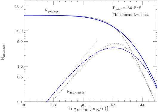
Figure 16: Expected total number of detected sources (solid lines) and number of sources with multiplicity $k\geq 2$ (dashed lines) plotted as a function of the median luminosity of the sources. The calculation assumes a threshold energy $E_{\rm min}\simeq 6\times 10^{19}$ eV and a total exposure of 9000 (Km² yr sr) for the Auger detector. The source power density is set to ${\cal L}_{p}\simeq 1.6\times 10^{36}$ erg/(s Mpc³) to reproduce the observed event rate. The thin (thick) curves assumed a fixed luminosity (the luminosity function of equation (45). The dotted line is $\propto\sqrt{L_{0}}$.

The clustering of the events detected above the threshold energy $E_{\rm th}=6\times 10^{19}$ eV can give us information about how the power density (95) is subdivided in individual sources if we assume that the propagation of protons of these energies for distances of the order of the corresponding horizon is approximately linear. The general method to compute the expected number of clusters with multiplicity $N_{k}$ has been discussed before, and involves the calculation of the distribution of expected signal $dN_{s}/dm$, and the folding with a Poissonian probability. The results of a numerical calculation of $N_{\rm multi}$ (the number of clusters with multiplity $k\geq 2$) and of detected sources as a function of the median luminosity $L_{0}$ is shown in figure 16. The calculation is performed for the value of the source power density that reproduces the inclusive rate, and using two models for the luminosity function: a fixed luminosity, and the broad luminosity distribution given in equation (45) and shown in figure 5.

The behaviour of the curves $N_{\rm sources}(L_{0})$ is simple to understand qualitatively. For small $L_{0}$ the cosmic ray signal is given by the contribution of many faint sources, each contributing a small fraction of an event and one has $N_{\rm sources}\simeq N_{\rm events}$, with a negligible probability of observing multiplets. Increasing $L_{0}$ the number of detected sources (for a fixed power density) decreases monotonically as the number density of sources decreases, while the volume contained inside the horizon remains fixed.

The behaviour of $N_{\rm multi}(L_{0})$ as a function of $L_{0}$ shows a maximum for $L_{0}=L_{0}^{*}\sim 10^{42}$ erg/s. For a median luminosity $L_{0}\ll L_{0}^{*}$ the number of multiplets grows $\propto L_{0}^{1/2}$ according to equation:

$$N_{\rm multi} = \sqrt{\pi}~{}\left(\frac{4\,\pi}{3}\right)~{}{\cal L}_{p}(E_{\rm th})~{}\sqrt{L_{0}}~{}~{}\left(\frac{\eta\;A_{\Omega}\,t}{16\,\pi^{2}\;E_{\rm min}}\right)^{3/2}~{}\langle a^{3/2}\rangle~{}\langle y^{3/2}\rangle$$ (99)

$$\simeq 0.74~{}\left(\frac{{\cal L}(0)}{10^{36}\;{\rm erg}/{\rm s}\;{\rm Mpc}^{3}}\right)~{}\sqrt{\frac{L_{0}}{10^{40}~{}{\rm erg}/{\rm s}}}~{}\left(\frac{A_{\Omega}\;t}{9000~{}{\rm Km}^{2}\;{\rm yr}\;{\rm sr}}\right)^{3/2}\langle y^{3/2}\rangle$$

The behaviour $N_{\rm multi}\propto\sqrt{L_{0}}$ has a very simple explanation. The radius of the sphere within which a source of luminosity $L_{0}$ is sufficiently bright to generate a multiplet grows approximately $\propto\sqrt{L_{0}}$, accordingly the volume that contains multiplets grows $\propto L_{0}^{3/2}$; on the other hand, for a fixed luminosity density the number density of the sources is $n_{s}\propto L_{0}^{-1}$, with the combined result $N_{\rm multi}\propto L_{0}^{3/2}~{}L_{0}^{-1}\propto L_{0}^{1/2}$. This behaviour stops when the radius of detection of a source becomes comparable with the “horizon radius” of order $(R_{0}\,\zeta_{\Phi})$. Additional increase in $L_{0}$ decreases the number of the multiplets, since the detection volume remains approximately constant while the source number density decreases. The coefficient of proportionality between $N_{\rm multi}$ and $\sqrt{L_{0}}$ depends linearly on the factors $\langle a^{3/2}\rangle$ and $\langle y^{3/2}\rangle$. The first, defined in equation (76), depends on the detector geometry and event selection criteria. For the Auger detector location and the cut on zenith angle $\theta<60^{\circ}$ one has $\langle a^{3/2}\rangle\simeq 1.26$. The factor $\langle y^{3/2}\rangle=1$ is unity if all sources have the same luminosity; for the broad luminosity distribution (45) $\langle y^{3/2}\rangle\simeq 1.64$. It is intuitive that a broad luminosity distribution (with large $\langle y^{3/2}\rangle$) yields a larger number of multiplets than a narrow one thanks to the contribution of high luminosity sources in the tail of the distribution.

In the regime of validity of equation (99) It is possible to obtain $L_{0}$ with a simple, closed form expression as a function of $N_{\rm events}$ and $N_{\rm multi}$ solving the system composed of equations (83) and (99):

$$L_{0} \simeq 144\,\pi~{}\left(\frac{N_{\rm multi}}{N_{\rm events}}\right)^{2}~{}\frac{E_{\rm th}~{}[R_{0}\;\zeta_{\Phi}(E_{\rm th})]^{2}}{\eta~{}(A_{\Omega}\;t)}~{}\frac{1}{\langle a^{3/2}\rangle^{2}}~{}\frac{1}{\langle y^{3/2}\rangle^{2}}$$ (100)

Substituting the number of events observed in Auger one finds:

$$L_{0}\simeq 7.5\times 10^{39}~{}\frac{(N_{\rm multi})^{2}}{\langle y^{3/2}\rangle^{2}}~{}\left(\frac{E_{\rm th}}{60~{}{\rm EeV}}\right)~{}~{}\left(\frac{\zeta_{\Phi}(E_{\rm th})}{0.037}\right)^{2}~{}~{}\frac{\rm erg}{\rm s}$$ (101)

Note that in the regime of validity of this equation the number of multiplets grows with time as: $N_{\rm multi}\propto t^{3/2}$, while the number of events is $N_{\rm events}\propto t$, therefore the combination [$(N_{\rm multi}/N_{\rm events})^{2}\;t^{-1}$] is a constant. The behaviour $L_{0}\propto(N_{\rm multi}/N_{\rm events})^{2}$ loses is validity for $L_{0}\gtrsim 10^{41}$ erg/s, when sources not too distant from the energy loss horizon begin to be visible.

The question of how the 27 highest energy events detected by Auger can be subdivided into the contribution of different sources has not a simple answer, and is intimately related to the problem of the the deviations of the particles during their propagation and the size of the extragalactic magnetic fields.

The “nominal interpretation” of the Auger events, suggests that particles with $E\gtrsim 60$ EeV are deviated by approximately 3 degrees, and therefore that the clustering of events should be searched for using a correlation cone of approximately this size. If one tentatively accepts this conclusion, defining a cluster as a set of events with angular separation less than a $3^{\circ}$, one finds 2 doublets and correspondingly 23 singlets. Increasing the size of the correlation cone to 5^∘ one finds one triplet and three doublets, while the 18 remaining events are singlets. These numbers should be corrected for the effect of random coincidences that in turn depends on the assumptions about the larger scale angular distribution of the flux. Taken at face value these results, together with the the calculations shown in figure 16 suggest an allowed range for the luminosity $L_{0}$:

$$10^{39}~{}\frac{\rm erg}{\rm s}\lesssim L_{0}\lesssim 10^{41.5}~{}\frac{\rm erg}{\rm s}$$ (102)

The lower limit follows from the fact that (at a modest confidence level) some clustering is observed. The upper limit follows from the fact that most of the events are actually in singlets, and that the total number of objects that contribute to the signal is larger than $\simeq 20$.

In fact the Auger data suggest that at least one source of UHECR has been established with a very high degree of confidence. The position of the very close Active Galactic Nucleus Cen A coincides with the most prominent of all tentative clustering structures (the triplet found for a 5^∘ aperture cone). Considering that Cen A, on the basis of its properties and closeness to the Earth, has been proposed as one of the most likely sources of UHECR this is a striking result. The detection of Cen A is an remarkable result of historic importance. It is the first imaging of an astrophysical object with charged particles and, 4 centuries after the invention of the optical telescope and 20 years after the detection of SN1987A with neutrinos, marks the birth of a new astronomy.

The clarification of the size and structure of the excess of events from the Cen A direction is very important to evaluate the perspectives of the field of CR astronomy. In fact it is possible that Cen A accounts for a number of events larger than 2 or 3. For example a 10^∘ ($20^{\circ}$) cone around the direction of Cen A contains 4 (9) events, suggesting that the excess from this direction is larger and more extended. It should be stressed that Cen A is remarkably close to us with a distance of only 3.5 pc. Since the deviations of a particle during propagation in intergalactic space scales as $\sqrt{d}$ (with $d$ the sorce distance) a signal with an angular size of several degrees from Cen A suggest that astronomy from sources at larger distances will be very difficult and require higher energies. The result is also in possible conflict with the correlation cone of 3.2 degrees found between the direction of the highest energy cosmic ray and the position of AGN with $z\leq 0.017$ found in Cronin:2007zz since the distance of these AGN is typically 20 times larger, and the expected deviation of particles produced in sources is expected to be 4 times larger.

There are several solution to this problem: the apparent large angular size of the event excess in the direction of Cen A could be due to the contributions of other sources in the same portion of the sky; the large angular deviations could be the effect of strong magnetic fields in the vicinity of the source and not in intergalactic space (but of course this should then be expected for a significant fraction of all the other sources); the angular spread of the signal could be associated with the size of the emission region from Cen A that has jets extending several degrees away from its nucleus. It could however also mean that the intergalactic magnetic fields are stronger than expected, and that cosmic ray extragalactic astronomy is only possible only for very close sources or very high energy.

In any case, the power emitted in cosmic ray from CenA is straightforward to compute. In fact the source is so close to us that the cosmological and energy loss corrections are small for $E\sim 6\times 10^{19}$ eV. The luminosity in the energy decade above $E_{\rm min}$ can be estimated as:

$$L_{\rm CenA}\simeq 1.5\times 10^{39}~{}\left(\frac{N_{\rm CenA}}{2}\right)~{}\left(\frac{d}{3.5~{}{\rm pc}}\right)^{2}~{}\frac{\rm erg}{\rm s}$$ (103)

(where $N_{\rm CenA}$ is the number of events arriving from Cen A). This result is in reasonable agreement (at least in order of magnitude) with the estimates (101) and (102), especially allowing for a broad luminosity distribution.

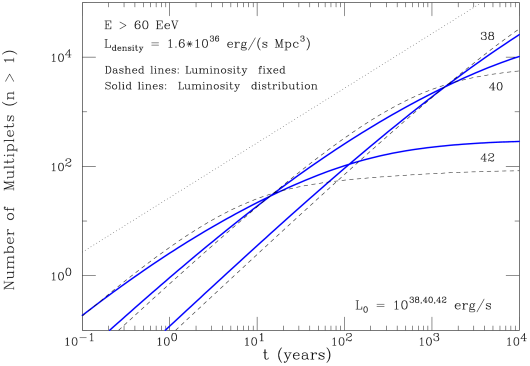
Figure 17: Expected number of proton sources detectable in Auger with multiplicity $n\geq 2$ (for $E_{\rm min}=6\times 10^{19}$ eV) plotted as a function of detector live time. The power density of the sources is ${\cal L}_{p}=1.6\times 10^{36}$ erg/(s Mpc³). to reproduce the observed inclusive event rate (the dotted line gives the total number of events as a function of time). The different curves are calculated assuming that all sources have the same spectral shape (a power law of slope $\alpha=2.0$) and 3 possible values of the median luminosity: ($L_{0}=10^{38}$, $10^{40}$ and $10^{42}$ erg/s). The dashed line are calculated with a fixed luminosity, while the solid lines are the result using the luminosity function of equation (45) and shown in fig. 5.

It is interesting to make a prediction on how the number of detected clusters will scale with additional exposure. An illustration of this problem is in fig. 17 that shows how the number of clusters with multiplicity $n\geq 2$ grows with exposure for the Auger detector. If the median luminosity of the sources is small the number of clusters grows $\propto(A\,t)^{3/2}$, faster than the linear growth of the inclusive rate. Eventually this growth must slow down and finally stop when the exposure is sufficient to observe as clusters of events sources close to the energy loss horizon. The asymptotic number of detectable sources is clearly sensitive to the form of the luminosity function, and to the density of weak sources with luminosity much smaller than the median luminosity $L_{0}$.

IX Extragalactic neutrinos

The existence of the extragalactic cosmic rays is the best reason to predict also a measurable flux of extragalactic neutrinos. In fact, the CR sources must unavoidably also generate neutrinos, because a fraction of the relativistic hadrons they produce will interact with matter or radiation fields inside or near the source, producing weakly decaying particles (pions and kaons) that generate neutrinos. The power density and luminosity function of the neutrino extragalactic sources are therefore related to the analogous quantities for cosmic ray emission. The relation between the CR and the $\nu$ emissions is very uncertain and depends on the structure of the sources. The motivation for the simultaneous measurement of both cosmic rays and neutrinos is precisely the understanding of the nature and structure of their common sources.

In the following we want to discuss the observations of neutrinos using the detection of $\nu$–induced muons in “Km³” type neutrino telescopes like IceCube at the South Pole and Km3Net in the Mediterranean sea. We will use a simplified model for the effective area of a neutrino detector that is discussed in appendix B. It can be useful to think about the signal of neutrino induced muons as a measurement of the integral neutrino flux above the threshold $E_{\nu}^{\rm min}\simeq 1$ TeV using an effective area that is the geometric area of the detector times an energy averaged neutrino to muon conversion efficiency of order $\langle\varepsilon_{\nu\to\mu}\rangle\sim 3\times 10^{-6}$. The exact value of $\langle\varepsilon_{\nu\to\mu}\rangle$ depends on the shape of the neutrino spectrum, the energy threshold for muon detection and the average zenith angle of the source considered. Taking into account the small conversion efficiency the effective area of a Km³ neutrino detector is of order of only few square meters, many orders of magnitude smaller that the effective area of a telescope like Auger (with a surface of approximately 3000 Km²). It is however interesting to note that, in some sense, the sensitivities of detectors like Auger and IceCube are comparable. This can be illustrated with the following example, if we have one source that emits protons and neutrinos with spectra that are approximately equal in both shape and absolute normalization, and the spectra can be reasonably well approximated as power law of slope $\alpha\simeq 2$, the the source (if in the field of view of the detectors) will leave event rates in ultra high energy showers, and in neutrino induced muons are of the same order of magnitude. This can be easily understood qualitatively observing that energy threshold shower detection is of order $\sim 10^{20}$ eV, while the neutrino telescopes is sensitive to neutrinos with $E_{\nu}\gtrsim 10^{12}$ eV. The integral fluxes above these energy thresholds are (for a spectrum of slope $\alpha\simeq 2$) in a ratio $10^{-8}$, but also the effective areas differ by approximately the same factor, resulting in approximately the same event rates.

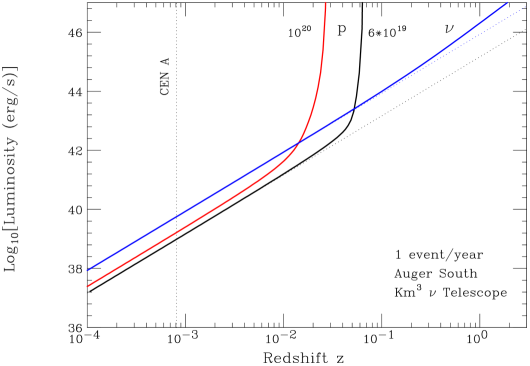
Figure 18: The lines describe the curves in the {$z$, $L$} (luminosity, distance) plane that correspond to a rate of one event/year from a source. The luminosity must be understood as luminosity per energy decade. The different curves are for the detection of proton showers with threshold energy $E_{\rm min}=60$ and 100 EeV in Auger (assuming a source declination $\delta\simeq-30\circ$), and for the number of neutrino induced muons in IceCube (for a source with $\delta>0$). The dotted lines are $\propto z^{2}$.

This discussion is made more quantitative in figure 18 that show the curves in the plane $\{z,L\}$ (distance, luminosity) that corresponds to one event/year in Auger (for a source places at $\delta\simeq-30^{\circ}$) and in a Km³ telescope of the IceCube type. The luminosity must be understood as the luminosity per energy decade, and the source spectrum is a power law with slope $\alpha=2$. For very close sources, the lines that correspond to a constant event rate have the simple form $L(z)z^{2}\simeq{\rm const}$. For these close sources, the neutrino event rate is a factor approximately 5 (3) times smaller than the shower rate with a threshold $E=6\times 10^{19}$ eV ($E=10^{20}$ eV). On the other hand the proton source become effectively invisible when they are behind an energy loss horizon that is a rapidly varying function of energy, while the entire universe is visible with neutrinos.

It is interesting to perform also for extragalactic neutrinos the same study done for protons, and discuss what fraction of the inclusive signal can be resolved as the contribution of individual sources.

With respect to the study of UHECR there are a several obvious differences. The first one is that neutrinos travel in straight lines and therefore the problem of the impact of extragalactic magnetic field is entirely absent. The angular size of a cluster of $\nu$–induced muons is controled by the muon–neutrino angle, that is calculable (the angular dimension of the signal has a weak but non entirely negligible dependence on the shaope of the neutrino spectrum).

A second difference is the presence of the atmospheric neutrino background that constitute an important complication. The total number of neutrino events from astrophysical sources can only be obtained with a non trivial analysis that requires the estimate and subtraction of the background.

An additional problem is that much (but not all) of the information about the shape of the neutrino energy spectrum is lost. The detected muon energy can only be measured with poor resolution, and this energy is only poorly correlated with the parent neutrino energy.

Finally, neutrinos can travel without interacting across a Hubble distance, and it is therefore expected that the fraction of the inclusive signal that can be resolved and associated to individual sources, is going to be much smaller than for UHECR that can reach us only from a much smaller volume determined by the energy loss length.

At present there is only an upper limits on the possible flux of extragalactic neutrinos. The most stringent one has been obtained by the Amanda detector at the South Pole Achterberg:2007qp , and is expressed in reference to an isotropic neutrino spectrum of form $\phi_{\nu}=K_{\nu}~{}E^{-2}$. The 90% C.L. upper limit on the constant $K_{\nu_{\mu}}$ (relevant for the combination $\nu_{\mu}+\overline{\nu}_{\mu}$) is

$$K_{\nu_{\mu}}\equiv E^{2}~{}\phi_{\nu_{\mu}}\leq 7.4\times 10^{-8}~{}{\rm GeV}/({\rm cm}^{2}\;{\rm s}\;{\rm sr})$$ (104)

The quantity $K_{\nu_{\mu}}$ can be expressed in terms of the power density of the neutrino sources at the present epoch using:

$$3~{}K_{\nu_{\mu}}=\frac{R_{0}}{4\,\pi}\;\frac{{\cal L}_{\nu}^{0}}{\ln 10}~{}\zeta_{\Phi}$$ (105)

where the factor of 3 takes into account the expected contribution of all other neutrino flavors (see Lipari:2007su for a critical discussion). The upper limit on the power density of the extragalactic neutrino sources is:

$${\cal L}_{\nu}^{0}\lesssim 1.04\times 10^{37}~{}~{}\left(\frac{2.2}{\zeta_{\Phi}}\right)~{}\frac{\rm erg}{{\rm Mpc}^{3}\;{\rm s}}$$ (106)

(The estimate $\zeta_{\Phi}\simeq 2.2$ includes an important redshift dependence of the source power density). It can be useful to translate this upper limit on the extragalactic neutrino flux as a maximum number of events generated from extragalactic neutrinos. The total number of extragalactic neutrino events can be calculated using equations (83), and depends on the power density of the neutrino events:

$$N_{\rm events} \simeq 1270~{}\left(\frac{{\cal L}_{\nu}^{0}}{10^{37}~{}{\rm erg}/({\rm Mpc}^{3}{\rm s})}\right)~{}\left(\frac{\zeta_{\Phi}}{2.2}\right)~{}\left(\frac{\varepsilon_{\nu\to\mu}}{3\times 10^{-6}}\right)~{}\left(\frac{\eta}{0.434}\right)~{}\left(\frac{A_{0}~{}t}{{\rm km}^{2}~{}{\rm yr}}\right)~{}~{}~{}~{}$$ (107)

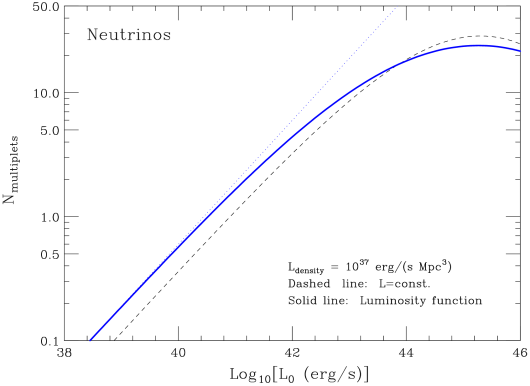
Figure 19: Expected number of neutrino event clusters with $k\geq 2$ plotted as a function of the median luminosity $L_{0}$ of the neutrino sources. The calculation is performed with a neutrino power density ${\cal L}_{\nu}^{0}=10^{37}$ erg/(s Mpc³), and assuming no cosmological evolution of the sources. The solid lines assume the luminosity function of equation (45), the dashed lines a fixed value $L=L_{0}$.

A calculation of the number of sources and of the number of multiplets as a function of the median luminosity $L_{0}$ is shown in fig. 19. The calculation is performed for a power density of the neutrino sources ${\cal L}_{\nu}^{0}=10^{37}$ erg/(s Mpc³) just below the existing constraints. For $L_{0}$ not too large the expected number of multiplets is proportional to $\sqrt{L_{0}}$ according to the approximationo of equation (99) that can be recast in numerical form as:

$$N_{\rm multi} \simeq 3.7~{}\left(\frac{{\cal L}_{\nu}^{0}}{10^{37}~{}{\rm erg}/({\rm Mpc}^{3}{\rm s})}\right)~{}\sqrt{\frac{L_{0}}{10^{42}~{}{\rm erg}/{\rm s}}}~{}\left(\frac{A_{0}~{}t}{{\rm km}^{2}~{}{\rm yr}}\right)^{3/2}~{}\langle y^{3/2}\rangle$$ (108)

In equation (108) the quantity $\langle a^{3/2}\rangle$ has been estimated as $\sqrt{2}$. This value is valid for IceCube that observes only half of the sky. For a neutrino telescope placed in the mediterranean sea at a latitude of approximately 36^∘ one can estimate $\langle a^{3/2}\rangle\simeq 1.11$, that is 20% lower. For a neutrino detector placed at the equator one should have $\langle a^{3/2}\rangle\simeq 1$. The dependence of the expected number of resolve sources on the detector latitude is an elementary geometric effect associated with the reduced field of view of a detector close to the poles. A detector that observes only a fraction $1/n$ of the celestial sphere (with constant effective area in this portion of the sky) has $\langle a^{3/2}\rangle=\sqrt{n}$. The “horizon” of such a detector is $\sqrt{n}$ time deeper that the horizon of a detector that observes the entire sky with the same angle integrated exposure, and the number of observed sources scales as the volume contained inside the horizon, that is $n^{-1}\times n^{3/2}=\sqrt{n}$ larger that for an isotropic detector. Deeper observations of a smaller fraction of the sky yield more resolved sources.

The number of multiplets is also proportional to the total number of events. This relation can be written as:

$$N_{\rm multi} = N_{\rm events}~{}\frac{1}{6\,\sqrt{2}\;R_{0}}\left[\frac{A_{0}\;t\;\langle\varepsilon_{\nu\to\mu}\rangle\;L_{0}\;\eta}{E_{\rm min}}\right]^{1/2}~{}\frac{\langle a^{3/2}\rangle~{}\langle y^{3/2}\rangle}{\zeta_{\Phi}}$$ (109)

$$= 2.9\times 10^{-3}~{}~{}\sqrt{\frac{L_{0}}{10^{42}~{}{\rm erg}/{\rm s}}}~{}\sqrt{\frac{A_{0}~{}t}{{\rm Km}^{2}{\rm yr}}}~{}\left(\frac{2.2}{\zeta_{\Phi}}\right)~{}\langle y^{3/2}\rangle~{}N_{\rm events}$$

This can also be rewritten as a function of the quantity $K_{\nu_{\mu}}=E^{2}~{}\phi_{\nu_{\mu}}(E)$:

$$N_{\rm multi} = 0.47\;\left(\frac{K_{\nu_{\mu}}}{10^{-8}\;{\rm GeV}/{\rm cm}^{2}{\rm s}{\rm sr}}\right)~{}\sqrt{\frac{L_{0}}{10^{42}\;{\rm erg}/{\rm s}}}\;\left(\frac{A_{0}~{}t}{{\rm km}^{2}~{}{\rm yr}}\right)^{3/2}\;\left(\frac{2.2}{\zeta_{\Phi}}\right)\;\langle y^{3/2}\rangle$$ (110)

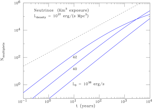
Figure 20: Expected number of extragalactic neutrino sources detectable in IceCube with a multiplicity of up–going muons $n\geq 2$ plotted as a function of detector live time. The neutrino sources are all identical and emit with power law spectra with slope $\alpha=2$ and a luminosity per energy decade $L_{0}$. The power density of the ensemble of all neutrino sources is ${\cal L}=10^{37}$ erg/(s Mpc³). The different curves are calculated for different values $L_{0}=10^{38}$, $10^{40}$ and $10^{42}$ erg/s. The dashed line give the inclusive number of detected up–going muons that are produced by extragalactic neutrinos. For a detector places in the Mediterranean sea at a latitude of $36^{\circ}$ the number of sources should be reduced by a factor 0.787.

For completeness, figure 20 shows a prediction of the evolution of the number of clusters of neutrino induced muons produced by extragalactic neutrino sources with increasing exposure. The number of multiplets is expected to grow approximately $\propto(A\,t)^{3/2}$ even for exposures of hundreds of square kilometer year. This is a consequence of the fact that this functional form continues until the detector sensitivity is sufficient to see as muon multiplets sources located at approximately a Hubble distance, and this does require very large exposures, unless the luminosity of the source is extraordinarily large.

X Outlook

The key problems about the nature and properties of the extragalactic cosmic rays sources remain open, even if some of the answers seems to be tantalizingly close. One of the most urgent problems is the determination of the region of source distance and particle energy where astronomy with charged cosmic rays is possible. The results of Auger on the correlation of the arrival direction of the highest energy CR with the positions of close AGN suggest that astronomy with CR is possible with a threshold of $\sim 6\times 10^{19}$ eV, and a volume of radius $R\simeq 75$ Mpc. These are very encouraging results, but they need to be confirmed with more statistics. If a significant part of the anisotropy effect observed by Auger is due to the contribution of a single source at only 3.5 pc the observation of more distant sources could be significanly more problematic.

Assuming that the linear propagation of the highest energy cosmic rays is a reasonable approximation and that most of the particles are protons, the clustering (and lack of clustering) of the highest energy events determinee to within a factor of 300 or so the typical luminosity of a extragalactic CR sources (in the energy decade above $E\simeq 6\times 10^{19}$ eV) as $L_{0}\in[10^{39},10^{41.5}]$ erg/s. This is not inconsistent with the estimated luminosity of Cen A that is of order few times $10^{39}$ erg/s. In the same energy region the power density of the ensemble of the CR sources if of order of $1--2\times 10^{36}$ erg/(s Mpc³).

The neutrino observations, that at present limit the power density of the neutrino sources to a maximum value of order ${\cal L}_{\nu}\lesssim 10^{37}$ erg/(s Mpc³) offer already a quite significant constraint, since the neutrino limit refer to the power density per energy decade in at much lower energy, and therefore suggest that the spectrum of the CR emission cannot extend to low energy with a too steep spectrum. The inclusive extragalactic neutrino flux is mostly generated by distant, very faint sources, and therefore only a small fraction (probably less than $10^{-3}$) can be resolved in the contribution of individual sources by detectors of the IceCube type. If an extragalactic neutrino component is not too far from the existing upper limits, the sensitivity of the Km³ neutrino telescopes could be insufficient to detect more than a handful of extragalactic sources.

Acknowledgments I would like to acknowledge discussions with Steve Barwick, Maurizio Lusignoli, Andrea Silvestri and Todor Stanev.

Appendix A Detector Acceptance for EAS Arrays

The geometry of an Extensive Air Shower Array (EAS) is sufficiently simple that it is possible to have a reasonably accurate description of its acceptance with simple analytic expressions. In this type of detection method, cosmic ray showers are analysed if their zenith angle is smaller than a maximum value $\theta_{\rm max}$, and if the shower axis falls inside a predetermined region of area $A_{0}$. The effective area for the detection of showers coming from a direction with zenith angle $\theta$ is therefore $A(\theta)\simeq A_{0}\;\cos\theta$. The angle integrated area is:

$$A_{\Omega}=A_{0}~{}2\pi\;\int_{\cos\theta_{\rm max}}^{1}d\cos\theta~{}\cos\theta=A_{0}~{}\pi\,\left[1-(\cos\theta_{\rm max})^{2}\right]$$ (111)

The Auger detector has used the cut $\theta_{\max}=60^{\circ}$, and therefore its integrated exposure is approximately:

$$A_{\Omega}\simeq A_{0}~{}\left(\frac{3\,\pi}{4}\right)$$ (112)

The interesting problem is to compute the detector acceptance as a function of the celestial direction. This can be done taking into account the trajectories in the detector system of points with different coordinates on the celestial sphere. All points with the same celestial declination $\delta$ make the same trajectory in the sky with zenith angle:

$$\cos\theta(h,\delta,\varphi_{\rm lat})=\cos\delta\;\cos\varphi_{\rm lat}\;\cos h+\sin\delta\;\sin\varphi_{\rm lat}$$ (113)

($h$ is the hour angle). Averaging over one sidereal day and taking into account only of the time when a celestial direction is sufficiently high above the horizon, one can compute the “average” effective area for points with declination $\delta$ as:

$$\langle A(\delta)\rangle=A_{0}~{}\langle\cos\theta(\delta,\varphi_{\rm lat})\rangle=A_{0}~{}\int_{0}^{2\pi}\frac{dh}{2\pi}~{}\cos\theta(h,\delta,\varphi_{\rm lat})~{}\Theta\left[\cos\theta-\cos\theta_{\rm max}\right]$$ (114)

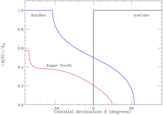
Figure 21: Plot of the detector effective area $A(\Omega)$ as a function of the celestial declination $\delta$. In the case of the Auger–South detector, the effective area is divide by the surface area of the array, the detector latitude is $\varphi_{\rm lat}=-24.8^{\circ}$ and the projected area is averaged for the time when a source has zenith angle $\theta<60^{\circ}$. For the neutrino telescopes, the detector projected area in the direction $\theta$ is approximated as constant, and $\nu$ detection is considered possible for all zenith angles $\theta>90^{\circ}$.

The averaging over a sidereal day is a good approximation for long periods of data taking. The function $\langle\cos\theta(\delta,\varphi_{\rm lat}\rangle$ for the latitude of the Auger detector ($\varphi_{\rm lat}\simeq 24.8^{\circ}$) is shown in fig. 21. Integrating the acceptance over all the celestial sphere one must obtain the same result as integrating over the detector angular coordinates, and therefore one obtains (for any detector latitude) the relation:

$$\int_{-\pi/2}^{\pi/2}d\delta\cos\delta~{}\langle\cos\theta(\delta,\varphi_{\rm lat})\rangle=\frac{1}{2}\,\left[1-(\cos\theta_{\rm max})^{2}\right]$$ (115)

Appendix B Neutrino detection

The most promising technique for the detection of point–like astrophysical neutrinos sources is the observations of $\nu$–induced muons. These muons are produced in the charged current interactions of $\nu_{\mu}$ and $\overline{\nu}_{\mu}$ in the matter below the detector, and are approximately collinear with the parent neutrino direction, and therefore excellent tools for the imaging of neutrino sources.

The $\nu$–induced muon signal is detectable only eliminating the large background of atmospheric muons due to the decay of charged pions and kaons produced in the hadronic showers of cosmic rays interacting in the Earth’s atmosphere. This can be achieved limiting the neutrino observations to up–going trajectories. With this limitation, a neutrino telescope placed at the South Pole can only observe the northern celestial hemisphere.

The signal of astrophysical neutrinos remains partially hidden by the background of atmospheric neutrinos that has the same origin of the muon background (the weak decays of hadronic produced by cosmic ray showers). The astrophysical neutrino signal can however be disentangled from this background because of its different (harder) energy spectrum. Point sources can be identified as clusters of events with approximately the same direction.

In this work, following Lipari:2006uw , we will consider a simplified description of neutrino detection that is sufficient for our discussion. We will assume that the neutrino energy can be reasonably well described in the relevant energy range ($10^{12}\lesssim E_{\nu}\lesssim 10^{16}$ eV) as a simple power law of slope $\alpha$. The flux of muons generated by neutrinos with spectrum $\phi_{\nu}(E_{\nu})$ can be calculated as:

$$\Phi_{\mu}(E^{\rm min}_{\mu})=\int dE_{\nu}~{}\frac{\phi(E_{\nu})}{6}\left[P_{\rm surv}^{\nu_{\mu}}(E_{\nu},\theta)~{}Y_{\nu_{\mu}\to\mu^{-}}(E_{\nu},E^{\rm min}_{\mu})\right.$$

$$\left.~{}~{}~{}~{}~{}~{}~{}~{}~{}~{}~{}~{}~{}~{}~{}~{}~{}~{}~{}~{}~{}~{}~{}~{}~{}~{}~{}~{}~{}~{}~{}~{}~{}~{}~{}~{}+P_{\rm surv}^{\overline{\nu}_{\mu}}(E_{\nu},\theta)~{}Y_{\overline{\nu}_{\mu}\to\mu^{+}}(E_{\nu},E^{\rm min}_{\mu})\right]$$ (116)

In this expression $\phi_{\nu}(E_{\nu})$ is the neutrino flux summed over all $\nu$ types, and the factor 1/6 follows from the assumption that flavor oscillations mix the neutrinos, so that one has approximately equal amounts for each type ($\nu_{e}$, $\overline{\nu}_{e}$ $\nu_{\mu}$, $\overline{\nu}_{\mu}$ $\nu_{\tau}$ and $\overline{\nu}_{\tau}$). For a critical discussion of this result see for example Lipari:2007su . The function $P_{\rm surv}^{\nu_{\mu}}(E_{\nu})$ ($P_{\rm surv}^{\overline{\nu}_{\mu}}(E_{\nu})$) is the probability that a $\nu_{\mu}$ ($\overline{\nu}_{\mu}$) that arrives at the detector with zenith angle $\theta$, survives the crossing the Earth without interacting, and $Y_{\nu_{\mu}\to\mu^{-}}(E_{\nu},E_{\mu,{\rm min}})$ ($Y_{\overline{\nu}_{\mu}\to\mu^{+}}(E_{\nu},E_{\mu,{\rm min}})$) is the muon yield, that is the number of muons with $E\geq E_{\mu,{\rm min}}$ generated by a $\nu_{\mu}$ ($\overline{\nu}_{\mu}$) of energy $E_{\nu}$.

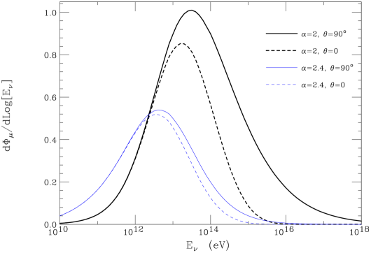
Figure 22: Neutrino energy response for the up–going muon signal. The area under the curves is proportional to the signal of $\nu$ induced muons (with threshold $E_{\mu}=1$ GeV) assuming a power law neutrino flux with slope $\alpha$. The thick (thin) curves are calculated for a slope $\alpha=2$ ($\alpha=2.4$); the solid (dashed) curves are calculated for a nadir angle $\theta=90^{\circ}$ ($\theta=0^{\circ}$) and negligible (maximum) $\nu$ absorption in the Earth. The relative normalization of the curves is correct if the spectra have the same integrated flux above 1 TeV. The $\nu$ induced signal is roughly proportional to the integrated neutrino flux in the approximate energy range $[10^{12},10^{16}]$ eV in case of a hard spectrum, or $[10^{11},10^{15}]$ eV for a soft spectrum.

The integrand of equation (116) is shown in fig. 22, for two examples of the slope $\alpha$ and on the two extreme cases (minimum and maximum) of the effects of absorption in the Earth. Inspection of fig. 22 shows that for a neutrino spectrum of slope not much larger than $\alpha\simeq 2$ the muon signal is generated by neutrinos in the energy range $[10^{12},10^{16}]$ eV. It is therefore useful, at least for a qualitative understanding to consider the flux the neutrino induced muons as proportional to the integral flux of neutrino above a (conventional but roughly appropriate) energy threshold of $E_{\nu}^{\rm min}=10^{12}$ eV, introducing an energy averaged neutrino to muon conversion efficiency $\langle\varepsilon_{\nu\to\mu}\rangle$ that can be calculated performing the ratio between the muon and the neutrino fluxes:

$$\langle\varepsilon_{\nu\to\mu}\rangle=\frac{\Phi_{\mu\uparrow}(E^{\rm min}_{\mu})}{\Phi_{\nu}(E_{\nu}\geq 1~{}{\rm TeV})}$$ (117)

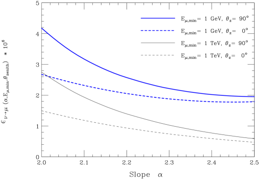
Figure 23: Neutrino to muon conversion efficiency. The different curves correspond to different choices for the muon detection threshold and different celestial declination of a source for a neutrino detector at the South Pole.

The conversion efficiency $\langle\varepsilon_{\nu\to\mu}\rangle$ depends on (i) the muon energy threshold, (ii) the slope of the neutrino spectrum (being higher for flatter spectra), and because of the effects of $\nu$ absorption in the Earth, (iii) on the neutrino zenith angle. This is illustrated in fig. 23) that shows some examples of $\langle\varepsilon_{\nu\to\mu}\rangle$. In the following, we will neglect the zenith angle dependence of $\langle\varepsilon_{\nu\to\mu}\rangle$, considering that this is a reasonable approximation given the size of the astrophysical uncertainties.

For a detector located at the South Pole, the northern celestial hemisphere remains constantly below the horizon and can observed continuosly, while the southern hemisphere in unobservable. The effective area will be simply modeled as:

$$A(\Omega)\simeq\cases{A_{0}~{}\langle\varepsilon_{\nu\to\mu}\rangle&for $\delta>0$\cr 0&for $\delta\leq 0$}$$ (118)

with $A_{0}\simeq 1$ Km². The angle integrated effective area is $A_{\Omega}=2\,\pi\;A_{0}~{}\langle\varepsilon_{\nu\to\mu}\rangle$. For first order numerical estimates in the following we will use $\langle\varepsilon_{\nu\to\mu}\rangle=3\times 10^{-6}$, that is the correct value for a low muon energy threshold and a slope $\alpha\simeq 2.1$. For a flatter spectra with $\alpha\simeq 2.5$, the conversion is smaller: $\langle\varepsilon_{\nu\to\mu}\rangle\simeq 2\times 10^{-6}$.

Figure 5: Shape of the luminosity function that fits the $X$–ray observations of AGN in the [10,20] KeV band (from ueda ).

Figure 6: Redshift evolution of the X–ray luminosity density of AGN in the [10,20] KeV band according to the fit of ueda .

Figure 12: Plot of the function $G_{\Phi}(x)$ (in the form $x^{2}\;G_{\Phi}(x)$ versus $x$) for the proton integral flux. The calculation is performed for a power law energy spectrum with $\alpha=2.4$ and two energy threshold $E_{\rm min}=6\times 10^{19}$ eV and $E_{\rm min}=10^{20}$ eV. The dashed lines are calculated assuming that all sources have the same luminosity, while the solid line assume the luminosity function of equation (45) shown also in fig. 5. The dotted curves show the functions $x^{-5/2}/2$ and $x^{-5/2}\,\langle y^{3/2}\rangle/2$

References

- (1) N. Hayashida et al., Phys. Rev. Lett. 77, 1000 (1996).
- (2) M. Takeda et al., Astrophys. J. 522, 225 (1999) [arXiv:astro-ph/9902239].
- (3) Y. Uchihori, M. Nagano, M. Takeda, M. Teshima, J. Lloyd-Evans and A. A. Watson, Astropart. Phys. 13, 151 (2000) [arXiv:astro-ph/9908193].
- (4) S. L. Dubovsky, P. G. Tinyakov and I. I. Tkachev, Phys. Rev. Lett. 85, 1154 (2000) [arXiv:astro-ph/0001317].
- (5) P. Sommers and S. Westerhoff, arXiv:0802.1267 [astro-ph].
- (6) T. K. Gaisser, F. Halzen and T. Stanev, Phys. Rept. 258, 173 (1995) [Erratum-ibid. 271, 355 (1996)] [arXiv:hep-ph/9410384].
- (7) J. G. Learned and K. Mannheim, Ann. Rev. Nucl. Part. Sci. 50, 679 (2000).
-
(8)
K. Greisen,
Phys. Rev. Lett. 16, 748 (1966).
G. T. Zatsepin & V. A. Kuzmin, JETP Lett. 4, 78 (1966). - (9) J. Abraham et al. [Pierre Auger Collaboration], Science 318, 938 (2007) [arXiv:0711.2256 [astro-ph]].
- (10) J. Abraham et al. [Pierre Auger Collaboration], Astropart. Phys. 29, 188 (2008) [arXiv:0712.2843 [astro-ph]].
- (11) D. S. Gorbunov, P. G. Tinyakov, I. I. Tkachev and S. V. Troitsky, arXiv:0804.1088 [astro-ph].
- (12) A. A. Ivanov et al. [Yakutsk Collaboration] Pisma Zh. Eksp. Teor. Fiz. 87, 215 (2008) [JETP Lett. 87, 185 (2008)] [arXiv:0803.0612 [astro-ph]].
- (13) T. Wibig and A. W. Wolfendale, arXiv:0712.3403 [astro-ph].
- (14) T. Stanev, arXiv:0805.1746 [astro-ph].
- (15) R. U. Abbasi et al., [HiRes Collaboration] arXiv:0804.0382 [astro-ph].
- (16) Y. Ueda et al., Prog.Th.Phys.Supp 155, 209 (2004).
- (17) A. Achterberg et al. [IceCube Collaboration], Phys. Rev. D 76, 042008 (2007) [Erratum-ibid. D 77, 089904 (2008)] [arXiv:0705.1315 [astro-ph]].
- (18) V. Berezinsky, A. Z. Gazizov & S. I. Grigorieva, Phys. Lett. B 612, 147 (2005) [arXiv:astro-ph/0502550].
- (19) P. Lipari, M. Lusignoli and D. Meloni, Phys. Rev. D 75, 123005 (2007) [arXiv:0704.0718 [astro-ph]].
- (20) P. Lipari, Nucl. Instrum. Meth. A 567, 405 (2006) [arXiv:astro-ph/0605535].
- (21) A. Achterberg et al. [IceCube Collaboration], Phys. Rev. D 75, 102001 (2007) [arXiv:astro-ph/0611063].