Geometric quantization of integrable systems with hyperbolic singularities

Abstract

We construct the geometric quantization of a compact surface using a singular real polarization coming from an integrable system. Such a polarization always has singularities, which we assume to be of nondegenerate type. In particular, we compute the effect of hyperbolic singularities, which make an infinite-dimensional contribution to the quantization, thus showing that this quantization depends strongly on polarization.

1 Introduction

In the theory of geometric quantization, the “quantization” of a symplectic manifold $M$ is constructed from sections of a complex line bundle over $M$. The ingredients for geometric quantization are as follows: a symplectic manifold $(M,\omega)$, a complex line bundle $\mathbb{L}$ over $M$, and a connection $\nabla$ on $\mathbb{L}$ whose curvature is $\omega$. We also require a polarization, which is an integrable complex Lagrangian distribution (see [22] for more information). A real polarization is given by a foliation of $M$ into Lagrangian submanifolds. If $\mathcal{J}$ is the sheaf of sections of $\mathbb{L}$ that are covariant constant (with respect to $\nabla$) in the directions tangent to the leaves of the foliation, then the quantization of $M$ is

$$\mathcal{Q}(M)=\bigoplus_{k\geq 0}H^{k}(M;\mathcal{J}),$$

where $H^{*}(M;\mathcal{J})$ is the cohomology of $M$ with coefficients in $\mathcal{J}$.

The main result about quantization using real polarizations is a theorem of Śniatycki [18] from 1975: If the leaf space $B^{n}$ is a manifold and the map $\pi\colon M^{2n}\to B^{n}$ a fibration with compact fibres, then all of these cohomology groups are zero except in degree $n$. Furthermore, $H^{n}$ can be expressed in terms of Bohr-Sommerfeld leaves. A Bohr-Sommerfeld leaf is one on which is defined a global section which is flat along the leaf (see Definition 7). The set of Bohr-Sommerfeld leaves is discrete, and Śniatycki’s result says that the dimension of $H^{n}$ is equal to the number of Bohr-Sommerfeld leaves. (It actually applies to non-compact manifolds as well, in which case the non-zero cohomology is in degree equal to the rank of a fibre of $\pi$. However, in this paper we only consider the compact case.)

The hypothesis that $B^{n}$ be a manifold is quite restrictive, however. For example, in a completely integrable system, by the Arnol’d-Liouville theorem the fibres of the moment map are generically Lagrangian tori, but there may be fibres which have smaller dimension or are not manifolds. This is like a real polarization except for the singularities, and so we view it as a singular real polarization and extend the quantization machinery to this case.

A local classification of the types of nondegenerate singularities appearing in integrable systems has been established by Eliasson and the second author in [5, 7, 15]. It has as starting point the algebraic classification due to Williamson [21] of Cartan subalgebras of the Lie algebra of the symplectic group, and is given in terms of a local model for the components of the moment map near the singularity. Singularities can be written as a product of three basic types, which are called elliptic, hyperbolic, and focus-focus.

In [9], the first author computed the quantization of systems with only elliptic singularities. The result obtained was similar to Śniatycki’s: all cohomology groups are zero except in degree $n$, and $H^{n}$ has dimension equal to the number of Bohr-Sommerfeld leaves. However, the singular Bohr-Sommerfeld leaves do not make a contribution to the cohomology and are not included in this count.

A natural question, then, is what are these cohomology groups for a system with the other types of singularities? This paper addresses the case of hyperbolic singularities in two dimensions. We plan to return to the focus-focus case, and the general case of singularities of mixed types, in a future paper. Note that this paper completes the case of this quantization (with respect to singular real polarizations) for compact manifolds of two dimensions, since focus-focus components can only appear in dimensions four or higher.

The main result of this paper (Theorem 21) is:

Theorem.

Let $(M,\omega,F)$ be a two-dimensional, compact, completely integrable system, whose moment map has only nondegenerate singularities. Suppose $M$ has a prequantum line bundle $\mathbb{L}$, and let $\mathcal{J}$ be the sheaf of sections of $\mathbb{L}$ flat along the leaves. The cohomology $H^{1}(M,\mathcal{J})$ has two contributions of the form $\mathbb{C}^{\mathbb{N}}$ for each hyperbolic singularity, each one corresponding to a space of Taylor series in one complex variable. It also has one $\mathbb{C}$ term for each non-singular Bohr-Sommerfeld leaf. That is,

$$H^{1}(M;\mathcal{J})\cong\bigoplus_{p\in\mathcal{H}}\bigl{(}\mathbb{C}^{\mathbb{N}}\oplus\mathbb{C}^{\mathbb{N}}\bigr{)}\oplus\bigoplus_{b\in BS}\mathbb{C}_{b}.$$ (1)

The cohomology in other degrees is zero. Thus, the quantization of $M$ is given by (1).

We follow the methods of [9], dividing the manifold up into open sets and computing the cohomology of each set individually, and then piecing them together using a Mayer-Vietoris argument. The case of neighbourhoods of regular leaves is covered by the theorems in [18] and [9], so we concentrate on a neighbourhood of a singular leaf, where we compute the cohomology groups using a Čech approach.

One of the issues in geometric quantization is “independence of polarization,” the question of whether different polarizations give equivalent quantizations. When we allow singularities in the polarization, we find that the quantization depends strongly on the polarization, in the sense that we can easily introduce new hyperbolic singularities by using surgery of integrable systems (see §7). We also give explicit examples coming from mechanics of two different systems on a sphere with different quantizations: rotation about the vertical axis, and the Euler equations on the sphere. The first one has no hyperbolic singularities, while the second one has two, giving four infinite-dimensional contributions to the quantization.

The organization of this paper is as follows: We review definitions and terminology in section 2, and prove some properties of the sheaf of flat sections in section 3. The cohomology computation for the simplest hyperbolic system is carried out in sections 4 and 5, and extended to more complicated leaf structures in 6. In section 7 we describe the surgery of integrable systems and give two examples from mechanics with different polarizations having different quantizations. Finally, section 8 contains a technical proof having to do with Čech cohomology.

1.1 Acknowledgements

The acknowledgements part in this paper deserves its own subsection. During the process of working on this project, the authors have been substantially helped by many people along the way. First, a big thanks must go to Victor Guillemin who has helped us a lot with this problem, and has enthusiastically followed up on its progress. We are also extremely grateful to Yael Karshon for the many helpful conversations and suggestions during our visit to Toronto during the early stages of this project. Many thanks also to both Victor and Yael for the invitations to Boston and Toronto which made an important contribution to our work.

We are very grateful to Mathematisches Forschungsinstitut Oberwolfach for the opportunity to work on this project in the beautiful settings of the Institute. Oberwolfach has provided a perfect working atmosphere in the fantastic Black Forest, which gave a beautiful backdrop to our sometimes messy calculations.

Thanks to Jerrold Marsden and Tudor Ratiu who kindly provided us with the lovely picture of the Euler equations (Figure 12) in section 7.2.

Last but not least, we want to thank Roger and Tess from 9 Baldwin Street in Toronto for their hospitality during the early stages of this project.

2 Definitions

2.1 Integrable systems

Let $(M^{2n},\omega)$ be a symplectic manifold of dimension $2n$. The Poisson bracket is defined on $M$ by $\{f_{i},f_{j}\}=\omega(X_{f_{i}},X_{f_{j}})$ where $X_{f_{j}}$ is the Hamiltonian vector field of $f_{j}$. A completely integrable system is given by a set of $n$ functions $f_{1},\dots,f_{n}$ which Poisson commute and which are generically functionally independent.

Since $0=\{f_{i},f_{j}\}=\omega(X_{f_{i}},X_{f_{j}})$ and $[X_{f_{i}},X_{f_{j}}]=X_{\{f_{i},f_{j}\}}=0$, the distribution generated by the Hamiltonian vector fields of the functions $f_{i}$ is involutive and the regular integral manifolds are Lagrangian submanifolds of $(M^{2n},\omega)$.

The collection of functions $F=(f_{1},\dots,f_{n})$ is often called the moment map in the literature of integrable systems. Observe that when the manifold is compact, the moment map $F$ has singularities, which correspond to singularities of the distribution by Hamiltonian vector fields. A whole theory has been developed (and is still being developed) for the singularities of this mapping and the symplectic invariants attached to them. In the case that the singularities are non-degenerate (in the sense of [7]), there is a local symplectic Morse theory for these systems (see [5] and [15]).

If $(M,\omega)$ is two-dimensional, a completely integrable system is just a function $F\colon M\to\mathbb{R}$. In this case, a non-degenerate singular point $p$ is a point where $d_{p}F=0$ and the Hessian $d_{p}^{2}F$ is non-degenerate. There are only two types of non-degenerate singularities for integrable systems in dimension 2: hyperbolic (when the Hessian is indefinite) or elliptic (when the Hessian is positive or negative definite).

The following theorem is due to Colin de Verdière and Vey [4], and is a special case in two dimensions of more general results by Eliasson and the second author ([5, 7, 15]). It gives a symplectic local model for a neighbourhood of the singularity.

Theorem 1.

Let $F\colon(M^{2},\omega)\longrightarrow\mathbb{R}$ be a function and let $p$ be a non-degenerate singular point of $F$. Let $Q$ be the quadratic form corresponding to the Hessian of $F$ at $p$.

Then there exists a local diffeomorphism from a neighbourhood $Z$ of $p$ to a neighbourhood of $0$ in $\mathbb{R}^{2}$ taking $\omega$ to the symplectic form $dx\wedge dy$ and $F$ to a function $\phi(Q)$. If the hessian $Q$ is positive definite the germ of the function $\phi$ characterizes the pair $(F,\omega)$. If $Q$ is not definite then the jet at the point $p$ of the function $\phi$ characterizes the pair $(F,\omega)$.

Remark 2.

As a consequence of this theorem, after putting $Q$ in a canonical form, we can assume from now on that the foliation in a neighbourhood of a singular point $p$ corresponding to $0\in\mathbb{R}^{2}$ is given by the vector field

• $Y=-y\frac{\partial}{\partial x}+x\frac{\partial}{\partial y}$ when $Q=x^{2}+y^{2}$ ($p$ is elliptic) or

• $Y=x\frac{\partial}{\partial x}-y\frac{\partial}{\partial y}$ when $Q=xy$ ($p$ is hyperbolic)

and the symplectic form is $\omega=dx\wedge dy$. We call these $x$-$y$ coordinates “Eliasson coordinates.”

In the case that $p$ is hyperbolic, we usually take $Z$ to be a “hyperbolic cross” (see Figure 1), what Toulet in [6] calls an “étoile canonique.”

Figure 1: A “hyperbolic cross”

2.2 Geometric quantization

Let $(M,\omega)$ be a symplectic manifold. A prequantization line bundle is a complex line bundle $\mathbb{L}$ over $M$, equipped with a connection $\nabla$ whose curvature is $\omega$. A real polarization is a foliation of $M$ into Lagrangian submanifolds. (For a more complete description of geometric quantization, see [22] or [19].)

Suppose $(M,\omega,F)$ is a compact completely integrable system. We wish to compute the quantization of $M$ using the singular real polarization given by the singular foliation by levels of $F$, which (as noted in the Introduction) are generically Lagrangian tori.

Definition 3.

A section $\sigma$ of $\mathbb{L}$ is flat along the leaves or leafwise flat if it is covariant constant along the fibres of $F$, with respect to the prequantization connection $\nabla$. This means that $\nabla_{X}\sigma=0$ for all $X$ tangent to fibres of $F$. Denote by $\mathcal{J}$ the sheaf of smooth sections which are flat along the leaves.

Definition 4.

With $(M,\omega,F)$, $\mathbb{L}$, and $\mathcal{J}$ as above, the quantization of $M$ is

$$\mathcal{Q}(M)=\bigoplus_{k\geq 0}H^{k}(M;\mathcal{J}).$$

Remark 5.

In the theory of geometric quantization as originally developed independently by Kostant and Souriau, the quantum space was the section of “polarized” sections of $\mathbb{L}$ (which correspond to our leafwise flat sections). However, with a real polarization with compact leaves, there are no global polarized sections (see the proof of Theorem 20). One solution to this problem, suggested by Kostant in [11], is to look at higher cohomology, which is what we do.

A note on terminology: We have two rivals for the term “flat” in this paper. We will distinguish them by specifying leafwise flat as above, versus analytically flat as follows:

Definition 6.

A function is Taylor flat or analytically flat (at some specified point, which is often understood) if it vanishes to infinite order at that point, that is, if all of its Taylor coefficients are zero.

Our results will be expressed in terms of Bohr-Sommerfeld leaves.

Definition 7.

A leaf $\ell$ of the (singular) foliation is a Bohr-Sommerfeld leaf if there is a leafwise flat section $\sigma$ defined over all of $\ell$.

Note that, while leafwise flat sections always exist locally (because the curvature of $\nabla$ is $\omega$, which is zero when restricted to a leaf), the condition of existing globally is quite strong. The set of Bohr-Sommerfeld leaves is discrete (in the leaf space). Note also that a leaf is Bohr-Sommerfeld iff its holonomy is trivial around all loops contained in the leaf.

3 The leafwise flat sections

We first prove several properties of elements of the sheaf $\mathcal{J}$, which will be instrumental in what follows. In particular, sections in $\mathcal{J}$ are analytically flat in particular ways: see Propositions 9 and 11. For all of this section (and indeed, the rest of this paper), $Z$ denotes the neighbourhood of the hyperbolic singular point given in Theorem 1.

Lemma 8.

We may choose a trivializing section of the prequantization line bundle $\mathbb{L}$ over $Z$ so that the potential one-form of the prequantum connection is $\Theta_{0}=\tfrac{1}{2}(x\,dy-y\,dx)$ in Eliasson coordinates.

Remark.

Remember that the potential one-form $\Theta$ of a connection, relative to some trivialization, is defined as follows: If $s$ is the trivializing section, and $\sigma=\psi s$ is a section, then

$$\nabla_{X}\psi s=\bigl{(}X(\psi)-i\psi\Theta(X)\bigr{)}s.$$ (2)

Proof of Lemma 8.

Since $Z$ is contractible, $\mathbb{L}$ is trivializable over $Z$. Let $s$ be a trivializing section, and let $\Theta$ be the potential one-form on $Z$ defined by (2). Since the curvature of the connection is $\omega$, $d\Theta=\omega=d\Theta_{0}$, and so $\Theta-\Theta_{0}$ is closed on $Z$ and, therefore, exact. Write $dg=\Theta-\Theta_{0}$, and define a new trivialization $s_{0}$ of $\mathbb{L}$ over $Z$ by $s_{0}=e^{ig}s$. Writing a section $\sigma$ as $\psi_{0}s_{0}$, it is easy to check that

$$\nabla_{X}\psi_{0}s_{0}=\bigl{(}X(\psi_{0})-i\psi_{0}\Theta_{0}(X)\bigr{)}s_{0}$$

and so $\Theta_{0}$ is the potential one-form of $\nabla$ with respect to $s_{0}$. ∎

Proposition 9.

If $\sigma\colon Z\to\mathbb{L}$ is a smooth leafwise flat section defined over $Z$, then $\sigma$ is Taylor flat at the singular point. That is,

$$\frac{\partial^{j+k}\sigma}{\partial^{j}x\,\partial^{k}y}\biggr{\rvert}_{(0,0)}=0\quad\text{for all }j,k$$

Proof.

According Theorem 1, the foliation by level sets is generated by

$$Y=x\frac{\partial}{\partial x}-y\frac{\partial}{\partial y}.$$

Take a trivializing section $s$ of $\mathbb{L}$ as in Lemma 8, so that the prequantum connection can be written

$$\nabla_{X}(\sigma)=X(\sigma)-i\Theta_{0}(X)\sigma$$

(where here $\sigma$ represents a complex-valued function). Thus any leafwise flat section $\sigma$ must satisfy the equation

$$Y(\sigma)=-ixy\sigma.$$

Writing $\sigma=\sigma_{1}+i\sigma_{2}$ with $\sigma_{1}$ and $\sigma_{2}$ both real, we obtain the following two equations:

$$\begin{split}Y(\sigma_{1})&=xy\sigma_{2}\\ Y(\sigma_{2})&=-xy\sigma_{1}\end{split}$$ (3)

Let $\sum_{ij}a_{ij}x^{i}y^{j}$ be the Taylor expansion of $\sigma_{1}$ and $\sum_{ij}b_{ij}x^{i}y^{j}$ the Taylor expansion of $\sigma_{2}$. We want to see that $a_{ij}=0$ and $b_{ij}=0$ $\forall i,j$. In order to do that we plug the Taylor expansions into the system (3), and obtain, for all $i,j$, the following system of equations for the $a_{ij}$ and $b_{ij}$:

$$\begin{split}(i-j)a_{ij}&=b_{i-1,j-1}\\ (i-j)b_{ij}&=a_{i-1,j-1}\end{split}$$ (4)

We distinguish two cases:

1. $i=j$. In this case, we obtain immediately $b_{i-1,i-1}=0$ and $a_{i-1,i-1}=0$, for all $i$.

2. $i\neq j$. In this case, combining and solving equations (4) yields:

   $$b_{ij}=\frac{-b_{(i-2)(j-2)}}{(i-j)^{2}}.$$

   Now iterating this process $k$ times we obtain:

   $$b_{ij}=\frac{(-1)^{k}b_{(i-2k)(j-2k)}}{(i-j)^{2k}}.$$

   Now let $k$ be such that $i<2k$, then $b_{(i-2k)(j-2k)}=0$ since the coefficients of the Taylor-Laurent expansion of a smooth function vanish for negative subindexes.

From this, we obtain $b_{ij}=0$ for all $i,j$ and therefore also $a_{ij}=0$ for all $i,j$. ∎

Proposition 10.

Let $U$ be an open set which does not intersect the singular leaf and which is contained in the set $Z$ given in Theorem 1. Leafwise flat sections defined over $U$ (i.e. elements of $\mathcal{J}(U)$) can be written in Eliasson coordinates as

$$a(xy)e^{\frac{i}{2}xy\ln\left\lvert\frac{x}{y}\right\rvert}$$ (5)

where $a$ is a smooth complex function of one variable.

Proof.

Define coordinates $(h,\beta)$ on the quadrant $\{x>0,y>0\}$ in $\mathbb{R}^{2}$ by

$$\begin{split}h&=xy\\ \beta&=\tfrac{1}{2}\ln\left\lvert\frac{x}{y}\right\rvert\end{split}$$ (6)

so that

$$\begin{split}x&=\sqrt{h}\,e^{\beta}\\ y&=\sqrt{h}\,e^{-\beta}\end{split}$$ (7)

This is valid provided neither $x$ nor $y$ is zero. Also, $\omega=d\beta\wedge dh$ and $\Theta=-h\,d\beta$, as can easily be checked. Finally, in these coordinates, the vector field $Y$ is $-\frac{\partial}{\partial\beta}$.

Using the trivializing section from Lemma 8 we identify a section $\sigma$ with a complex-valued function. Then, using (2), $\sigma$ will be flat if

$$\nabla_{\frac{\partial}{\partial\beta}}\sigma=\frac{\partial}{\partial\beta}\sigma-i\sigma h\,d\beta(\frac{\partial}{\partial\beta})=0$$ (8)

which becomes

$$\frac{\partial\sigma}{\partial\beta}=i\sigma h$$

which has solution

$$\sigma=a(h)e^{ih\beta}$$

where $a$ is an arbitrary smooth (complex) function of one variable. Changing back to $x$-$y$ coordinates gives the desired form for $\sigma$.

The above argument was valid for any open set in the first quadrant in $\mathbb{R}^{2}$. A similar argument applies in the other quadrants, with a slightly difference choice of signs in (7). (For example, in the second quadrant one should take $x=-\sqrt{-h}\,e^{\beta}$, $y=\sqrt{-h}\,e^{-\beta}$. Equations (6) are unchanged.) ∎

Proposition 11.

Any leafwise flat section $\sigma$ defined over $Z$ can be written as a collection

$$\sigma_{j}=a_{j}(xy)e^{\frac{i}{2}xy\ln\left\lvert\frac{x}{y}\right\rvert}\qquad j=1,2,3,4$$

where $a_{j}$ is a complex-valued smooth function of one variable, analytically flat at $0$, with domain such that $a_{j}(xy)$ is defined on the $j^{\text{th}}$ open quadrant of $\mathbb{R}^{2}$. Conversely, given four such $a_{j}$, they fit together to define a leafwise flat section $\sigma$ over $Z$ using the formula above.

Proof.

Suppose we are given a leafwise flat section $\sigma$. By Proposition 10, $\sigma$ has the given form on any open set $U$ which does not intersect the axis, and in particular on the first quadrant part of $Z$ (in Eliasson coordinates). By Proposition 9, $\sigma$ is analytically flat at $(0,0)$. This implies that the function of one variable $\sigma(x,x)$ is analytically flat at $x=0$. But $\sigma(x,x)=a_{1}(x^{2})$ (since the logarithm term is 0 if $y=x$), and so all (one-sided) derivatives of $a_{1}$ vanish at 0. A similar argument holds for the other quadrants.

Conversely, suppose we are given $a_{j}$ as in the proposition, and note that by Proposition 10 they define a leafwise flat section everywhere except on the axes. On the axes, since the functions $a_{k}$ are Taylor flat, the jets of the functions agree as we approach from either side (see below), and so the four components piece together to make a smooth section over the entire “hyperbolic cross” neighbourhood $Z$.

In more detail, note first the following facts, the proofs of which are easy exercises in first-year calculus:

Lemma 12.

Let $a(t)$ be Taylor flat at 0. Then

$$\lim_{t\to 0^{+}}a(t)(\ln t)^{n}=0\qquad\text{and }\lim_{t\to 0^{+}}a(t)r(t)=0$$

for all $n\in\mathbb{N}$ and all rational functions $r$.

Proof.

L’Hôpital, plus the observation that for $0<t<1$, $\left\lvert\ln t\right\rvert<\left\lvert\frac{1}{t}\right\rvert$. ∎

Lemma 13.

If $a(t)$ is Taylor flat, then $\lim_{t\to 0^{+}}a(t)\,r(t,\ln t)=0$ for all rational functions $r$.

Finally (continuing the proof of Proposition 11), any term

$$\frac{\partial^{j+k}}{\partial x^{j}\,\partial y^{k}}a_{j}(xy)e^{\frac{i}{2}xy\ln\left\lvert\frac{x}{y}\right\rvert}$$

will be the sum of terms of the form

$$a^{(n)}(xy)\,r(x,y)\,\bigl{(}\ln\bigl{\lvert}\tfrac{x}{y}\bigr{\rvert}\bigr{)}^{m}e^{\frac{i}{2}xy\ln\left\lvert\frac{x}{y}\right\rvert},$$

and thus by the Lemma will approach $0$ as $x,y\to 0$. ∎

From this proposition we see two important facts.

Remark 14.

As in the regular and elliptic cases (in [9]), leafwise flat functions have the form of a smooth function on a transversal to the leaf, times a fixed function of the leaf variable. This is related to parallel transport, see §4.1 below. In a way, the coordinates $(h,\beta)$ used in the proof are somewhat like action-angle coordinates, except that they are not defined on the singular leaf, and $\beta$ is not an “angle,” but runs from $-\infty$ to $\infty$.

Remark 15.

A smooth, leafwise flat section over a neighbourhood of the singularity has four essentially independent components, each defined on one quadrant. The only requirement is that each of the functions $a_{k}$ on the transversals has to vanish to infinite order at the singular leaf. To give such a section, it suffices to give four such functions $a_{k}$. This will play a key role in the cohomology computation.

Definition 16.

Henceforth, when we say a section is “Taylor flat at the singular leaf,” we mean that the function on the transversal defining the section (the function $a$ above) is Taylor flat at the singular leaf.

4 Cohomology calculation, part I: the set-up

Unlike in the elliptic case, there are different possibilities for the topology of a leaf containing a hyperbolic singular point. We start with the simplest possibility, where there is one singular point and the singular leaf $\ell$ has the shape of a figure-eight. Consider a neighbourhood $U(\ell)$ of this leaf formed by unions of regular fibres of $F$ “on either side” of $\ell$, shown in Figure 2. (For a concrete realization of this system, imagine a torus standing “on its end,” like a bicycle wheel, and take $F$ to be the height function, normalized so that the bottom of the inside hole is at height 0. Then $F^{-1}\bigl{(}(-c,c)\bigr{)}$ looks like Figure 2.) We will carry out the computations for this example in some detail, as it exhibits the main features we find in general. In §6 we show how these results extend to the case of more complicated leaves, with more singularities.

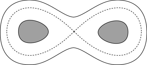
Figure 2: The model system

We compute cohomology using a Čech approach, by choosing an open covering, functions on the sets in the covering, and so on. Although Čech cohomology is defined as the direct limit over the set of all coverings, in ([9], §3) we saw that the interesting features of the cohomology appeared already in the computation using the simplest covering, and so this is what we use here. In §8 we will show that we have computed the actual sheaf cohomology.

Also, by comparison to [18] and [9], we expect the cohomology to only be non-trivial in degree 1, and so from now on when we say “cohomology” without other specification, we mean first cohomology. In section 5.7 we show that other cohomology is trivial.

The simple covering consists of three sets, the “hyperbolic cross” $Z$ together with two other sets covering the rest of $U(\ell)$, as shown in Figure 3:

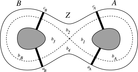
Figure 3: A simple cover of the figure-eight

The thick lines indicate an overlap of open sets, denoted by $AZ$ for $A\cap Z$, etc, and the dotted line indicates the singular leaf. The letters $a$, $b$, and $c$ indicate leafwise flat sections defined on particular sets, the collection of which determines an element of Čech cohomology. We use the convention that $a$ and $c$ are functions on the intersections of two sets, and $b$ are functions on one single set. So, for example, $a_{A}$ is a function defined on $AZ=A\cap Z$, and $b_{A}$ is a function defined on $A$. (Since all overlaps include $Z$, we use $a_{A}$ rather than $a_{AZ}$, for simplicity.) Also, $b^{1}_{Z}$ through $b^{4}_{Z}$ are the sections defined on the quadrants of the hyperbolic cross, making up a leafwise flat section over the cross as in Proposition 11. Thus, the $a$’s and $c$’s make up a Čech 1-cochain, and the $b$’s make up a 0-cochain. Use the ordering convention on the coboundary operator that $(\delta b)$ on $AZ$ is $b_{Z}-b_{A}$, and on $BZ$ is $b_{Z}-b_{B}$.

We are interested in $H^{1}$, and so we are asking: Given $a$’s and $c$’s as in the diagram, which define a 1-cocycle, when do there exist $b$’s so that the coboundary of the $b$ cochain equals the cocycle defined by the $a$’s and $c$’s?

4.1 Parallel transport

In order to compare the values of sections at different points, we use parallel transport.

Given the value of a section at one point $x_{0}$ on a leaf, the value on the rest of the leaf is determined by the condition that the section be leafwise flat. Given a value for $\sigma(x_{0})$, we can construct a leafwise flat $\sigma$ over the entire leaf through $x_{0}$ by parallel transporting $\sigma(x_{0})$ along the leaf.

Given two points $P$ and $Q$ in the same leaf, we will denote parallel transport from $P$ to $Q$ by $\tau_{PQ}$. Thus, if $a$ is a flat section, $a(Q)=a(P)\tau_{PQ}$. Formally, $\tau_{PQ}$ is an automorphism of $\mathbb{L}_{P}$ to $\mathbb{L}_{Q}$; if $\mathbb{L}$ can be trivialized over a set containing both $P$ and $Q$, then we can just think of $\tau_{PQ}$ as a nonzero complex number. Note that $\tau_{PQ}=\tau_{QP}^{-1}$, whether as automorphisms or as complex numbers.

This is related to the description of the sections in Proposition 10 as $a(h)e^{-ih\beta}$. For a fixed value of $h$, say $h_{0}$, once we know $a(h_{0})$, then the value of the section is fixed everywhere on the leaf. The term $e^{-ih\beta}$ represents the change due to parallel transport.

5 Cohomology calculation, part II: explicit calculation

To carry out the computations, we refer to Figure 4.

Figure 4: Diagram for the cohomology calculation

This is the same as Figure 3 with more information: we have added three leaves we will be considering, labelled $\gamma_{1}$, $\gamma_{2}$, and $\gamma_{3}$, and marked points on these leaves as shown. We have also shown the overlaps between sets, so for example $P_{+}$ and $P_{-}$ are in $A\cap Z$.

First, we fix some notation: $\tau^{Z}_{PQ}$ will denote parallel transport from $P$ to $Q$ through the set $Z$. When we are looking at, for example, transport from $P_{+}$ to $Q_{+}$ we will write $\tau^{Z}_{PQ_{+}}$ (rather than $\tau^{Z}_{P_{+}Q_{+}}$). There will never be parallel transport between a “$-$” point and a “$+$” point, because they are on different leaves.

Note that an appropriate combination of parallel transport gives us holonomy: for example,

$$\tau_{PQ_{+}}^{A}\tau_{QP_{+}}^{Z}=\operatorname{hol}_{\gamma_{1}}.$$

Remember that what we are trying to do, exactly, is to answer the following question: Given a collection $\{a_{A},c_{A},a_{B},c_{B}\}$ of sections defining a 1-cochain, when can we find sections $\{b_{A},b_{B},b_{1},b_{2},b_{3},b_{4}\}$ making up a 0-cochain whose coboundary is the given 1-cochain? The set of $a$’s and $c$’s where this is possible gives us $B^{1}$, the set of 1-coboundaries. As it turns out, the three loops $\gamma_{1}$, $\gamma_{2}$, and $\gamma_{3}$ give independent contributions to the cohomology, and $H^{1}(U(\ell);\mathcal{J})$ will be the direct sum of the contributions from each loop. We look at each one in turn and collect the results together in Theorem 18.

5.1 Gamma 1

First look at $\gamma_{1}$. We have the following relations coming from the coboundary conditions:

$$a_{A}(P_{+}) =b_{1}(P_{+})-b_{A}(P_{+})$$ (9a)

$$c_{A}(Q_{+}) =b_{1}(Q_{+})-b_{A}(Q_{+})$$ (9b)

We also have the following relations between the values of the sections at different points:

$$b_{A}(Q_{+}) =b_{A}(P_{+})\tau^{A}_{PQ_{+}}$$ (10a)

$$b_{1}(P_{+}) =b_{1}(Q_{+})\tau^{Z}_{QP_{+}}$$ (10b)

From (10), (9b) becomes

$$c_{A}(Q_{+})=b_{1}(P_{+})(\tau^{Z}_{QP_{+}})^{-1}-b_{A}(P_{+})\tau^{A}_{PQ_{+}}$$

so that the system (9) becomes

$$a_{A}(P_{+}) =b_{1}(P_{+})-b_{A}(P_{+})$$ (11a)

$$c_{A}(Q_{+})\tau^{Z}_{QP_{+}} =b_{1}(P_{+})-b_{A}(P_{+})\tau^{A}_{PQ_{+}}\tau^{Z}_{QP_{+}}$$ (11b)

This can be viewed as a system of two equations for the two unknowns $b_{1}(P_{+})$, $b_{A}(P_{+})$. The coefficient matrix of this system is

$$\begin{bmatrix}1&-1\\ 1&-\tau^{A}_{PQ_{+}}\tau^{Z}_{QP_{+}}\end{bmatrix}$$

which has determinant

$$1-\tau^{A}_{PQ_{+}}\tau^{Z}_{QP_{+}}=1-\operatorname{hol}_{\gamma_{1}}.$$

Thus this matrix is nonsingular, and so (9) has a unique solution, precisely when $\operatorname{hol}_{\gamma_{1}}\neq 1$. This solution is:

$$a_{A}(P_{+})-c_{A}(Q_{+})\tau^{Z}_{QP_{+}}=b_{A}(P_{+})\bigl{(}\operatorname{hol}_{\gamma_{1}}-1\bigr{)}$$ (12a)

$$a_{A}(P_{+})-c_{A}(Q_{+})(\tau^{A}_{PQ_{+}})^{-1}=b_{1}(P_{+})\bigl{(}1-\operatorname{hol}_{\gamma_{1}}\bigr{)}$$ (12b)

This gives $b_{1}$ and $b_{A}$ at the single point $P_{+}$; however, as noted previously, the value of a flat section at one point determines the value everywhere else along the leaf, and so this gives a solution for $b_{A}$ and $b_{1}$ on the entire leaf. Finally, by letting $P_{+}$ vary along a transversal to the leaves, we get $b_{A}$ and $b_{1}$ on the entire neighbourhood inside the singular leaf.

If $\operatorname{hol}_{\gamma_{1}}=1$, then a linear algebra argument shows that (9) has a solution (and thus the cocycle is a coboundary) iff $a_{A}(P_{+})-c_{A}(Q_{+})\tau^{Z}_{QP_{+}}=0$. Since a cocycle is defined by two smooth functions on the transversal (determining the sections $a_{A}$ and $c_{A}$), the Bohr-Sommerfeld contribution to the cohomology from $\gamma_{1}$ is

$$\frac{\{\text{cocycles}\}}{\{\text{coboundaries}\}}\cong\frac{\{(a,c)\text{ smooth functions on an interval}\}}{\{a=c\text{ at one point}\}}$$

This is exactly what we saw appearing in [9] (§3.2.2). As we saw there (Lemma 3.3), the above quotient is isomorphic to $\mathbb{C}$, and so if $\gamma_{1}$ is Bohr-Sommerfeld, it gives a one-dimensional contribution to cohomology. (See also Theorem 18.)

However, this is not the only contribution from $\gamma_{1}$. The flatness properties discussed in §3 affect the calculation as well: in searching for solutions to (9), we do not have complete freedom in choosing $b_{A}$ and $b_{1}$, because of the condition that $b_{1}$ has to be Taylor flat at the singular leaf.

Consider again the system (12). It is valid for all $P_{+}$ inside the singular leaf. If we think of the sections as functions of one variable as $P_{+}$ varies along a transversal to the leaf, then the properties discussed in §3 imply that $b_{1}(P_{+})$, and thus the right-hand side of (12b), is Taylor flat as $P_{+}$ approaches the singular leaf. Therefore, in order for the system (12) to have a solution, it is necessary that

$$a_{A}(P_{+})-c_{A}(Q_{+})(\tau^{A}_{PQ_{+}})^{-1}$$ (13)

be Taylor flat at the singular leaf (viewing $P_{+}$ as a variable, which determines $Q_{+}$), which is to say that $a_{A}$ and $c_{A}(Q_{+})(\tau^{A}_{PQ_{+}})^{-1}$ agree to infinite order at the singular leaf. This will give another contribution in cohomology, which we will clarify in §5.4 and 5.6.

5.2 Gamma 2

The picture is similar for $\gamma_{2}$ as for $\gamma_{1}$. The coboundary equations

$$a_{B}(S_{+}) =b_{3}(S_{+})-b_{B}(S_{+})$$

$$c_{B}(R_{+}) =b_{3}(R_{+})-b_{B}(R_{+})$$

are exactly the same as system (9), with $A$ replaced by $B$, $P$ replaced by $S$, $Q$ replaced by $R$, and $b_{1}$ replaced by $b_{3}$. Thus, they have solutions identical to (12) with these same replacements, namely:

$$a_{B}(S_{+})-c_{B}(R_{+})\tau^{Z}_{RS_{+}} =b_{B}(S_{+})\bigl{(}\operatorname{hol}_{\gamma_{1}}-1\bigr{)}$$ (14)

$$a_{B}(S_{+})-c_{B}(R_{+})(\tau^{B}_{SR_{+}})^{-1} =b_{3}(S_{+})\bigl{(}1-\operatorname{hol}_{\gamma_{1}}\bigr{)}$$ (15)

The second equation gives us, by the same argument, the condition that

$$a_{B}(S_{+})-c_{B}(R_{+})(\tau^{B}_{SR_{+}})^{-1}$$ (16)

has to be Taylor flat at the singular leaf. This gives another “flat functions” contribution to the cohomology, which we will discuss in §5.6.

5.3 Gamma 3

The computation for $\gamma_{3}$ is similar, except that since $\gamma_{3}$ passes through all four components of $AZ$ and $BZ$, we have four equations instead of two. We get a similar phenomenon involving the holonomy, giving us a contribution of $\mathbb{C}$ for each Bohr-Sommerfeld leaf. Since the calculation is similar to (although longer than) the previous two, and since our main interest at the moment is in the flat functions and the infinite contributions to cohomology, we will leave out the Bohr-Sommerfeld calculation, except to note in passing that the Bohr-Sommerfeld contribution will come from the holonomy all around $\gamma_{3}$, but will still give one factor of $\mathbb{C}$ in cohomology. Thus, the Bohr-Sommerfeld leaves inside and outside the singular leaf make equal contributions to the cohomology. For example, in the torus realization mentioned in section 4, even if the level set has two connected components (represented in Figure 2 by the inner circles), each component is independent in terms of its cohomology. (In fact, since these leaves are regular, Śniatycki’s results apply to give us their contribution to cohomology directly.)

We focus now on the question of role of the flat functions for $\gamma_{3}$. As there are two Taylor flat functions in this computation, $b_{4}$ and $b_{2}$, we wish to find the solutions to the coboundary equations for $b_{4}$ and $b_{2}$, which will give us two conditions that certain combinations of the $a$’s and $c$’s have to be Taylor flat. The calculations are similar in form, though more complicated, to those given in 5.1. Out of compassion for the reader, we omit the details, and merely give the results.

We start with four equations coming from the coboundary conditions, starting at $P_{-}$:

$$a_{A}(P_{-}) =b_{4}(P_{-})-b_{A}(P_{-})$$ (17a)

$$c_{A}(Q_{-}) =b_{2}(Q_{-})-b_{A}(Q_{-})$$ (17b)

$$c_{B}(R_{-}) =b_{2}(R_{-})-b_{B}(R_{-})$$ (17c)

$$a_{B}(S_{-}) =b_{4}(S_{-})-b_{B}(S_{-})$$ (17d)

We also have relationships between the values of each function at different points, coming from parallel transport:

$$b_{A}(Q_{-}) =b_{A}(P_{-})\tau^{A}_{PQ_{-}}$$ (18a)

$$b_{2}(R_{-}) =b_{2}(Q_{-})\tau^{Z}_{QR_{-}}$$ (18b)

$$b_{B}(S_{-}) =b_{B}(R_{-})\tau^{B}_{RS_{-}}$$ (18c)

$$b_{4}(P_{-}) =b_{4}(S_{-})\tau^{Z}_{SP_{-}}$$ (18d)

Starting at $P_{-}$, we can use these formulae to “push along” the leaf until we come back around to $P_{-}$. The calculation involving $b_{4}$ (details omitted) yields

$$b_{4}(P_{-})-b_{4}(P_{-})\tau^{A}_{PQ_{-}}\tau^{Z}_{QR_{-}}\tau^{B}_{RS_{-}}\tau^{Z}_{SP_{-}}=a_{B}(S_{-})\tau^{Z}_{SP_{-}}\\ +c_{A}(Q_{-})\tau^{Z}_{QR_{-}}\tau^{B}_{RS_{-}}\tau^{Z}_{SP_{-}}-a_{A}(P_{-})\tau^{A}_{PQ_{-}}\tau^{Z}_{QR_{-}}\tau^{B}_{RS_{-}}\tau^{Z}_{SP_{-}}-c_{B}(R_{-})\tau^{B}_{RS_{-}}\tau^{Z}_{SP_{-}}$$ (19)

We recognize the coefficient of the second $b_{4}$ as the holonomy (it also appears with $a_{A}$), and so this simplifies to

$$\begin{split}b_{4}(P_{-})\bigl{(}1-\operatorname{hol}_{\gamma_{3}}\bigr{)}=a_{B}(S_{-})\tau^{Z}_{SP_{-}}+c_{A}(Q_{-})\tau^{Z}_{QR_{-}}\tau^{B}_{RS_{-}}\tau^{Z}_{SP_{-}}\\ -a_{A}(P_{-})\operatorname{hol}_{\gamma_{3}}-c_{B}(R_{-})\tau^{B}_{RS_{-}}\tau^{Z}_{SP_{-}}.\end{split}$$ (20)

As in the previous sections, this tells us that this particular combination of $a$’s and $c$’s has to be Taylor flat at the singular leaf in order for the cohomology equations to have a solution.

At first, this seems like another condition, which will give another contribution to the cohomology. However, if we look more closely, we see that it is not independent of our earlier conditions. Explicitly, if we take (13) times $\operatorname{hol}_{\gamma_{3}}$ plus (16) times $-\tau^{Z}_{SP_{+}}$, we obtain exactly the right-hand side of (20), except the points have $+$’s instead of $-$’s. However, the condition applies at the singular leaf. Since $P_{+}$ and $P_{-}$ approach the same point on the singular leaf, and since the Taylor series of a function is the same “from either side,” the condition in (20) is already implied by conditions coming from (12) and (14), and so does not give any new contribution to the cohomology.

Similarly, we can go through the same process to solve (17) for $b_{2}$, which gives us another combination of $a$s and $c$s that has to be Taylor flat at the singular leaf, but which also turns out to be already implied by (12) and (14).

5.4 The “flat functions” contribution to cohomology

So far we have found two independent conditions (13) and (16) that certain combinations of sections must be analytically flat (as well as two similar conditions that turn out not to be independent). In this section we explore what contributions these conditions make to the cohomology. In both cases, the condition requires that two sections agree to infinite order at the singular leaf, which is equivalent to the condition that two functions of one variable (on a transversal to the leaf, defining the section) agree to infinite order at one point. Let $I$ be an open interval, and fix a reference point $x_{0}\in I$. For two functions $a,c\in C^{\infty}(I)$, let $a\approx c$ mean that $a$ and $c$ agree to infinite order at $x_{0}$. Since each section is defined by a function on a transversal to the leaves, and the coboundaries are those where the two functions agree to infinite order at the singular leaf, we will be looking at quotients of the form $C^{\infty}(I)^{2}/\{a\approx c\}$.

Lemma 17.

The quotient $C^{\infty}(I)^{2}/\{a\approx c\}$ is isomorphic to the space of complex-valued sequences, which we denote by $\mathbb{C}^{\mathbb{N}}$.

Proof.

Let $a^{(n)}(x_{0})$ denote the $n^{\text{th}}$ Taylor coefficient of $a$ at $x_{0}$. Then map $C^{\infty}(I)^{2}$ to $\mathbb{C}^{\mathbb{N}}$ by the map that puts $\bigl{(}a^{(n)}(x_{0})-c^{(n)}(x_{0})\bigr{)}$ in the $n^{\text{th}}$ place. This map has kernel exactly $\{a\approx c\}$. To see it is surjective we apply Borel’s theorem which says that given a sequence $z_{n}$ of complex numbers there exists a complex smooth function $f$ such that $f^{(p)}(x_{0})=z_{p}$. (See for example [20] or [16].) ∎

5.5 If the singular leaf is Bohr-Sommerfeld

So far, we have only considered the possibility of non-singular Bohr-Sommerfeld leaves. What happens if the singular leaf is Bohr-Sommerfeld? (Note that each of the two loops in the singular leaf can be Bohr-Sommerfeld, and that these conditions are independent.)

Look at the system (12), which we reproduce here, and consider what happens as $\gamma_{1}$ approaches the singular leaf.

$$a_{A}(P_{+})-c_{A}(Q_{+})\tau^{Z}_{QP_{+}}=b_{A}(P_{+})\bigl{(}\operatorname{hol}_{\gamma_{1}}-1\bigr{)}$$

$$a_{A}(P_{+})-c_{A}(Q_{+})(\tau^{A}_{PQ_{+}})^{-1}=b_{1}(P_{+})\bigl{(}1-\operatorname{hol}_{\gamma_{1}}\bigr{)}$$

The holonomy $\operatorname{hol}_{\gamma_{1}}$ will be a smooth function of the “leaf variable,” and so we can look at each side of, say, the first equation above as a function of the “leaf variable.” Even if the holonomy at the singular leaf is 1, so that the right side vanishes at the singular leaf, the right side as a function already vanishes to infinite order at the singular leaf. Thus the left side still has to be Taylor flat, and so we still get the infinite-dimensional contribution to cohomology, regardless of whether the singular leaf is Bohr-Sommerfeld or not.

On the other hand, the contribution of one factor of $\mathbb{C}$ for a regular Bohr-Sommerfeld leaf does not occur for the singular leaf. This factor comes out of the cohomology calculation because of a condition that the values of $a$ and $c$ at the Bohr-Sommerfeld leaf have to agree, but this is already required by the condition that they have to agree to infinite order. Thus there is no additional Bohr-Sommerfeld contribution.

5.6 Summary of the calculations

Here we collect the results from the preceding calculations into one place.

Theorem 18.

The first cohomology of the neighbourhood $U(\ell)$ of the figure-eight hyperbolic system given in Figure 2 has two contributions of the form $\mathbb{C}^{\mathbb{N}}$, each one corresponding to a space of Taylor series in a complex variable. It also has one $\mathbb{C}$ term for each non-singular Bohr-Sommerfeld leaf. That is,

$$H^{1}\bigl{(}U(\ell),\mathcal{J}\bigr{)}\cong\mathbb{C}^{\mathbb{N}}\oplus\mathbb{C}^{\mathbb{N}}\oplus\bigoplus_{b\in BS}\mathbb{C}_{b}$$ (21)

where the sum is over the non-singular Bohr-Sommerfeld leaves.

Proof.

Let the points $P$, $Q$, $R$ and $S$ be the points on the singular leaf that are the limits of $P_{+}$, $P_{-}$, $Q_{+}$,$Q_{-}$, etc. when $\gamma_{1}$, $\gamma_{2}$ and $\gamma_{3}$ approach the singular leaf. As we pointed out in the computations involving $\gamma_{1}$ and $\gamma_{2}$, the expressions

$$a_{A}(P_{+})-c_{A}(Q_{+})(\tau^{A}_{PQ_{+}})^{-1}$$

(equation (13)) and

$$a_{B}(S_{+})-c_{B}(R_{+})(\tau^{B}_{SR_{+}})^{-1}$$

(equation (16)) can be seen as functions in the variables $P_{+}$ and $S_{+}$ respectively (since the variables $Q_{+}$ and $R_{+}$ can be determined from these). These functions can be seen as functions on the two transversals at $P$ and $S$ to the singular leaf. Thus we can think of these functions as functions of one variable (on an open interval $I$ centered at zero), which we denote by $a_{A}-c_{A}\tau^{A}$ and $a_{B}-c_{B}\tau^{B}$, respectively. As in Lemma 17, let $f^{(n)}(0)$ denote the $n^{\text{th}}$ Taylor coefficient of the function $f$ at $0$.

As noted at the beginning of §5, the space $Z^{1}$ of 1-cocycles is the collection $Z^{1}=\{(a_{A},c_{A},a_{B},c_{B})\}$. Map $Z^{1}$ into the right-hand side of (21) as follows:

• Map $(c_{A},a_{A},c_{B},a_{B})$ to $(a_{A}-c_{A}\tau^{A})^{(n)}(0)$ in the $n^{\text{th}}$ term of the first $\mathbb{C}^{\mathbb{N}}$ factor, and

• $(c_{A},a_{A},c_{B},a_{B})$ to $(a_{B}-c_{B}\tau^{B})^{(n)}(0)$ in the $n^{\text{th}}$ term of the second $\mathbb{C}^{\mathbb{N}}$ factor; also,

• for each non-singular Bohr-Sommerfeld leaf, passing through points $P_{j}$ and $Q_{j}$, map $(a_{A},c_{A},a_{B},c_{B})$ to $a_{A}(P_{j})-c_{A}(Q_{j})\tau^{Z}_{Q_{j}P_{j}}$ in the $\mathbb{C}$ component corresponding to that Bohr-Sommerfeld leaf.

From the preceding discussion, the kernel of this map is precisely the set of coboundaries, as follows. From §5.1, if the cocycle is a coboundary then $a_{A}-c_{A}\tau_{A}$ is Taylor flat at the singular leaf (equation (13)). From §5.2, (16), we have the same for $a_{B}-c_{B}\tau^{B}$. And finally, for each regular Bohr-Sommerfeld leaf, being a coboundary requires that the values of the corresponding $a$ and $c\tau$ functions agree on that leaf. Conversely, if all these conditions hold, the collection $(c_{A},a_{A},c_{B},a_{B})$ defines a coboundary. Thus, the kernel of this map is the set of coboundaries.

On the $\mathbb{C}^{\mathbb{N}}$ components, this map is the same map as was used in the proof of Lemma 17, which was shown there to be surjective, and so this map is surjective onto the $\mathbb{C}^{\mathbb{N}}$ components. It is also surjective on the $\mathbb{C}$ components: the $(a-c\tau)^{(n)}(0)$ determine the jet of the functions at the origin, but not their values at any point away from the origin. Since $a_{A},c_{A}$, etc. can be any smooth functions, it is easy to choose them so that $a_{A}(P_{j})-c_{A}(Q_{j})\tau_{P_{j}Q_{j}}$ has any desired value. Thus, the map is surjective onto the $\mathbb{C}$ components.

Finally, if the singular leaf is Bohr-Sommerfeld, it is excluded from the sum by §5.5.

Therefore we have a surjective map from the space of cocycles to the right side of (21) whose kernel is the space of coboundaries, and so the cohomology is as claimed. ∎

Remark 19.

We can make the infinite-dimensional cohomology look slightly more natural by viewing it as a graded vector space. Following the ideas of the Arnol’d school around singularity theory (see for example [1]), it is possible to define a filtration on the sheaf $\mathcal{J}$ by letting $\mathcal{J}_{k}$ consist of solutions up to order $k$ of the leafwise flat sections equation. This induces a grading on the cohomology, so that the $\mathbb{C}^{\mathbb{N}}$ term has one $\mathbb{C}$ in each degree.

5.7 Cohomology in other degrees

So far we have been concerned with the cohomology in degree 1. We now briefly dispose of the other degrees.

Theorem 20.

Let $(U(\ell),\omega,F)$, $\mathbb{L}$, and $\mathcal{J}$ be as above. Then the cohomology groups $H^{k}\bigl{(}U(\ell),\mathcal{J}\bigr{)}$ are zero for $k\neq 1$.

Proof.

This is immediate. First, $H^{0}\bigl{(}U(\ell),\mathcal{J}\bigr{)}$ is the set of global leafwise flat sections of $\mathbb{L}$. Any such section is zero except on the Bohr-Sommerfeld leaves; since the set of Bohr-Sommerfeld leaves is discrete, the entire section must be zero by continuity, and so $H^{0}\bigl{(}U(\ell),\mathcal{J}\bigr{)}=0$. Higher cohomology groups are trivial because there are no triple or higher intersections in the cover. ∎

Remark.

Although we have computed the cohomology with respect to a certain cover (and this is particularly evident here), we show in §8 that it is isomorphic to the actual sheaf cohomology.

6 More than one singular point

Thus far, all of the calculations have been for the simplest system with a hyperbolic singularity, given in Figure 2. In this section we perform the calculations for more complicated systems.

6.1 The next simplest examples

In the case where there is more than one hyperbolic singular point on the same leaf, there are many different possibilities for the topology of the leaf. Two examples are the “triple-eight” with three loops and the “double-lung” systems, each with two hyperbolic singularities, shown below in Figures 5 and 6. Bolsinov and Fomenko in [2] give a classification of the possible topological types of leaves.

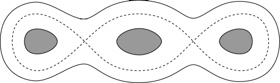
Figure 5: The “triple-eight” system

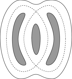
Figure 6: The “double-lung” system

We first consider the “triple-eight” and carry out the cohomology calculation for this system. Loops around either of the two outside “holes,” inside the singular leaf, will clearly give identical calculations as in the figure-eight case, and so we do not repeat them. The computation for the middle loop $\gamma_{4}$, shown in Figure 7, is a bit different.

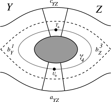
Figure 7: Closeup of the centre loop

From $YZ$ we get the two equations

$$a_{YZ}(T_{+})=b_{Z}^{3}(T)-b_{Y}^{1}(T)$$ (22a)

$$c_{YZ}(U)=b_{Z}^{3}(U)-b_{Y}^{1}(U)$$ (22b)

and from parallel transport we get

$$b_{Z}^{3}(U)=b_{Z}^{3}(T)\tau^{Z}_{TU}$$ (23a)

$$b_{Y}^{1}(T)=b_{Y}^{1}(U)\tau^{Y}_{UT}$$ (23b)

Use (23) to write (22b) at $T$:

$$c_{YZ}(U)=b_{Z}^{3}(T)\tau^{Z}_{TU}-b_{Y}^{1}(T)\tau^{Y}_{TU}$$

so

$$c_{YZ}(U)\tau^{Y}_{UT}=b_{Z}^{3}(T)\tau^{Z}_{TU}\tau^{Y}_{UT}-b_{Y}^{1}(T)$$

Subtracting this from (22a), we get

$$\begin{split}a_{YZ}(T)-c_{YZ}(U)\tau^{Y}_{UT}&=b_{Z}^{3}(T)-b_{Y}^{1}(T)-b_{Z}^{3}(T)\tau^{Z}_{TU}\tau^{Y}_{UT}+b_{Y}^{1}(T)\\ &=b_{Z}^{3}(T)\bigl{(}1-\operatorname{hol}_{\gamma_{4}}\bigr{)}\end{split}$$ (24)

A similar procedure gives us a solution for $b^{1}_{Y}$ in terms of $a_{YZ}$ and $c_{YZ}$, also involving a holonomy term. These are the familiar equations involving holonomy, which give us the contribution due to a Bohr-Sommerfeld leaf.

However, the more interesting part is the contribution coming from flat functions, for which we don’t even need the calculation leading to (24), but we can see directly from (22). Since $b_{Y}^{1}$ and $b_{Z}^{3}$ are both Taylor flat at the singular leaf, the right-hand sides of (22a) and (22b) both vanish to infinite order at the singular leaf, and so in order for (22) to have a solution, it is necessary that both $a_{YZ}$ and $c_{YZ}$ vanish to infinite order at the singular leaf as well. Thus, this piece gives a contribution to the cohomology that looks like

$$\{\text{smooth functions}\}^{2}/\{a\approx 0,\,c\approx 0\}$$

namely, $(\mathbb{C}^{\mathbb{N}})^{2}$. Together with the two contributions coming from the loops around the outer “holes,” each of which will be one contribution of $\mathbb{C}^{\mathbb{N}}$, we see that there are a total of four $\mathbb{C}^{\mathbb{N}}$ contributions from the pair of singularities.

We leave as an exercise for the reader to set up and carry out the computations for the “double lung” system in Figure 6, and show that it also has four $\mathbb{C}^{\mathbb{N}}$ components in the cohomology.

6.2 The general case

Here we show that, in general, we get two $\mathbb{C}^{\mathbb{N}}$ contributions to the cohomology for each hyperbolic singular point.

Consider a covering of a neighbourhood of the singular leaf by overlapping rectangles together with hyperbolic crosses, as illustrated in Figure 8 (and as used in §8). Near a hyperbolic singular point, the system looks like Figure 9.

Figure 8: The covering of the leaf

Figure 9: The covering near one hyperbolic singular point

Consider the part of the leaf passing through the set labelled $A$ in Figure 9. If we continue along this leaf, we will pass through a number of other rectangles, each with their own functions defined on them and on the corresponding intersections, and eventually reach another hyperbolic cross (possibly the same one on a different branch). See Figure 10, where the $a$’s denote elements of $\mathcal{J}$ on double intersections (part of a 1-cochain), and the $b$’s denote elements on the sets (part of a 0-cochain).

Figure 10: Leaf between two singular points

If we look at the coboundary conditions for this part of the picture, we will get a system of equations like

$$\begin{split}a_{1}&=b_{1}-b_{Z}\\ a_{2}&=b_{2}-b_{1}\\ &\vdots\\ a_{n}&=b_{Y}-b_{n-1}\end{split}$$ (25)

(where for simplicity we have omitted the terms giving parallel transport). Adding up all these equations gives

$$a_{1}+a_{2}+\cdots+a_{n}=b_{Y}-b_{Z}$$ (26)

which, since $b_{Y}$ and $b_{Z}$ must be analytically flat, shows that the sum of the $a_{j}$’s must be analytically flat.

The part of the cohomology coming from this part of the picture will therefore have a term of the form

$$\frac{C^{\infty}(I)^{\oplus n}}{\{a_{1}+\cdots+a_{n}\approx 0\}},$$ (27)

which is isomorphic to $\mathbb{C}^{\mathbb{N}}$ by a similar argument as in the proof of Lemma 17. Thus, the $H^{1}$ cohomology will have one term of the form $\mathbb{C}^{\mathbb{N}}$ coming from this part of the singular leaf.

This will be true for each arc connecting two singularities in the singular leaf, and these conditions will be independent of each other. Since there are twice as many such arcs as singular points (four emitting from each point, each of which gets counted twice this way), there are two $\mathbb{C}^{\mathbb{N}}$ contributions in per singularity.

For the same reason as in the proof of Theorem 20 (namely that the covering has no triple or higher intersections), the higher cohomology groups are zero. From [9], we have a Mayer-Vietoris principle for this cohomology (see Propositions 3.4.2 and 6.3.1). Putting together the results of this section with the results from [18] and [9] (which give the regular and elliptic cases, respectively), and patching together with Mayer-Vietoris, we obtain the following:

Theorem 21.

Let $(M,\omega,F)$ be a two-dimensional, compact, completely integrable system, whose moment map has only nondegenerate singularities. Suppose $M$ has a prequantum line bundle $\mathbb{L}$, and let $\mathcal{J}$ be the sheaf of sections of $\mathbb{L}$ flat along the leaves. The cohomology $H^{1}(M,\mathcal{J})$ has two contributions of the form $\mathbb{C}^{\mathbb{N}}$ for each hyperbolic singularity, each one corresponding to a space of Taylor series in one complex variable, and one $\mathbb{C}$ term for each non-singular Bohr-Sommerfeld leaf. That is,

$$H^{1}(M;\mathcal{J})\cong\bigoplus_{p\in\mathcal{H}}\bigl{(}\mathbb{C}^{\mathbb{N}}\oplus\mathbb{C}^{\mathbb{N}}\bigr{)}\oplus\bigoplus_{b\in BS}\mathbb{C}_{b}.$$ (28)

The cohomology in other degrees is zero.

Thus in particular, the quantization of $M$ is given by (28).

Remark.

So far, we have only shown the above for cohomology computed with respect to the particular coverings used in the computations, but we prove below in §8 that this is isomorphic to the actual sheaf cohomology.

7 Dependence on polarizations

The theorem above establishes a strong dependence of the quantization of an integrable system on a surface on the singularities of the function determining the integrable system. In particular, if we can find examples of integrable systems on the same surface with different kinds of singularities, Theorem 21 would show that this notion of quantization depends strongly on the polarization considered.

7.1 Two examples from Mechanics

In this section we give two examples which show up naturally in mechanics and then we give a method to construct general examples of surfaces with prescribed number of hyperbolic singularities.

Example 1: Rotations on the sphere

Consider the height function $h$ on the 2-sphere of integer height $k$ together with its standard area form. The Hamiltonian vector field of the function $h$ is the vector field given by rotations along the central axis.

As described in [9] Chapter 5, this system has $k-1$ non-singular Bohr-Sommerfeld leaves, corresponding to the circles with integer height. A picture of the integrable system with the Bohr-Sommerfeld leaves marked on it for $k=4$ is shown in Figure 11.

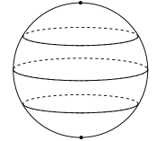
Figure 11: The height function on a sphere

According to theorem 21, the dimension of the quantization for this integrable system is just given by the regular Bohr-Sommerfeld leaves, which in this case is $k-1$. The elliptic singularities (north and south poles) do not contribute.

Example 2: Euler’s equations restricted to a sphere

Consider Euler’s equations of the rigid body on $T^{*}(SO(3))$ and consider the lifted action of $SO(3)$. These equations correspond to the movement of the Euler top (a rigid body moving around its center of mass) which has configuration space $SO(3)$. Using symplectic reduction by the lifted action of $SO(3)$ we obtain a Hamiltonian system on $S^{2}$. The topology and geometry of the induced system on the symplectic reduced space is well-known; see for example Cushman and Bates [3] for details. In section III.4, they show that this system has two hyperbolic singularities and four elliptic singularities.

A picture of the integrable system is given in Figure 12.

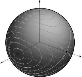
Figure 12: Reduced Hamiltonian flow of Euler’s equations

Using the recipe given in Theorem 21, the quantization of this system is

$$\mathcal{Q}(M)=H^{1}(M;\mathcal{J})\cong\bigoplus_{p\in\mathcal{H}}(\mathbb{C}_{p}^{\mathbb{N}})^{2}\oplus\bigoplus_{b\in BS}\mathbb{C}_{b}.$$

Since the hyperbolic set has two elements, this cohomology group has four infinite-dimensional contributions. If we compare this example to the previous one (in which the quantization is finite-dimensional), we can conclude that this quantization of the sphere strongly depends on the polarization when we allow singularities.

7.2 Surgery of integrable systems

Indeed, we can perform surgery of integrable systems to include as many hyperbolic singularities into the picture as the Euler characteristic allows. We briefly present this method in this small subsection, for the sake of completeness. Though the construction might seem elementary, such an explicit description is not detailed in the literature of integrable systems.

Given a function on a compact orientable surface $f\colon S\longrightarrow\mathbb{R}$ with non-degenerate singularities (a Morse function), consider the Hamiltonian vector field $X_{f}$ associated to this function. It is well-known (see for instance, [13]) that the number of elliptic and hyperbolic singularities of this vector field on a surface is related to the Euler characteristic via the Poincaré-Hopf formula:

$$\chi(S)=\text{number of elliptic singularities}-\text{number of hyperbolic singularities}$$ (29)

In the case of compact orientable surfaces, we can find examples of integrable systems on them with any numbers $s_{e}$ of elliptic and $s_{h}$ hyperbolic singularities greater than for the height function and satisfying (29). These examples can be created via surgery of integrable systems, adding cylinders with one elliptic and one hyperbolic singularity and therefore increasing by one the number of each type of singularity at each step. Bolsinov and Fomenko [2] have developed a whole Morse theory for integrable systems of singularities with special attention to the cases of surfaces.

We denote $s_{e}^{0}$ and $s_{h}^{0}$ the total number of elliptic and hyperbolic singularities given by the height function on the compact surface.

The method has the following steps, which we illustrate on the sphere in the figures below.

Step 1: Start with the height function $h$ on a given compact surface. Cut out a cylinder containing only regular levels following the level sets of the height function $h$. The upper and lower border of the cylinder are level sets of $h$. (Figure 13)

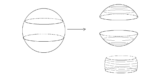
Figure 13: Cutting out a cylinder.

Step 2: Leaving the foliation by level sets of $h$ the same on the complement of the cylinder, change the function inside the cylinder (which is regular) in such a way as to create a hyperbolic singularity and simultaneously an elliptic singularity inside the cylinder. See Figure 14.

   

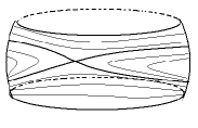
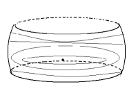
Figure 14: Hyperbolic singularity inside the cylinder. (Front and rear view)

Step 3: Glue the cylinder back into the surface. This gives an example of a “modified” integrable system with one more elliptic and one more hyperbolic singularity than we started with.

Finally, given $s_{e}$ and $s_{h}$ such that $\chi(S)=s_{e}-s_{h}$ and $s_{e}\geq s_{e}^{0}$ and $s_{h}\geq s_{h}^{0}$, by repeating this process we can obtain an example of an integrable system on a compact surface with exactly $s_{e}$ elliptic singularities and $s_{h}$ hyperbolic singularities.

For these systems, we can apply the main recipe of theorem 21 to get the following result:

Proposition 22.

The quantization of the integrable system constructed above via integrable surgery on a compact orientable surface with Euler characteristic $\chi(S)=s_{e}-s_{h}$ and exactly $s_{e}$ elliptic and $s_{h}$ hyperbolic singularities such that $s_{e}\geq s_{e}^{0}$ and $s_{h}\geq s_{h}^{0}$ is given by the formula:

$$H^{1}(M;\mathcal{J})\cong\mathbb{(}C^{\mathbb{N}})^{2s_{h}}\oplus\bigoplus_{b\in BS}\mathbb{C}_{b}.$$

This shows that this quantization of any compact surface strongly depends on the polarization when we allow polarizations with singularities.

8 Refinements and coverings

In this somewhat technical section we show that the cohomology computed in sections 4 – 6 is the actual sheaf cohomology. We use the methods and terminology of [9], especially §3.4 and 3.5. We review these briefly and refer the reader there for more details.

Let $M$ be a compact 2-dimensional prequantized integrable system, as usual. Recall that sheaf cohomology is defined as the direct limit, over all open coverings of $M$, of the cohomology computed with respect to the cover. In order to show that the cohomology we have computed in §5 is the actual sheaf cohomology, we show that every open covering has a refinement whose cohomology is isomorphic to that found in §5. For simplicity, we assume that $M$ has only one leaf with hyperbolic singularities; the extension to the case of several such leaves is reasonably straightforward.

We copy from [9] the following definition. We assume we have a given set of coordinates (which will usually be action-angle coordinates), which we call $(t,\theta)$.

Definition 23.

A brick wall cover of a $t$-$\theta$ rectangle is a finite covering by open $t$-$\theta$ rectangles (“bricks”), satisfying the following properties:

• The rectangles can be partitioned into sets (“layers”) so that all rectangles in one layer cover the same interval of $t$ values (“All bricks in the same layer have the same height”);

• Each brick contains points that are not in any other brick; and

• There are no worse than triple intersections, i.e., the intersection of two bricks in one layer does not meet the intersection of two bricks in either of the two adjoining layers.

    

Figure 15: A brick wall cover, and one which is not

Note that we do not require that the number of bricks be the same in each layer, nor that the layers have the same height, nor that the bricks within one layer have the same width. See Figure 15, where thick lines indicate intersections. The definition extends in the obvious way to cylinders, where we identify $\theta=0$ and $\theta=2\pi$.

Let $\mathfrak{U}$ be an open covering of $M$. By Lebesgue’s number lemma, there is some number $\delta$ such that any set of diameter less than $\delta$ is contained entirely in some set $U\in\mathfrak{U}$.

Let $L_{\delta}$ be a “fattening” of the singular leaf, a neighbourhood of the singular leaf which is the union of leaves of width $\delta/2$. Cover $L_{\delta}$ by rectangles of width $\delta/2$, together with a small “hyperbolic cross” at the singularity that also has diameter less than $\delta$. Then let the open covering $\mathfrak{V}$ be the collection of these rectangles, together with a brick wall covering of $M\smallsetminus L_{\delta}$ with bricks of diameter less than $\delta$. Then $\mathfrak{V}$ is a refinement of $\mathfrak{U}$.

Now we show that the Čech cohomology of $M$ calculated with respect to $\mathfrak{V}$ is the same as we found in 5.

Let $E$ be the union of all layers of bricks which do not meet the singular leaf. Let $A\subset L_{\delta}$ be an open union of leaves around the singular leaf which does not intersect $E$ and which does not contain any Bohr-Sommerfeld leaf other than possibly the singular leaf. (This is possible by the discreteness of Bohr-Sommerfeld leaves.) Let $B$ be an open union of regular leaves such that $A\cup B=M$. Then the covering $\mathfrak{V}$ induces a covering on $A$ and $B$ which is a brick wall covering on $B$, and on $A$ has the same form as shown in Figure 8.

(The point of this construction is the following: $A$ meets only one layer of bricks, namely the ones covering the singular leaf. $B$ is an open union of leaves which, together with $A$, covers $M$. We have chosen $A$ and $B$ so that all intersections between layers of bricks happen outside of $A$. This means that the covering induced on $A$ has no triple intersections, and we can apply the results of §6.2. Since we have from [9] a Mayer-Vietoris for unions of regular leaves, and since $A\cap B$ consists only of regular leaves, we can apply Mayer-Vietoris to $A$ and $B$. Thus we avoid having to calculate with a covering of $A$ with more “layers of bricks,” and thus avoid triple intersections.)

By the assumption that $A$ contains no Bohr-Sommerfeld leaf, the cohomology of $A$ with respect to the covering induced by $\mathfrak{V}$ is $\mathbb{C}^{2\mathbb{N}}$ in degree 1, and zero otherwise. Since $B$ is regular, the results of [9] apply, and the cohomology of $B$ with respect to the covering induced by $\mathfrak{V}$ has one dimension for every (nonsingular) Bohr-Sommerfeld leaf.

By Mayer-Vietoris, $H^{*}_{\mathfrak{V}}(M)\cong H^{*}_{\mathfrak{V}}(A)\oplus H^{*}_{\mathfrak{V}}(B)$ since $A\cap B$ is regular and has no Bohr-Sommerfeld leaves.

Therefore, the cohomology of $M$ calculated with respect to the covering $\mathfrak{V}$ is the same as that calculated with respect to the covering in §4.

Since every open covering $\mathfrak{U}$ has a refinement of the form $\mathfrak{V}$, we have computed the actual sheaf cohomology of $M$.

References

- [1] V. I. Arnold, S.M. Gusein-Zade and A.N. Varchenko, Singularities of Differentiable Maps: Volumes 1 and 2. Monographs in Mathematics, Birkhauser, 1988.
- [2] A. V. Bolsinov and A. T. Fomenko, Integrable Hamiltonian systems: geometry, topology, classification, Chapman & Hall/CRC, 2004.
- [3] R. H. Cushman and L. M. Bates. Global aspects of classical integrable systems. Birkhäuser Verlag, Basel, 1997.
- [4] Y. Colin de Verdi re and J. Vey, Le lemme de Morse isochore. Topology 18 (1979), no. 4, 283–293.
- [5] L. H. Eliasson, Normal forms for Hamiltonian systems with Poisson commuting integrals, Ph.D. Thesis (1984).
- [6] J.P. Dufour, P. Molino and A. Toulet, Classification des systèmes intégrables en dimension et invariants des modèles de Fomenko. C. R. Acad. Sci. Paris Sér. I Math. 318 (1994), no. 10, 949–952.
- [7] L. H. Eliasson, Normal forms for Hamiltonian systems with Poisson commuting integrals—elliptic case, Comment. Math. Helv. 65 (1990), no. 1, 4–35.
- [8] V. Guillemin and S. Sternberg. The Gel’fand-Cetlin system and quantization of the complex flag manifolds. J. Funct. Anal., 52(1):106–128, 1983.
- [9] M. Hamilton, “Locally toric manifolds and singular Bohr-Sommerfeld leaves,” to appear in Mem. AMS, http://arxiv.org/abs/0709.4058
- [10] V. Ginzburg, V. Guillemin and Y. Karshon, Moment maps, cobordisms, and Hamiltonian group actions, AMS Monographs, 2004.
- [11] B. Kostant, “On the Definition of Quantization,” Geometrie Symplectique et Physique Mathematique, Coll. CNRS, No. 237, Paris, (1975), 187-210.
- [12] J. Marsden, T. Ratiu, Introduction to mechanics and symmetry: A basic exposition of classical mechanical systems, Second edition. Texts in Applied Mathematics, 17. Springer-Verlag, New York, 1999.
- [13] J. Milnor, Morse theory, Princeton University, 1963
- [14] E. Miranda and San Vu Ngoc, ”A singular Poincaré lemma”, IMRN,1, 27-46, (2005).
- [15] E. Miranda, On symplectic linearization of singular Lagrangian foliations, Ph.D. Thesis, Univ. de Barcelona, 2003.
- [16] H.-J. Petzsche, “On E. Borel’s Theorem” Math. Ann. 282, 299-313 (1988)
- [17] J. Rawnsley, ” On the Cohomology Groups of a Polarization and Diagonal quantization”, Transaction of the American Mathematical Society, Vol 230 (1977) pp 235-255
- [18] J. Śniatycki, “On Cohomology Groups Appearing in Geometric Quantization”, Differential Geometric Methods in Mathematical Physics I (1975)
- [19] J. Śniatycki, Geometric quantization and quantum mechanics. Applied Mathematical Sciences, 30. Springer-Verlag, New York-Berlin, 1980.
- [20] J.C. Tougeron, Idéaux de fonctions différentiables, Ergebnisse der Mathematik und ihrer Grenzgebiete, Band 71, Springer-Verlag, Berlin-New York, 1972. vii+219 pp
- [21] J. Williamson, On the algebraic problem concerning the normal forms of linear dynamical systems, Amer. J. Math. 58:1 (1936), 141-163.
- [22] N.M.J. Woodhouse, Geometric quantization, Second edition. Oxford Mathematical Monographs, Oxford Science Publications, The Clarendon Press, Oxford University Press, New York, 1992.