Geometric Phase and Quantum Phase Transition : Two-Band Model

Abstract

The connection between the geometric phase and quantum phase transition has been discussed extensively in the two-band model. By introducing the twist operator, the geometric phase can be defined by calculating its ground-state expectation value. In contrast to the previous numerical examinations, our discussion presents an exact calculation for the determination of the geometric phase. Through two representative examples, our calculation shows the intimate connection between the geometric phase and phase transition: different behaviors of the geometric phase can be identified in this paper, which are directly related to the energy gap above the ground state.

I introduction

Recently, quantum phase transition sachdev has received great attention due to its intimate correlation to the fundamental principles of quantum mechanics, especially to the concept of quantum entanglement preskill ; osterloh ; wu ; vidal ( see Ref.afov07 for a comprehensive review ). In general the quantum phase transition happens when the degeneracy of the ground states occurs, which cannot be characterized completely by the pattern of symmetry broken ( order parameters of some kind ). Instead the universal quantum order or topological order is needed for the description of properties of the ground state in many-body systems wen . Recently the connection between the geometric phase of the ground state and the quantum criticality has been displayed in spin-chain systems by displaying the singularity of the geometric phase closed to the critical points carollo ; zhu . Moreover in Ref zhu the author showed that the scaling behavior of the geometric phase of the ground state near the critical points can also display the universal class of the phase transitions. Many works have been devoted to this interesting issue cui ; rhp07 ; Zanardi ; pv ( or see Ref.zhu08 for a review ).

Although great progresses has been made in the understanding of quantum phase transition from the fundamental principles of quantum mechanics, an important question is not yet resolved: whether there exists a universal way to characterize the different phases and their boundaries. More specifically, could the geometric phase of the ground state in many-body systems serve this purpose? This conjecture is natural since the quantum phase transition generally emerges from the degeneracy of the ground state in many-body systems. Geometric phase as a measurement of the curvature of the Hilbert space, could mark the fantastic changes of the ground state when degeneracy happens. However the critical point is how to obtain the geometric phase of the ground state. The earlier method is to impose a local rotation about some special orientations, as has been done in carollo ; zhu ; cui . In our own viewpoints, the connection built by this method is fragile; the geometric phase is trivial when the system is symmetrical about this rotation.

Recently the differential information-geometry analysis of quantum fidelity in many-body systems displayed the intimate correlation between quantum phase transition and the singularity of fidelity between the states across the transition point Zanardi . In these papers the quantum geometric tensor, which is intimately related to the degeneracy of the ground state, was introduced for the determination of the fidelity. As shown in these papers, the imaginary part of this tensor actually described the curvature two-form whose holonomy is the Berry phase, and the degeneracy of the ground state would induce the singularity of fidelity Zanardi . However, in our opinion, it seems not transparent to directly define the geometric phase in this coupling-parameter space since a cyclic evolution may be difficult to construct. Moreover, the explicit expression for the ground state is necessary for the construction of this tensor, which in general is difficult. Furthermore it is also unknown in the case where the degeneracy of the ground state is broken. In Ref. rhp07 , the Bargmann phase, a generalization of the Berry phase, has also been constructed for detecting the phase transition in many-body systems. However the connection between degeneracy of the ground state and the Bargmann phase was unclear in this case since there was a lack of simple interpretational underpinnings for the Bargmann phase in terms of physical adiabatic processes rhp07 .

With respect to the points stated above, it is urgent to find a popular way for construction of geometric phase in many-body systems. For this purpose, a nonlocal operator -the twist operator- is introduced to obtain the geometric phase of the ground state in this paper. Our calculation shows that the geometric phase, decided by the ground-state expectation value of the twist operator, can serve as the quantity to distinguish different phases and boundaries between them, as shown below. The general form for the twist operator can be written as in the lattice systems,

$$\eta=\exp(\frac{2\pi i}{N}\sum_{x}xn_{x}),$$ (1)

in which $N$ is the number of lattice sites, $x$ denotes the coordinates of lattice sites and $n_{x}$ is generally related to the physical quantities located at site $x$, such as the total spin or charge, or particle number at site $x$ and so on. The twist operator was first introduced by Lieb, Schultz and Mattis for the proof of gapless excitation in one-dimensional spin-1/2 chainslsm . Then Resta pointed out that its ground state expectation was direct to the Berry-phase theory of polarization in strongly correlated electron systems resta . Moreover Aligia found that the ground-state expectation value of the twist operator Eq. (1) allows one to discriminate conducting from nonconducting phase in the extended quantum systems aligia . The vanishing of the ground-state expectation value, i.e. $\eta=0$, has been shown the ability to detect the boundaries of different valence-bond-solid phases in spin chains naka . However these studies were implemented in some special examples and a general discussion was absent. Moreover since the previous calculations were numerical or approximate, the details of $\eta$ adjacent to the phase transition points are unclear. Hence it is of great interest to find the exact expression for $\eta$, even for special cases. Our paper serves this purpose, and the exact results can be found for a special case.

It is of great interest to note that the twist operator $\eta$ actually creates a wave-like excitation since it rotates all the particles with a relative angle between the neighboring lattices $2\pi/N$lsm . Under the large $N$ limit the ground state has an adiabatic variation, and its ground-state expectation value is exactly a geometric factor, of which an argument is the geometric phase. Applying $\eta$ to the unique ground state, one obtains a low-lying excited state. The important quantity is the overlap between the ground state and this excited state, i.e.

$$z=\langle g|\eta|g\rangle,$$ (2)

in which $|g\rangle$ denotes the many-body ground state. In general $z$ is a complex number and its argument is just the geometric phase, determined by

$$\gamma_{g}=\text{Arg}[z]=i\int_{0}^{2\pi}d\phi\langle g(\phi)|\partial_{\phi}|g(\phi)\rangle,$$ (3)

in which $|g(\phi)\rangle=\exp(\frac{i\phi}{N}\sum_{x}x\hat{n}_{x})|g\rangle$. Since $\gamma_{g}$ in fact came from the continued deformation of the boundary condition of systems aligia and then slightly related to the symmetry of the Hamiltonian, this construction of the geometric phase is more popular than the previous method. An important character is that $\gamma_{g}$ is related to the correlation functions for the ground state, and numerical evaluation could be implemented efficiently resta ; aligia ; naka .

It is an immediate speculation that $z$ and $\gamma_{g}$ may be singular near the critical points, where the degeneracy of the ground state happens and the macroscopic properties of the system have fantastic changes. However, our findings are more subtle; the exact calculations show an unexpected ability for $\gamma_{g}$ or $z$ to distinguish the different phases in many-body systems; one case is that $z$ tends to be zero and then $\gamma_{g}$ is ill-defined when one approaches the phase transition points, in which the degeneracy of the ground state happens. The other is that $\gamma_{g}$ has different values for different phases and displays the singularity at the transition points, where no degeneracy happens. The physical reason, as shown in the following discussions, is directly related to the energy gap above the ground state.

The paper is organized as follows. In Sec.II, the exact expression of $z$ and the geometric phase $\gamma_{g}$ are presented in the two-band model for a special case, in which the ground state is the filled Fermi sea. In Sec. III, two representative examples are provided for the demonstration of this connection. One is the $D$-dimensional free-fermion model, in which there are quantum phase transitions originated from the ground-state-energy degeneracy. The other example is the Su-Schrieffer-Heeger ( SSH ) model, in which the energy gap is non-vanishing at the quantum phase transition points and a topological order, defined by the geometric phase $\gamma_{g}$, provides a clear description of the phase diagram for this model.

II two-band model

Consider the one-dimensional (1D) translational invariant Hamiltonian with two bands separated by a finite gap ryu ; ryu2 ,

$$H=\sum_{x,x^{\prime}}\mathbf{c}_{x}^{\dagger}\mathscr{H}_{x,x^{\prime}}\mathbf{c}_{x^{\prime}},$$ (4)

in which $\mathbf{c}_{x}^{(\dagger)}=(c_{+},c_{-})_{x}^{\textrm{T}(\dagger)}$ defines a pair of fermion annihilation (creation) operators for each site $x,x^{\prime}=1,2,\dots,N$ and the form of $\mathbf{c}_{x}$ is decided completely by the Hamiltonian. $\mathscr{H}_{x,x^{\prime}}$ is a $2\times 2$ matrix and its elements can be determined by the hermiticity of Eq. (4),

$$\mathscr{H}_{x,x^{\prime}}=\left(\begin{array}[]{cc}A_{+}&B\\ C&A_{-}\end{array}\right)_{x,x^{\prime}}$$ (5)

in which $A_{\pm,xx^{\prime}}=A_{\pm,x^{\prime}x}^{*}$ and $B_{x,x^{\prime}}=C^{*}_{x^{\prime},x}$. Although our discussion is restricted to 1D system in this section, it should point out that this situation can be easily generalized to higher dimension systems.

Without the loss of generality, it is conventional for the translational invariant system to impose the periodic boundary condition. In spite of the simplicity, the Hamiltonian Eq. (4) has a wide range of applications, such as the Bogoliubov- de Gennes Hamiltonian in superconductivity, graphite systems ryu . Applying the Fourier transformation and considering the periodic boundary condition, $\mathbf{c}_{x}=1/\sqrt{N}\sum_{k}e^{ikx}\mathbf{c}_{k}$ in which $k=2\pi n/N$ with $n=1,2,\dots,N$. Then the Hamiltonian in the momentum space can be written generally as $H=\sum_{k}\mathbf{c}_{k}^{\dagger}\mathscr{H}(k)\mathbf{c}_{k}$. If one introduces the four-vector $R_{\mu}(k)(\mu=0,x,y,z)$, then the Hamiltonian can be rewritten as,

$$H=\sum_{\mu}\sum_{k}\mathbf{c}_{k}^{\dagger}R_{\mu}(k)\sigma_{\mu}\mathbf{c}_{k},$$ (6)

in which $\sigma_{0}$ is a $2\times 2$ unit matrix and $\sigma_{i}(i=x,y,z)$ is the Pauli operators. Obviously Eq. (6) can be diagonalized by finding the eigenvectors $\nu_{\pm}$ of $\sum_{i}R_{i}(k)\sigma_{i}=\mathbf{R}(k)\cdot\mathbf{\sigma}$, in which the vector $\mathbf{R}(k)$ is similar to the Bloch vector for the density operator in the $2\times 2$ Hilbert space footnote , and furthermore should also satisfy the relation $(R_{x}(k),R_{y}(k))\neq(0,0)$ since in this case one has a trivial geometric phase berry ,

$$\nu_{\pm}=\frac{1}{\sqrt{2R(k)(R(k)\mp R_{z}(k))}}\left(\begin{array}[]{c}R_{x}(k)-iR_{y}(k)\\ \pm R(k)-R_{z}(k)\end{array}\right)$$ (7)

in which $R(k)=|\mathbf{R}(k)|$ and the corresponding eigenvalues are $E_{\pm}=R_{0}(k)\pm R_{z}(k)$. Obviously there is a finite gap between the two bands since $E_{+}>E_{-}$. The ground state is defined as the filled Fermi sea $|g\rangle=\prod_{k}\beta_{-,k}^{\dagger}|0\rangle_{k}$, in which $\beta_{-,k}^{\dagger}=\mathbf{c}_{k}^{\dagger}\nu_{-}$ and $|0\rangle_{k}$ is the vacuum state of $c_{\pm k}$.

Now it is time to determine the geometric phase Eq. (3), given by the ground-state expectation value of the twist operator Eq. (2). In this model the twist operator can be expressed explicitly as

$$\eta=\exp(\frac{2\pi i}{N}\sum_{x}x\mathbf{c}_{x}^{\dagger}\mathbf{c}_{x}),$$ (8)

in which $n_{x}=\mathbf{c}_{x}^{\dagger}\mathbf{c}_{x}=c_{+}^{\dagger}c_{+}+c_{-}^{\dagger}c_{-}$. Seemingly $\mathbf{c}_{x}^{\dagger}\mathbf{c}_{x}$ could define the particle number at the site $x$, however the physical meanings for it may be different for different systems, dependent on one’s interests; for spin systems it may denote the total spin at site $x$, and for electron systems it may also denote the total charge number at site $x$. The geometric phases in the both situations have been defined respectively as the spin Berry phase and the charge Berry phase, which have extensive applications in determining the phase diagram in strongly correlated electron systems yama .

It is a crucial step to determine $z$. First with the periodic boundary condition, one can rewrite $\eta$ in the moment space

$$\eta=\exp(-\frac{2\pi}{N}\sum_{k}\mathbf{c}_{k}^{\dagger}\partial_{k}\mathbf{c}_{k}).$$ (9)

Now, introduce the new fermion operators

$$\beta_{\pm,k}=\nu_{\pm}^{\dagger}\mathbf{c}_{k},$$ (10)

in which $\nu_{\pm}$ is defined in Eq. (7) and both of $\beta_{\pm,k}$ satisfy the anti-commutative relation. Then the ground state is defined as the filled Fermi sea $|g\rangle=\prod_{k}\beta^{\dagger}_{-,k}|0\rangle_{k}$. Substitute Eq. (10) into Eq. (9)

$$\eta=\prod_{k}\exp[-\frac{2\pi}{N}(\mathbf{\beta}_{k}^{\dagger}\mathcal{M}\mathbf{\beta}_{k}+\beta_{-,k}^{\dagger}\partial_{k}\beta_{-,k}+\beta_{+,k}^{\dagger}\partial_{k}\beta_{+,k})],$$ (11)

in which $\mathbf{\beta}_{k}=(\beta_{-,k},\beta_{+,k})^{T}$ and

$$\mathcal{M}=\left(\begin{array}[]{cc}K^{\prime}&K\\ -K^{*}&K^{\prime*}\end{array}\right),$$ (12)

where

$$\cos\theta_{k} = \frac{R_{z}(k)}{R(k)},\gamma_{k}=\arctan\frac{R_{y}(k)}{R_{x}(k)}$$

$$K^{\prime} = -i\sin^{2}\frac{\theta_{k}}{2}\partial_{k}\gamma_{k}$$

$$K = \frac{e^{i\gamma_{k}}}{2}(\partial_{k}\theta_{k}+i\sin\theta_{k}\partial_{k}\gamma_{k})$$ (13)

The last two terms in Eq. (11) precludes the further exact calculations. An important case is that if $R_{y}(k)=-R_{y}(-k)$, one then can properly choose $\nu_{\pm}$ so that the new Fermi operator $\beta_{\pm,k}$ can be converted into each other by exchanging $k\leftrightarrow-k$. Then the terms in Eq. (11), $\beta_{-,k}^{\dagger}\partial_{k}\beta_{-,k},\beta_{+,k}^{\dagger}\partial_{k}\beta_{+,k}$ can cancel each other. An exact result in this special case can be obtained for $z$

$$z=\langle g|\eta|g\rangle=\prod_{k}[1-\frac{|K|^{2}}{C_{+}^{2}}(e^{\frac{2\pi}{N}\lambda_{+}}-1)-\frac{|K|^{2}}{C_{-}^{2}}(e^{\frac{2\pi}{N}\lambda_{-}}-1)]$$ (14)

in which

$$\lambda_{\pm} = \pm i\sqrt{|K^{\prime}|^{2}+|K|^{2}}$$

$$C_{\pm}^{2} = -|K|^{2}+(\lambda_{\pm}-K^{\prime})^{2}$$ (15)

and from this formula, the geometric phase $\gamma_{g}$ can also be obtained exactly.

The exact determining of $z$ provides the ability to detect the distinguished behaviors of $\gamma_{g}$ or $z$ near the phase transition points. Although the exact results can be obtained only for this special case, some different connections between the geometric phase $\gamma_{g}$ or $z$ and quantum phase transitions are disclosed, as shown in the following calculations.

III exemplifications

In this section two representative models are presented to display the distinguished characteristics of $\gamma_{g}$ or $z$ for the determination of the phase diagram in many-body systems. One is the $D$-dimensional free-fermion model, in which the quantum phase transition is originated from the degeneracy of the ground-state energy li06 . The other is the Su-Schrieffer-Heeger (SSH) model, in which the quantum phase transition happens with the non-vanishing energy gap above the ground state ryu . It is obvious that these examples include two important cases of quantum phase transition; one is the degeneracy of the ground-state energy, whereas not for the other. Moreover the both models are exactly solvable.

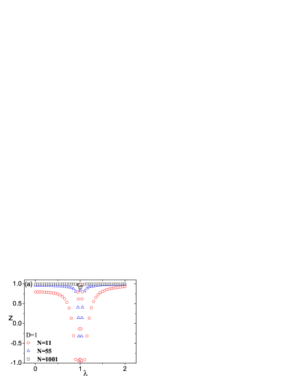
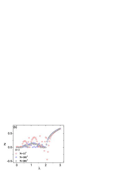
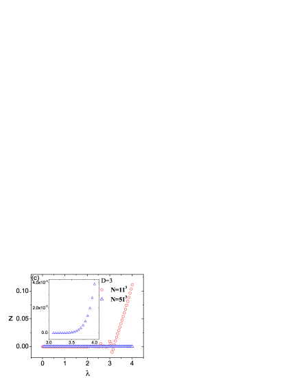
Figure 1: ( Color online ) The ground-state expectation value of twist operator $z$ for the $D$-dimensional free-fermion model vs the parameter $\lambda$. We have chosen $\gamma=1$ for this plot. The plotting in the inset of (c) shows the details of $\lambda>3$.

III.1 $D$-dimensional free-fermion model

The Hamiltonian is read as

$$H=\sum_{\langle{\mathbf{i,j}}\rangle}[c_{\mathbf{i}}^{\dagger}c_{\mathbf{j}}-\gamma(c_{\mathbf{i}}^{\dagger}c_{\mathbf{j}}^{\dagger}+h.c.)]-2\lambda\sum_{\mathbf{i}}c_{\mathbf{i}}^{\dagger}c_{\mathbf{i}},$$ (16)

in which $\langle\mathbf{i,j}\rangle$ denotes the nearest-neighbor lattice sites and $c_{\mathbf{i}}$ is the fermion operator. This Hamiltonian, first introduced in Ref.li06 , depicts the hopping and pairing between nearest-neighbor lattice sites, in which $\lambda$ is the chemical potential and $\gamma$ is the pairing potential. Eq.(16) could be considered as a $D$-dimensional generalization of one-dimensional spin-$1/2$ $XY$ model. However for the $D>1$ case, this model shows some novel phase characteristics li06 .

Eq. (16) can be resolved exactly by transforming into moment space with periodic boundary condition. Wiht the help of the Bogoliubov transformation li06 , one has

$$H=\sum_{\mathbf{k}}2\Lambda_{\mathbf{k}}\eta_{\mathbf{k}}^{\dagger}\eta_{\mathbf{k}}+const.$$ (17)

in which $\Lambda_{\mathbf{k}}=\sqrt{t_{\mathbf{k}}^{2}+\Delta_{\mathbf{k}}^{2}}$, $t_{\mathbf{k}}=\sum_{\alpha=1}^{D}\cos k_{\alpha}-\lambda$ and $\Delta_{\mathbf{k}}=\gamma\sum_{\alpha=1}^{D}\sin k_{\alpha}$. The phase diagram can be determined based on the gapless excitation $\Lambda_{k}=0$ li06 . For $D=1$, which corresponds to the one dimensional spin-$1/2$ $XY$ model, the energy gap above the ground state is non-vanishing except at $\lambda_{c}=1$ for $\gamma\neq 0$, where a second-order quantum phase transition occurs. For $\gamma=0$ the energy of the ground state is degenerate in the region $|\lambda|\leq 1$ and the transition occurs at $\lambda=\pm 1$. When $D=2$, the phases diagram should be identified with respect to two different situations; for $\gamma=0$, the degeneracy of the ground state occurs when $\lambda\in[0,2]$, whereas the gap above the ground state is non-vanishing for $\lambda>2$. However for $\gamma\neq 0$ three different phases can be identified as $\lambda=0$, $\lambda\in(0,2]$ and $\lambda>2$. The first two phases correspond to case that the energy gap for the ground state vanishes, whereas not for $\lambda>2$. One should note that $\gamma=0$ means a well-defined Fermi surface with $k_{x}=k_{y}\pm\pi$, whose symmetry is lowered by the presence of $\gamma$ terms. For $D=3$ two phases can be identified as $\lambda\in[0,3]$ with the vanishing energy gap above the ground state and $\lambda>3$ with a non-vanishing energy gap above ground state. In a word the critical points can be identified as $\lambda_{c}=D(D=1,2,3)$ for any anisotropy of $\gamma$, and $\lambda=0$ for $D=2$ with $\gamma>0$.

Defining the fermion-pair operator $\mathbf{c}_{\mathbf{i}}=(c,c^{\dagger})^{T}_{\mathbf{i}}$ and transforming the system into moment space, one then obtain

$$H=\sum_{\mathbf{k}}\mathbf{c}^{\dagger}_{\mathbf{k}}\left(\begin{array}[]{cc}\lambda-\sum_{\alpha}\cos k_{\alpha}&-i\gamma\sum_{\alpha}\sin k_{\alpha}\\ i\gamma\sum_{\alpha}\sin k_{\alpha}&-\lambda+\sum_{\alpha}\cos k_{\alpha}\end{array}\right)\mathbf{c}_{\mathbf{k}}$$ (20)

It is worth noting $\mathbf{R(k)}=(0,\gamma\sum_{\alpha}\sin k_{\alpha},\lambda-\sum_{\alpha}\cos k_{\alpha})$ and $R\mathbf{(k)}=\Lambda_{\mathbf{k}}$. $R_{y}(\mathbf{k})$ is obviously satisfied the requirement $R_{y}(\mathbf{k})=-R_{y}(-\mathbf{k})$. Substituted into Eq. (14), one obtain

$$\gamma_{g}=\text{Arg}z_{\mu}=\text{Arg}\prod_{\alpha=1}^{D}\prod_{k_{\alpha},k_{\mu}}\cos\frac{2\pi}{N}|K_{\mu}|,$$ (21)

in which $\mu=1\dots D$ and

$$K_{\mu}=-\frac{i\gamma(\lambda-\sum_{\alpha}\cos k_{\alpha})[\cos k_{\mu}(\lambda-\sum_{\alpha}\cos k_{\alpha})-\sin k_{\mu}\sum_{\alpha}\sin k_{\alpha}]}{2[\gamma^{2}(\sum_{\alpha}\sin k_{\alpha})^{2}+(\lambda-\sum_{\alpha}\cos k_{\alpha})^{2}]^{3/2}}.$$ (22)

The schematic drawing of $z$ for $D=1,2,3$ have been presented in Figs. 1, in which we have chosen $\gamma=1$ for specification. Some different characters can be found in the figures note .

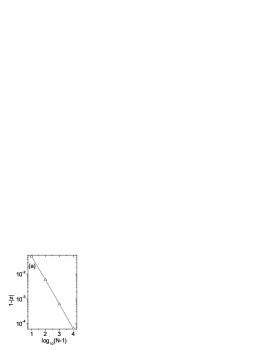
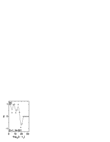
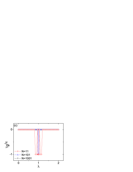
Figure 2: ( Color online )(a) $z$ for $\lambda=1$ ( plotted by a logarithm ) vs the particle number $N$ for $D=1$; (b) the asymptotic behavior of $z$ closed to transition point $\lambda=1$ for $D=1$; (c) the geometric phase $\gamma_{g}$ for $D=1$. We have chosen $\gamma=1$ for all plots.

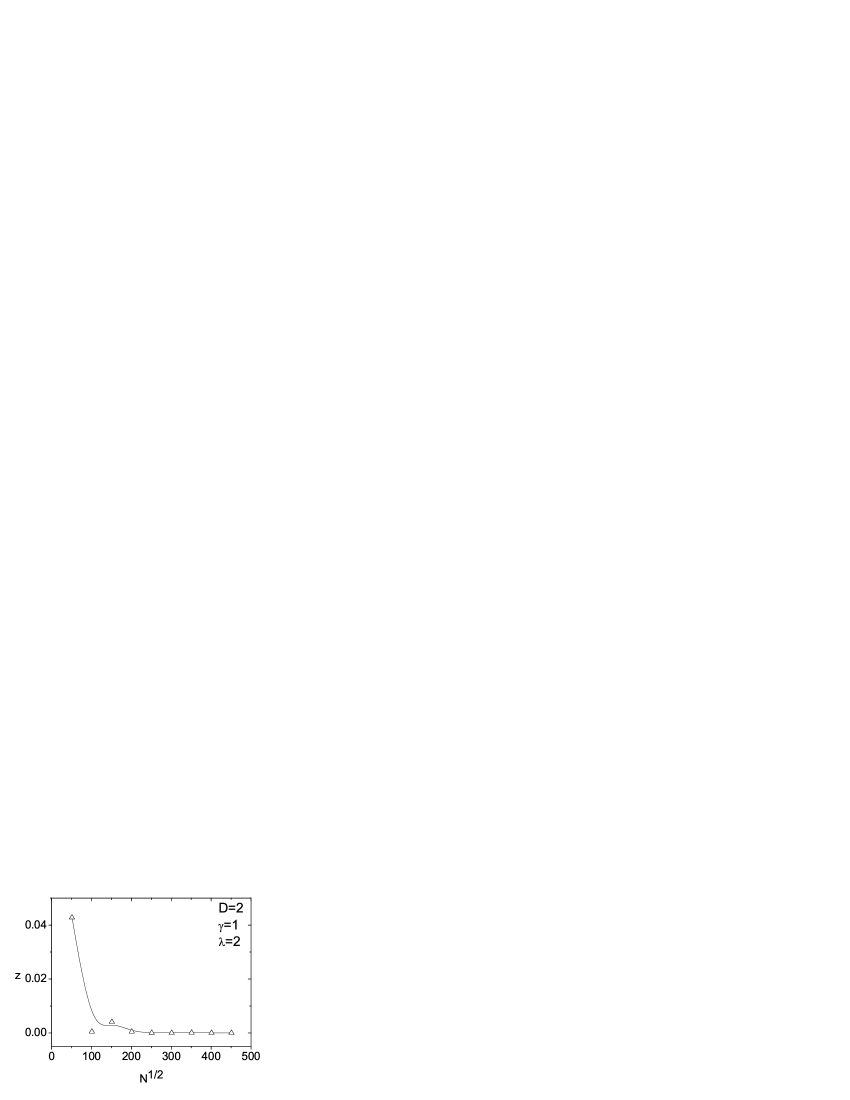
Figure 3: $z$ for $D=2$ vs particle number $N$ at phase transition point $\lambda=2$.

$D=1$. It is the well-known one-dimensional $XY$ model for this case, in which there is a quantum phase transition at $\lambda=1$ because of the degeneracy of the ground-state energy. $z$ are plotted with $\lambda$ respectively in Fig. 1 (a). It is obvious that $z$ has an dropping and then an abrupt increment when one approaches the phase transition point $\lambda_{c}=1$. Moreover our calculation shows that $z$ tends to be zero with $\lambda\rightarrow 1$ as shown in Fig. 2 (b), and at exact $\lambda_{c}=1$ $z$ tends to be 1 with the increase of the lattice site number as shown in Fig. 2 (a) note2 . $\gamma_{g}$ have also been plotted in Fig. 2 (c), in which a rapid oscillation happens closed to $\lambda_{c}=1$. These phenomena mean that $\gamma_{g}$ is ill-defined closed to $\lambda=1$ and has an abrupt change at the phase transition point. Since the energy gap vanished only at $\lambda_{c}=1$, the singularity of $\gamma_{g}$ and $z$ would be directly related to the degeneracy of the ground state energy. It also hints that one could mark the transition point by detecting the point where $z=0$.

$D=2$. With the increment of dimensionality, the situation becomes more complex. We have plotted $z$ in Fig. 1 (b). It is obvious that two different regions can be identified as $\lambda\in[0,2]$ in which $z$ is disordered, and $\lambda>2$ in which $z$ is an increasing function of $\lambda$. With respect that the disappearance of the energy gap above the ground state happens when $\lambda\in[0,2]$, $z$ presents a clear identification of the phase diagram. It is a reasonable speculation from Fig. 1 (b) that $z$ may tend to be zero under the thermodynamic limit when $\lambda\in[0,2]$. Then $\gamma_{g}$ is under thermodynamic limit

$$\gamma_{g}=\begin{cases}\text{undetermined},&\lambda\leq 2\\ 0,&\lambda>2.\end{cases}$$ (23)

Our calculation also shows that $z$ tends to be zero with the increment of $N$ at the exact transition point $\lambda_{c}=2$, as shown in Fig. 3. Similar to the case of $D=1$, it may be desirable to find the point $z=0$ as a way of detecting the phase transition.

$D=3$. This case is very similar to that of $D=2$, except the phase transition happens at $\lambda_{c}=3$. $z$ has been shown in Fig. 1 (c). However in this case $z$ seems unlikely to detect the phase transition since the data in the figure has a smoothing changes at the phase transition point for large $N$, as shown in the inset of Fig. 1 (c). Only for $N=11^{3}$, there is an abrupt changs of $z$ near to the phase transition point. One should note that $z$ tends to be zero when $\lambda\in[0,3]$, in which the energy gap above the ground state disappears.

From the discussions above, one can note the great impact of the degeneracy of the ground-state energy on the geometric phase $\gamma_{g}$ or $z$; The degeneracy of the ground-state energy leads to $z=0$ or the ill-defined $\gamma_{g}$. However, this conclusion would not be made until the next example is studied in which the energy gap above the ground state does not disappear. It is interesting to give a further discussion of the geometric phase in this nontrivial case.

Unfortunately Eq. (22) seems unsuccessful in characterizing the transitions for $\gamma=0$ (the tight-binding model) since in this case $K_{\mu}$ is completely undetermined when $\lambda-\sum_{\alpha}\cos k_{\alpha}=0$. With respect to Eqs. (16) and (8), it means that $[H,\eta]=0$ since $[\sum_{\langle{\mathbf{i,j}}\rangle}c_{\mathbf{i}}^{\dagger}c_{\mathbf{j}},\sum_{\mathbf{i}}c_{\mathbf{i}}^{\dagger}c_{\mathbf{i}}]=0$ in this special case. Hence our discussion excludes this special situation since one has trivial results. One should note that the phase of $\lambda=0$ with $\gamma>0$ in $D=2$ also cannot be identified by $z$ since the transition comes from the deformation of the Fermi surface instead of the degeneracy of the ground state.

III.2 Su-Schrieffer-Heeger (SSH) model

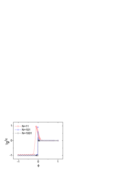
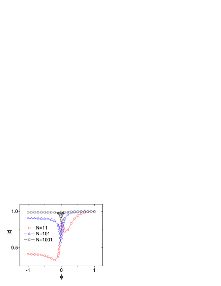
Figure 4: ( Color online ) $\gamma_{g}$ and $|z|$ for the SSH model vs. the parameter $\phi$.

Another example is the Su-Schrieffer-Heeger (SSH) model, which is also exactly solvable. The 1D tight-binding Hamiltonian for the SSH model for a chain of polyacetylene is given by heeger

$$H=\sum_{l=1}^{N}t(-1+(-1)^{l}\phi_{l})(c_{l}^{\dagger}c_{l+1}+h.c.),$$ (24)

in which $\phi_{l}$ represents the dimerization at the $l$th site and an alternating sign of the hopping elements reflects dimerization between the carbon atoms in the molecule. Without the loss of generality, it is convenient to neglect the kinetic energy in the system and take $\phi_{l}=\phi$, $t=1$ ryu2 . There is a critical point at $\phi=0$ ,which divides the ground states into two different types. One should point out that SSH has a gaped excitation for any $\phi\in[-1,1]$ and the quantum phase transition comes from the excitation of the boundary statesryu2 .

One can find from the following calculation that $\gamma_{g}$ can discriminate the two phases and the boundary between them. Defining $c_{x}=(c_{l},c_{l+1})^{T}$, the Hamiltonian becomes

$$H = \sum_{x=1}^{N}c_{x}^{\dagger}\left(\begin{array}[]{cc}0&-(1+\phi)\\ -(1+\phi)&0\end{array}\right)c_{x}$$ (27)

$$+ \left[c_{x}^{\dagger}\left(\begin{array}[]{cc}0&0\\ -1+\phi&0\end{array}\right)c_{x+1}+h.c.\right]$$ (30)

Imposing the periodic boundary condition and Fourier transformation, we then have

$$\mathscr{H}(k)=\left(\begin{array}[]{cc}0&-(1+\phi)-(1-\phi)e^{-ik}\\ -(1+\phi)-(1-\phi)e^{ik}&0\end{array}\right),$$ (31)

It is obvious that $\mathbf{R}(k)=(-(1+\phi)-(1-\phi)\cos k,-(1-\phi)\sin k,0)$ and $R_{y}(k)=-R_{y}(-k)$ is satisfied. Then

$$z=\prod_{k}(\cos\frac{2\sqrt{2}\pi}{N}|K^{\prime}|-\frac{i\text{Im}[K^{\prime}]}{\sqrt{2}|K^{\prime}|}\sin\frac{2\sqrt{2}\pi}{N}|K^{\prime}|),$$ (32)

in which $K^{\prime}=-\frac{i}{2}\frac{(1-\phi)^{2}+(1-\phi^{2})\cos k}{(1-\phi)^{2}\sin^{2}k+[1+\phi+(1-\phi)\cos k]^{2}}$.

We plot $\gamma_{g}$ against $\phi$ with different site numbers in Fig. 4. It is obvious that $\gamma_{g}$ is $-\pi$ for $\phi\in[-1,0)$ and zero for $\phi\in(0,1]$ from Fig. 4. Moreover $\gamma_{g}$ tends to be $\pi$ at exact phase transition point $\phi=0$. Furthermore our calculation shows that $|z|$ is not zero, which means that one cannot detect the phase transition by finding the point $z=0$. Since the energy gap for the ground state is nonvanishing in this model, the geometric phase $\gamma_{g}$ can be well-defined for any $\phi$. With respect to the discussion for the $D$-dimensional free-fermion system, it is evident that $\gamma_{g}$ or $z$ are directly related to the degeneracy of the ground state.

IV discussions and conclusions

Given the two examples, some comments should be presented in this section. In this paper the twist operator Eq. (1) has been introduced and its ground-state expectation $z$ has been calculated to define the geometric phase Eq. (3) for the two-band model. Although the absent of general results, the exact expression of $z$ can be obtained in a special case, which provides the ability to detect the details of the geometric phase adjacent to the phase transition points. With respect to the discussions for two representative examples-D-dimensional free-fermions model and the Su-Schrieffer-Heeger model, some distinguished properties of $\gamma_{g}$ or $z$ have been found in our calculations.

First when the degeneracy of the ground state happens, $z$ tends to be zero and the geometric phase $\gamma_{g}$ is ill-defined in this case, as shown in Figs. 1, while $\gamma_{g}$ can be well-defined when the energy of the ground state is nondegenerate, as shown in Fig. 4. This phenomenon clearly displays the intimation connection between geometric phase, defined by the ground-state expectation value of the twist operator, and the degeneracy of the ground state in many-body systems. Consequently one can find the nodal structure of the geometric phase (the situation that the geometric phase is ill-defined because of $z=0$) to detect the phase transition originated from the degeneracy of the ground state. The nodal structure of geometric phase is introduced by Fillip and Sjöqvist for the description of experimental measure of the geometric phase based on the interference, which characterizes the condition for the disappearance of the fringes and then the geometric phase is ill-defined. Second geometric phase can also present the phase diagram even if there is a energy gap above the ground state, as shown in Fig. 4, in which two different phases defined by $\gamma_{g}=-\pi$ and $0$ can be identified and the phase transition point is marked by the discontinued variation of geometric phase. In a word the geometric phase $\gamma_{g}$ displays the ability to mark the phase diagram in this discussion, whether the phase is determined by the degeneracy of the ground state or not. Hence the geometric phase can provide a more popular depiction for the phase transition.

However there still exist some problems. First is that the geometric phase seems to fail to characterize the tight-bond model ($\gamma=0$ in Eq. (16)). It is the reason that $[H,\eta]=0$, and the twist operator has a trivial effect on the ground state. Second the geometric phase fails to detect some phase transitions not originated from the degeneracy of the ground state, such as the transition from the deformation of the Fermi surface. Thirdly $\gamma_{g}$ or $z$ seems unable to detect the broken of symmetry which happens in the 1D spin-1/2 $XY$ model, as shown in Fig. 1 (a). Although there exists some defects, the geometric phase defined by the twist operator provides one another way of detecting the phase diagram for many-body systems. Moreover the flexibility of choosing $n_{x}$ in the definition of the twist operator implies that one could properly choose different physical quantities $n_{x}$ for the description of different properties of the system.

Note added. Recently we become aware of a paper which also focuses on the connection between the geometric phase and the quantum phase transition by numerical evaluation hkh . In this paper, three different phases in gapped spin chains can be defined by the geometric phase $\gamma=0,\pi,$ and undefined respectively, which is similar to our conclusions.

Acknowledgement The author(H.T.C.) acknowledges the support of NSF of China, Grant No. 10747195.

References

- (1) Subir Sachdev, Quantum Phase Transition(Cambridge University Press, Cambridge, 1999).
- (2) J. Preskill, J. Mod. Opt. 47, 127 (2000).
- (3) A. Osterloh, L. Amico, G. Falci, R. Fazio, Nature, 416, 608(2002); T. J. Osborne and M. A. Nielsen, Phys. Rev. A 66, 032110 (2002).
- (4) L. A. Wu, M. S. Sarandy, D. A. Lidar, Phys. Rev. Lett. 93, 250404 (2004).
- (5) J. I. Latorre, E. Rico and G. Vidal, Quantum Inf. Comput. 4, 48 (2004).
- (6) L. Amico, R. Fazio, A. Osterloh, V. Vedral, Rev. Mod. Phys. 80, 517 (2008) .
- (7) X. G. Wen, Phys. Rev. B 40, R7387 (1989); X.G. Wen and Q. Niu, Phys. Rev. B 41, 9377 (1990); X. G. Wen, Quantum field Theory of Many-body Systems (Oxford University Press, 2005).
- (8) Angelo C. M. Carollo and J. K. Pachos, Phys. Rev. Lett. 95, 157203 (2005); J. K. Pachos and Angelo C. M. Carollo, Phil. Trans. R. Soc. A 364, 3463 (2006).
- (9) S. L. Zhu, Phys. Rev. Lett. 96, 077206 (2006).
- (10) H. T. Cui, K, Li, X. X. Yi, Phys. Lett. A 360, 243 (2006).
- (11) M. E. Reuter, M. J. Hartmann, M.B. Plenio, Proc. Roy. Soc. Lond. A 463, 1271 (2007).
- (12) P. Zanardi, P. Giorda, M. Cozzini, Phys. Rev. Lett. 99, 100603 (2007); L. C. Venuti and P. Zanardi, ibid. 99, 095701 (2007).
- (13) N. Paunković and V. R. Vieira, Phys. Rev. E 77, 011129 (2008).
- (14) S.-L. Zhu, Int. J. Mod. Phys. B 22, 561(2008).
- (15) E. Lieb, T. Schultz, D. Mattis, Annals of Physics, 16, 407 (1961).
- (16) R. Resta, Phys. Rev. Lett. 80, 1800 (1998); R. Resta and S. Sorella, ibid. 82, 370 (1999); R. Resta, J. Phys: Condens. Matter 12, R107 (2000).
- (17) A. A. Aligia and G. Ortiz, Phys. Rev. Lett. 82, 2560 (1999); A. A. Aligia, Europhys. Lett. 45, 411 (1999).
- (18) M. Nakamura and J. Voit, Phys. Rev. B 65, 153110 (2002); M. Nakamura and S. Todo, Phys. Rev. Lett. , (2002)
- (19) S. Ryu and Y. Hatsugai, Phys. Rev. Lett. 89, 077002 (2002).
- (20) S. Ryu and Y. Hatsugai, Phys. Rev. B 73 , 245115 (2006).
- (21) It is convenient for a two-levle system to write the desity matrix as , in which the vector is real three-dimensional vector and . This vectoer is well known as the Bloch vector.
- (22) M.V. Berry, Proc. R. Soc. Lond. A 392, 45(1984).
- (23) M. Yamanaka, M. Oshikawa, I. Affleck, Phys. Rev. Lett. 79, 1110 (1997); A. A. Aligia and E. R. Gaglinao, Physica C 304, 29 (1998); Euro. Phys. Journ. B 5, 371 (1998).
- (24) W. Li, L. Ding, R. Yu, T. Roscide and S. Haas, Phys. Rev. B 74, 073103 (2006).
- (25) Since Eq. (16) is spatially isotropic, it has no difference for with and these plottings are chosen for .
- (26) The indetermination of when can be resolvable by L’Hospital rule. Our calculation shows that is 0 for this case. For , the similar calculations are applied.
- (27) A. Heeger, S. Kivelson, J. R. Schrieffer, W. P. Su, Rev. Mod. Phys. 60, 781 (1988).
- (28) S. Filipp and E. Sjöqvist, Phys. Rev. Lett. 90, 050403 (2003); Phys. Rev. A 68, 042112 (2003).
- (29) T. Hirano, H. Katsura, Y. Hatsugai, Phys. Rev. B 77, 094431 (2008)