DMT of Multi-hop Cooperative Networks - Part II: Half-Duplex Networks with Full-Duplex Performance

Abstract

We consider single-source single-sink (ss-ss) multi-hop relay networks, with slow-fading links and single-antenna half-duplex relay nodes. While two-hop cooperative relay networks have been studied in great detail in terms of the diversity-multiplexing gain tradeoff (DMT), few results are available for more general networks. In a companion paper, we characterized end points of DMT of arbitrary networks, and established some basic results which laid the foundation for the results presented here. In the present paper, we identify two families of networks that are multi-hop generalizations of the two-hop network: $K$-Parallel-Path (KPP) networks and layered networks.

KPP networks may be viewed as the union of $K$ node-disjoint parallel relaying paths. Generalizations of these networks include KPP(I) networks, which permit interference between paths and KPP(D) networks, which possess a direct link between source and sink. We characterize the DMT of these families of networks completely for $K>3$ and show that they can achieve the cut-set bound, thus proving that the DMT performance of full-duplex networks can be obtained even in the presence of the half-duplex constraint. We then consider layered networks, which are comprised of layers of relays, and prove that a linear DMT between the maximum diversity $d_{\max}$ and the maximum multiplexing gain of $1$ is achievable for single-antenna fully-connected(fc) layered networks. This is shown to be equal to the cut-set bound on DMT if the number of relaying layers is less than $4$, thus characterizing the DMT of this family of networks completely. For multiple-antenna KPP and layered networks, we provide lower bounds on DMT, that are significantly better than the best-known bounds.

All protocols in this paper are explicit and use only amplify-and-forward (AF) relaying. We also construct codes with short block-lengths based on cyclic division algebras that achieve the optimal DMT for all the proposed schemes. In addition, it is shown that codes achieving full diversity on a MIMO Rayleigh channel achieve full diversity on arbitrary fading channels as well.

Two key implications of the results in the paper are that the half-duplex constraint does not entail any rate loss for a large class of cooperative networks and that simple AF protocols are often sufficient to attain the optimal DMT.

I Introduction

In fading relay networks, cooperative diversity provides a method of efficient operation of networks. While much of work in the literature on cooperative diversity is based on two-hop networks, we focus our attention on multi-hop networks. For a review of related literature, see Section I-A in the companion paper [1]. In the companion paper, we derived results pertaining to the DMT of arbitrary full-duplex networks.

In the present paper, we deal with half-duplex networks, for which specification of explicit schedules requires some structure in the network. Therefore, we focus on specific classes of half-duplex networks in the present paper. For half-duplex networks without a direct link, even the achievability of a maximum multiplexing gain of $1$, in the case of single antenna networks, is not clear. We will show that for a large family of networks, this maximum multiplexing gain can be achieved by appropriately scheduling the links. In fact, we will show that the cut-set upper bound on DMT for many of these networks can be achieved, thus demonstrating that the half-duplex operation does not entail any loss in DMT performance as compared to full-duplex operation for these families of networks.

I-A Classification of Networks

In this section, we define the classes of networks under consideration. The well-studied two-hop network with direct link is shown in Fig. 1. We will consider two multi-hop generalizations of two-hop networks in this paper: KPP and layered networks. Unless otherwise stated, all networks considered possess a single source and a single sink and we will apply the abbreviation ss-ss to these networks.

(a) General two-hop relay network

(b) Single relay network

Figure 1: Two-hop cooperative relay networks

A cooperative wireless network can be built out of a collection of spatially distributed nodes in many ways. For instance, we can identify paths connecting source to the sink through a series of nodes in such a manner that any two adjacent nodes fall within the Rayleigh zone[3]. This process can be continued barring those nodes which are already chosen. Such a construction will result in a set of paths from the source to the sink. In the simplest model, we can further impose the constraint that these paths do not interfere each other, see Fig.1(a), thus motivating the study of a class of multi-hop network which we shall refer to as the set of K-Parallel-Path (KPP) networks.

Figure 2: Motivation for the KPP networks

Alternatively, layers of relays can be identified from a collection of nodes between the source and the sink. This will result in a layered network model.

I-A1 Network Representation by Graph

Any wireless network can be associated with a directed graph, with vertices representing nodes in the network and edges representing connectivity between nodes. If an edge is bidirectional, we will represent it by two edges one pointing in either direction. An edge in a directed graph is said to be live at a particular time instant if the node at the head of the edge is transmitting at that instant. An edge in a directed graph is said to be active at a particular time instant if the node at the head of the edge is transmitting and the tail of the edge is receiving at that instant. Since most networks considered in this paper have bidirectional links, we will represent a bidirectional link by an undirected edge. Therefore, undirected edges must be interpreted as two directed edges, with one edge pointing in either direction.

A wireless network is characterized by broadcast and interference constraints. Under the broadcast constraint, all edges connected to a transmitting node are simultaneously live and transmit the same information. Under the interference constraint, the symbol received by a receiving end is equal to the sum of the symbols transmitted on all incoming live edges. We say a protocol avoids interference if only one incoming edge is live for all receiving nodes.

In wireless networks, the relay nodes operate in either half or full-duplex mode. In case of half-duplex operation, a node cannot simultaneously listen and transmit, i.e., an incoming edge and an outgoing edge of a node cannot be simultaneously active.

I-A2 K-Parallel-Path Networks

One way of generalizing the two-hop relay network is to consider this network as a collection of $K$ parallel, relaying paths from the source to the sink, each of length greater than $1$. This immediately leads to a more general network that is comprised of $K$ parallel paths of varying lengths, linking source and sink. More formally:

Definition 1

A set of edges $(v_{1},v_{2})$, $(v_{2},v_{3})$, $\ldots$, $(v_{n-1},v_{n})$ connecting the vertices $v_{1}$ to $v_{n}$ is called a path. The length of a path is the number of edges in the path. The K-parallel path (KPP) network is defined as a ss-ss network that can be expressed as the union of $K$ node-disjoint paths, each of length greater than one, connecting the source to the sink. Each of the node-disjoint paths is called a relaying path. All edges in a KPP network are bidirectional (see Fig. 3).

Figure 3: The KPP network

The communication between the source and the sink takes place along $K$ parallel paths, labeled with the indices $P_{1}$, $P_{2}$, $\ldots$, $P_{K}$. Along path $P_{i}$, the information is transmitted from source to sink through multiple hops with the aid of $n_{i}-1$ intermediate relay nodes $\{R_{ij}\}_{j=1}^{n_{i}-1}$.

Remark 1

A network similar to the KPP network in Definition 1 is considered in [26], albeit from a symbol error probability perspective.

Definition 1 of KPP networks precludes the possibility of either having a direct link between the source and the sink, or of having links connecting nodes lying on different node-disjoint paths. We now extend the definition of KPP networks to include these possibilities.

Definition 2

If a given network is a union of a KPP network and a direct link between the source and sink, then the network is called a KPP network with direct link, denoted by KPP(D). If a given network is a union of a KPP network and links interconnecting relays in various paths, then the network is called a KPP network with interference, denoted by KPP(I). If a given network is a union of a KPP network, a direct link and links interconnecting relays in various paths, then the network is called a KPP network with interference and direct path, denoted by KPP(I, D).

Fig. 4 below provides examples of all four variants of KPP networks.

(a) A KPP network with $K=3$

(b) A KPP(I) network with $K=3$

(c) A KPP(D) network with $K=2$

(d) A KPP(I, D) network with $K=2$

Figure 4: Examples of KPP networks.

For a KPP(D), KPP(I) or KPP(I, D) network, we consider the union of the $K$ node-disjoint paths as the backbone KPP network. While there may be many choices for the K node-disjoint paths, we can choose any one such choice and call that the backbone KPP network. These K relaying paths in these networks are referred to as the K backbone paths. A start node and end node of a backbone path are the first and the last relays respectively in the path. There are precisely $K$ start nodes in a KPP network, which are connected at one end to the source. This remains the case even for KPP(I) and KPP(I, D) networks. Similarly, sink node is connected to exactly $K$ end nodes in KPP, KPP(I) and KPP(I, D) networks.

In a general KPP network, let $P_{i},i=1,2,...,K$ be the $K$ backbone paths. Let $P_{i}$ have $n_{i}$ edges. The $j$-th edge on the $i$-th path $P_{i}$ will be denoted by $e_{ij}$ and the associated fading coefficient by $g_{ij}$.

I-A3 Layered Networks

A second way of generalizing a two-hop relay network is to view the two-hop network as a network comprising of a single layer of relays. The immediate generalization is to allow for more layers of relays between source and sink, with the proviso that any link is either between nodes in adjacent layers or connects two nodes in the same layer. We label this class of multi-hop relaying networks as layered networks:

Definition 3

Consider a ss-ss single-antenna bidirectional network. A network is said to be a layered network if there exists a partition of the vertex set $V$ into subsets $V_{0},V_{1},...,V_{L},V_{L+1}$ such that

• $V_{0},V_{L+1}$ denote the singleton sets corresponding to the source and sink respectively and for all $0<i<L+1$, $|V_{i}|\geq 2$ .

• If there is an edge between a node in vertex set $V_{i}$ and a node in $V_{j}$, then $|i-j|\leq 1$. We assume $|V_{i}|>1,i=1,2,..,L$

We will refer to $V_{1},...,V_{L}$ as the relaying layers of the network. A layered network is said to be fully-connected (fc) if for any $i$, $v_{1}\in V_{i}$ and $v_{2}\in V_{i+1}$, $(v_{1},v_{2})$ is an edge in the network. For fc layered networks, we include an additional condition that the relaying layers have at least two relays in each layer, i.e., $V_{i}>1,i=1,2,...,L$.

It must be noted that a fc layered network may or may not have links within a layer. Therefore, whenever we say fc layered network, it applies to both networks that have intra-layer links and those that do not have such links. Examples of both these types of networks are shown in Fig. 5(b) and Fig. 5(c).

Remark 2

The definition of a layered network is general enough to accommodate all ss-ss networks without a direct link. This is because, any ss-ss network can be re-drawn as a layered network with a single layer comprising of all relays in the network and interconnections between relays. For this general case, we give a certain achievable DMT.

(a) A layered network with with 4 relaying layers

(b) A fully-connected layered network

(c) A fully-connected layered network with intra-layer links

Figure 5: Examples of layered networks

Every layered network will have a layer containing only the source, and a second layer containing only the sink. In Fig.5, examples of layered networks are given. Layered networks were also considered in [18], [9] and [21]. In particular, [18] considered layered networks having an equal number of relay nodes in all layers. We will refer to such layered networks as regular networks and we will formally define them below.

Remark 3

In this remark, we characterize the intersection of KPP(I) networks and layered networks. First we observe that one is not contained in the other. Consider the subgraph of a given KPP(I) network graph, consisting of all the nodes of the original network except for the source and the sink. This subgraph will have the property that the number of node-disjoint and edge-disjoint paths is equal to the number of relay nodes immediately adjacent to the source. This is a key property of KPP(I) networks, which in general, does not hold for layered networks. On the other hand, there can be cross links between the parallel paths in a KPP(I) network in such a way that the network cannot be viewed as being layered. However, these two classes of networks are not mutually exclusive and in fact, we term networks that lie in the intersection of the two classes as regular networks.

Definition 4

A $(K,L)$ Regular network is defined as a KPP(I) network that is also, simultaneously, a layered network with $L$ layers of relays (see Fig. 6).

Figure 6: A regular network with $4$ layers and $3$ paths

Remark 4

The two-hop relay network [Fig.1(a)] is a KPP(I,D) network with $K=M$, $M$ being the number of relays. In the absence of a direct link, the two-hop relay network is a KPP(I) network with $K=M$. In fact, the two-hop relay network without direct link is also a layered network with a single layer of relays, thereby making it a $(M,1)$ regular network. On the other hand, if we have a two-hop relay network with direct link but make the additional assumption of relay isolation, then it is a KPP(D) network with $K=M$.

I-B Setting and Channel Model

We use uppercase letters to denote matrices and lowercase letters to denote vectors/scalars. Vectors and scalars are differentiated between each other by the context. Irrespective of whether it is a scalar, vector or a matrix, boldface letters are used to denote random entities.

Between any two adjacent nodes $v_{x}$ and $v_{y}$ of a wireless network, we assume the following channel model.

$$\mathbb{y}\ =\mathbb{H{x}+{w}}\ ,$$ (1)

where $\mathbb{y}$ corresponds to the received signal at node $v_{y}$, $\mathbb{w}$ is the noise vector, $\mathbb{H}$ is the channel matrix and $\mathbb{x}$ is the vector transmitted by the node $v_{x}$.

I-B1 Assumptions

We follow the literature in making the assumptions listed below. Our description is in terms of the equivalent complex-baseband, discrete-time channel.

1. All channels are assumed to be quasi-static and to experience Rayleigh fading and hence all fade coefficients are i.i.d., circularly-symmetric complex Gaussian $\mathbb{C}\mathcal{N}(0,1)$ random variables.

2. The additive noise at each receiver is also modeled as possessing an i.i.d., circularly-symmetric complex Gaussian $\mathbb{C}\mathcal{N}(0,1)$ distribution.

3. Each receiver (but none of the transmitters) is assumed to have perfect channel state information of all the upstream channels in the network.

I-C Background

We refer the reader to Section II-A.$1$ of the companion paper [1] for a background on the diversity-multiplexing gain tradeoff (DMT).

I-C1 Cut-set Bound on DMT

For each of the networks described in this paper, we can get an upper bound on the DMT, based on the cut-set upper bound on mutual information [25]. This was formalized in [3] as follows:

Lemma I.1

Let $r$ be the rate of multiplexing gain at which communication between the source and the sink is taking place. Given a cut $\omega$, there is a channel matrix $\mathbb{H}_{\omega}$ connecting the input terminals of the cut to the output terminals. Let us call the DMT corresponding to this $\mathbb{H}_{\omega}$ matrix as the DMT of the cut, $d_{\omega}(r)$. Then the DMT between the source and the sink is upper bounded by

$$d({r})\leq\ \min_{\omega\in\Lambda}\ \{d_{\omega}(r)\}\ ,$$

where $\Lambda$ is the set of all cuts between the source and destination.

Remark 5

Note that the cut-set bound does not take into account half-duplex operation of the network and therefore applies equally to both full and half-duplex networks. This clearly presents a greater challenge for half-duplex protocols.

Definition 5

Given a random matrix $\mathbb{H}$ of size $m\times n$, we define the DMT of the matrix $\mathbb{H}$ as the DMT of the associated channel $\mathbb{y=Hx+w}$ where $\mathbb{y}$ is a $m$ length received column vector, $\mathbb{x}$ is a $n$ length transmitted column vector and $\mathbb{w}$ is a $\mathbb{C}\mathcal{N}(0,I)$ column vector. We denote the DMT by $d_{H}(.)$

I-C2 Amplify and Forward Protocols

An AF protocol $\wp$ is a protocol $\wp$ in which each node in the network operates in an amplify-and-forward fashion. Such protocols induce a linear channel model between source and sink of the form:

$$\mathbb{y}\ =\mathbb{H(\wp){x}+{w}}\ ,$$ (2)

where $\mathbb{y}\in\mathbb{C}^{m}$ denotes the signal received at the sink, $\mathbb{w}$ is the noise vector, $\mathbb{H(\wp)}$ is the $(m\times n)$ induced channel matrix and $\mathbb{x}\in\mathbb{C}^{n}$ is the vector transmitted by the source. We impose the following energy constraint on the transmitted vector $\mathbb{x}$

$$\text{Tr}(\Sigma_{x})\ :=\ \text{Tr}(\mathbb{E}\{\mathbb{x}\mathbb{x}^{\dagger}\}) \leq n\rho$$

where Tr denote the trace operator, and we will regard $\rho$ as representing the SNR on the network. We will assume a symmetric power constraint on the relays and the source. However it will turn out that given our high SNR perspective, the exact power constraint is not very important. We consider both half and full-duplex operation at the relay nodes.

Our attention here will be restricted to amplify-and-forward (AF) protocols since as we shall see, this class of protocols can often achieve the DMT of a network. More specifically, our protocol will require the links in the network to operate according to a schedule which determines the time slots during which a node listens as well as the time slots during which it transmits. When we say that a node listens, we will mean that the node stores the corresponding received signal in its buffer. When a node does transmit, the transmitted signal is simply a scaled version of the most recent received signal contained in its buffer, with the scaling constant chosen to meet a transmit power constraint. In particular, nodes in the network are not required to decode and then re-encode. It turns out [2], that the value of the scaling constant does not affect the DMT of the network operating under the specific AF protocol. Without loss of accuracy therefore, we will assume that this constant is equal to $1$.

It follows that, for any given network, we only need specify the schedule to completely specify the protocol. This will create a virtual MIMO channel of the form ${\bf y}\ =\ {\bf H}{\bf x}\ +\ {\bf w}$ where ${\bf H}$ is the effective transfer matrix and ${\bf w}$ is the noise vector, which is in general colored.

I-D Certain Results from the Companion Paper

In the companion paper [1], we developed basic results that will be instrumental in deriving the DMT of certain classes of networks in this paper. A few important results among them are given here for reference.

We proved that the correlated noise encountered at the sink of many multi-hop networks is white in the scale of interest. This result will be assumed throughout this paper and is formalized in the theorem below.

Theorem I.2

[1] Consider a channel of the form $\mathbb{y}=\mathbb{Hx}+\mathbb{z}$. Let $\mathbb{h_{1},h_{2},...,h_{L}}$ be $L$, possibly dependent, Rayleigh random variables. Let $\mathbb{G}_{i},i=1,2,..,M$ be $N\times N$ matrices in which each entry is a polynomial function of the random variables $\mathbb{h_{1},h_{2},...,h_{L}}$. Let $\mathbb{z}=\mathbb{z}_{0}+\sum_{i=1}^{M}\mathbb{G}_{i}\mathbb{z}_{i}$ be the noise vector. Let $\{\mathbb{z}_{i}\}$ be i.i.d. circularly symmetric, $n$-dimensional complex gaussian $\mathbb{C}\mathcal{N}(\underline{0},I)$ random vectors. The random matrix $\mathbb{H}$ in general depends on the random variables $\mathbb{h_{i}}$. Then $\mathbb{z}$ is white in the scale of interest, i.e.,

$$Pr(\log\det(I+\rho\mathbb{H}\mathbb{H}^{\dagger}\Sigma^{-1})\leq r\log\rho)$$

$$\doteq Pr(\log\det(I+\rho\mathbb{H}\mathbb{H}^{\dagger})\leq r\log\rho)$$

We also proved a result pertaining to the DMT of block lower triangular(blt) matrices as given below.

Theorem I.3

[1] Consider a random blt matrix $\mathbb{H}$ having component matrices $\mathbb{H}_{ij}$ of size $N_{i}\times N_{j}$. Let $M:=\sum_{i=1}^{N}N_{i}$ be the size of the square matrix $\mathbb{H}$.

Let $\mathbb{H}^{(0)}$ be the diagonal part of the matrix $\mathbb{H}$ and $\mathbb{H}^{(\ell)}$ denote the last sub-diagonal matrix of $\mathbb{H}$. Then,

1. $d_{H}(r)\geq d_{H^{(0)}}(r)$.

2. $d_{H}(r)\geq d_{H^{(\ell)}}(r)$.

3. In addition, if the entries of $H^{(\ell)}$ are independent of the entries in $H^{(0)}$, then $d_{H}(r)\geq d_{H^{(0)}}(r)+d_{H^{(\ell)}}(r)$

In this paper, we will frequently use two results on the DMT of parallel channel that are proved in the companion paper [1].

Lemma I.4

[1] Consider a parallel channel with $M$ links, with the $i$th link having representation ${\bf y_{i}}=\mathbb{H_{i}}{\bf x_{i}}+\mathbb{w_{i}}$, and let $d_{i}(\cdot)$ denote the corresponding DMT. Then the DMT of the overall parallel channel is given by

$$d(r)=\inf_{(r_{1},r_{2},\cdots,r_{M}):\ \sum_{i=1}^{M}r_{i}=r}\ \sum_{i=1}^{M}{d_{i}(r_{i})}.$$ (3)

Lemma I.5

[1] Consider a parallel channel with $M$ links and repeated channel matrices. More precisely, let there be $N$ distinct channel matrices $H^{(1)},H^{(2)},...,H^{(N)}$, with $H^{(i)}$ repeating in $n_{i}$ sub-channels, such that $\sum_{i=1}^{N}n_{i}=M$. Then the DMT of such a parallel channel is given by,

$$d(r)=\inf_{(r_{1},r_{2},\cdots,r_{M}):\ \sum_{i=1}^{N}\ n_{i}r_{i}=r}\ \sum_{i=1}^{N}{d_{i}(r_{i})}.$$ (4)

We also established that diversity of any flow in a multi-terminal network equals the min-cut between the source and the sink of that flow. The result is given in the below theorem.

Theorem I.6

[1] Consider a multi-terminal fading network with nodes having multiple antennas with edges connecting antennas on two different nodes having i.i.d. Rayleigh-fading coefficients. The maximum diversity achievable for any flow is equal to the min-cut between the source of the flow and the corresponding sink. Each flow can achieve its maximum diversity simultaneously.

We established an achievable DMT region for full-duplex networks, which is summarized in the following theorem.

Theorem I.7

[1] Consider a ss-ss full-duplex network with single antenna nodes. Let the min-cut of the network be $M$. Let the network satisfy either of the two conditions below:

1. The network has no directed cycles, or

2. There exist a set of $M$ edge-disjoint paths between source and sink such that none of the $M$ paths have shortcuts.

Then, a linear DMT $d(r)=M(1-r)^{+}$ between a maximum multiplexing gain of $1$ and maximum diversity $M$ is achievable.

I-E Results

In this paper, we characterize the DMT of KPP networks and its variants called KPP(D) and KPP(I) networks. We also provide an achievable DMT for layered networks. In many cases, the achievable DMT equals the cut-set bound and is thereby optimal. All the strategies are of half-duplex nature. We give explicit protocols and code constructions for all cases. Some of these results were presented in conference versions of this paper [13, 12, 14, 15] (see also [16, 17]).

The principal results of the paper are the following(see Table I).

1. For KPP, KPP(I) and KPP(D) networks, we propose an explicit protocol whose achievable DMT coincides with the cut-set bound.

2. For fc layered networks, we construct protocols that achieve a DMT that is linear between the maximum diversity and maximum multiplexing gain points. This DMT is optimal if the number of layers is strictly less than $4$.

3. For general layered networks, we give a sufficient condition for the achievability of a linear DMT between the maximum diversity and the maximum multiplexing gain in Lemma IV.3.

4. For KPP and layered networks with multiple antenna nodes, we examine certain protocols and establish achievable DMT for these protocols.

5. In Section VI, we give explicit codes with short block-lengths based on cyclic division algebras that achieve the best possible DMT for all the schemes proposed above. We also prove that full diversity codes for all networks in this paper can be obtained by using codes that give full diversity on a Rayleigh fading MIMO channel.

TABLE I: Principal Results Summary

Network	No of	No of	Direct	Upper bound on	Achievable	Is upper bound	Reference
	sources/	antennas	Link	Diversity/DMT	Diversity/DMT	achieved?
	sinks	in nodes		$d_{\text{bound}}(r)$	$d_{\text{achieved}}(r)$
KPP(K $\geq$ 3)	Single	Single	$\times$	$K(1-r)^{+}$	$K(1-r)^{+}$	$\checkmark$	Theorem II.9
KPP(D)(K $\geq$ 4)	Single	Single	$\checkmark$	$(K+1)(1-r)^{+}$	$(K+1)(1-r)^{+}$	$\checkmark$	Corollary II.11
KPP(I)(K $\geq$ 3)	Single	Single	$\times$	$K(1-r)^{+}$	$K(1-r)^{+}$	$\checkmark$	Theorem III.6
Fully	Single	Single	$\times$	Concave	$M(1-r)^{+}$	A linear DMT	Theorem IV.6
Connected				in general		between $d_{\max}$ and
Layered						$r_{max}$ is achieved.
						$\checkmark$ for $L<4$	Corollary IV.7
Any	Single	Single	$\times$	Cut-set	$M(1-r)^{+}$	A linear DMT	Lemma IV.3
network				Bound		between $d_{\max}$ and
satisfying						$r_{max}$ is achieved
Lemma IV.3
$(K,L)$ Regular	Single	Single	$\times$	$K(1-r)^{+}$	$K(1-r)^{+}$	$\checkmark$	Theorem III.2

I-F Outline

In Section II, we focus on half-duplex KPP networks and present protocols achieving optimal DMT for $K\geq 3$. We extend this result to KPP(D) networks at the end of this section. In Section III, KPP(I) networks with half-duplex relays are considered, and schemes achieving optimal DMT are presented for KPP(I) networks allowing certain types of interference. In Section IV, we consider layered networks and show that a linear DMT between maximum multiplexing gain and maximum diversity is achievable. In Section V, we consider multi-antenna layered and KPP networks and give an achievable DMT. Finally, in Section VI, we give explicit CDA based codes of low complexity for all the DMT optimal protocols.

II Half-Duplex Networks with Isolated Paths - KPP Networks

In this section, we consider KPP and KPP(D) networks with single-antenna nodes operating under the half-duplex constraint. Discussion on KPP(I) nertworks is deferred to a later section.

II-1 The Cut-Set Bound for KPP Networks

The cut-set (Lemma I.1) upper bound on DMT for the class of KPP networks is given by:

$$d(r)\ \leq\ K(1-r)^{+},$$

and our aim is to design protocols that attain this cut-set bound.

In this section we will present protocols for KPP networks, that permit the cut-set bound to be attained for all $K\geq 3$. For the case $K=2$, we present a lower bound to the DMT that can be achieved using an AF protocol.

II-A Full-Duplex KPP Networks

To start with, we will consider full-duplex KPP networks and review the results of the first part of this paper [1] as applied to KPP networks. Theorem I.7 gives a lower-bound on the DMT of certain classes of networks with full-duplex relays. The result applies to KPP and KPP(I) networks, even with multiple antenna nodes, and is given in the corollary below.

Corollary II.1

For the full-duplex KPP networks without direct link (i.e. KPP and KPP(I) networks), with potentially multiple antenna nodes, a DMT of $d_{\max}(1-r)^{+}$ is achievable.

When nodes have a single antenna, $K(1-r)^{+}$ turns out to be the optimal DMT. However, the characterization of optimal DMT becomes tricky when the relays are half-duplex. Most articles in the literature deal with half-duplex networks by first analyzing the networks from a full-duplex perspective and then translating the results by conceding rate loss by a factor of $2$. In this and the next section, we will show that half-duplex multi-hop networks (specifically KPP networks) operating under a suitable schedule can achieve the same DMT performance as full-duplex networks.

II-B Protocols Achieving the Cut-Set Bound for $K\geq 3$

As made clear in the introduction, we restrict our attention in this paper to the class of AF protocols under which node operations are restricted to scaling and forwarding. To completely specify the manner in which the network is operated, it remains only to identify a schedule of operation.

In all of the schedules considered here, node operations are periodic with a period of $N$ time slots. Thus all edge activations are periodic as well, and we will refer to $N$ as the cycle length of the protocol. We shall describe all our protocols in a simple manner, as an edge coloring scheme. Let $C=\{c_{1},c_{2},\ldots,c_{N}\}$ be the set of $N$ colors used in the scheme. Each color in $C$ signifies a distinct time slot within the $N$-slot protocol. There is a natural order between any two colors, inherited from the time-slots they represent within a cycle. All the edges in the network are assigned a subset of colors from the set $C$. The subset of colors assigned to the edge $e_{ij}$ will be denoted by $A_{ij}$. Each color in $A_{ij}$ represents the time instants during which the edge $e_{ij}$ is active.

Definition 6

A half-duplex protocol is said to be an orthogonal protocol if at any node, at a given time instant, only one of the incoming or outgoing edges is active. An orthogonal protocol for a KPP network is said to have the equi-activation property if each edge along a given backbone path in the KPP network is activated an equal number of times.

Remark 6

The definition of orthogonal protocol is similar in spirit to the definition in the networking literature [24], where a network is said to have orthogonal channels if interference is avoided at all nodes and each node is permitted to communicate with at most one other node at any given time.

All of the orthogonal protocols employed in this paper will satisfy the equi-activation property and hence, whenever in the sequel we speak of an orthogonal protocol, we will mean an orthogonal protocol that in addition, satisfies the equi-activation property.

Proposition 1

Every orthogonal protocol can be described as an edge coloring of the network satisfying the following constraints. Conversely, every edge coloring satisfying the following constraints describes an orthogonal protocol.

$$A_{i1}\cap A_{j1} = \phi,i\neq j.$$ (5)

$$A_{i{n_{i}}}\cap A_{jn_{j}} = \phi,i\neq j.$$ (6)

$$A_{ij}\cap A_{i(j+1)} = \phi,j=1,2,...,{n_{i}}-1.$$ (7)

$$|A_{ij}| = m_{i},j=1,2,...,n_{i}.$$ (8)

Figure 7: KPP network orthogonal protocol

The first constraint corresponds to the fact that for an orthogonal protocol, only one outgoing edge is active at the source. Similarly the second constraint corresponds to the fact that for an orthogonal protocol, only one incoming edge is active at the sink. The third constraint captures the half-duplex nature of the protocol. The last constraint corresponds to the equi-activation property of the orthogonal protocols considered here. A coloring which respects all the above constraints for an example KPP network is given in Fig. 7. In this example, the protocol has a cycle length of $4$ time-slots, represented by the colors $c_{1},c_{2},c_{3},$ and $c_{4}$ in order. Within a given cycle, each edge is activated during exactly one time-slot, specified by a color, $c_{i},$ $1\leq i\leq 4$.

Definition 7

The rate, R of an orthogonal protocol is defined as the ratio of the number of symbols transmitted by the source to the total number of time slots. In terms of the notation above, we have

$$R=\frac{\sum_{i=1}^{K}m_{i}}{N}.$$

Definition 8

Consider a KPP network. Let $v_{1},v_{2},v_{3},v_{4}$ be four consecutive vertices lying on one of the $K$ parallel paths leading from the source to the sink. Let $v_{1}$ and $v_{3}$ transmit, thereby causing the edges $(v_{1},v_{2})$ and $(v_{3},v_{4})$ to be active. Due to the broadcast and interference constraints, transmission from $v_{3}$ interferes with the reception at $v_{2}$. This is termed as back-flow, and is illustrated in Fig.8

Figure 8: Back-flow on a path

Back-flow can be avoided by ensuring that there are at least two inactive edges between any two active edges along a backbone path. We formalize this below:

Remark 7

An orthogonal protocol avoids back-flow if the edge coloring satisfies:

$$A_{ij}\cap A_{i(j+2)}=\phi,j=1,2,...,{n_{i}}-2.$$

From the remark above, it is evident that any three adjacent edges $e_{ij},e_{i(j+1)},$ and $e_{i(j+2)}$ will map to disjoint sets of colors when the coloring scheme corresponds to an orthogonal protocol that avoids back-flow. Moreover, repetition of the same set of colors along every third edge is permitted under the constraints of an orthogonal protocol avoiding back-flow. This suggests an easy way of arriving at an edge coloring that satisfies the constraints. To color the edges along a backbone path in the KPP network, we will first select three disjoint subsets of colors, order these and then repeat them cyclically along the edges of the path moving from source to sink. For reasons that will become apparent later, we may deviate from this rule with respect to the coloring of the last edge along any backbone path. More formally, for any given path $P_{i},i\in[K]$, let $G_{i}=(G_{i0},G_{i1},G_{i2})$ be the set of three colors repeated cyclically starting from the first node and let $F^{i}$ specify the subset assigned to the last edge $e_{i{n_{i}}}$ along path $P_{i}$. Then the corresponding edge coloring is given by

$${A_{ij}} = \left\{\begin{array}[]{ccc}G_{i(j\pmod{3})},&&\ \mbox{$j\neq n_{i}$}\\ F^{i},&&\ \mbox{$j=n_{i}$}\\ \end{array}\right.\ .$$ (11)

Henceforth, we will use $G^{i},F^{i}$ as descriptors of the orthogonal protocol. We show next how by adding a few additional constraints, we obtain a protocol that achieves the cut-set bound.

Lemma II.2

Consider a KPP network. If an orthogonal protocol satisfies the following constraints:

1. The rate of the protocol is equal to one.

2. In every cycle, the sink receives an equal number of symbols from each of the $K$ backbone paths.

3. The protocol avoids back-flow.

Then the protocol achieves the cut-set bound, i.e.,

$$d(r)=K(1-r)^{+}.$$

Proof:

Consider a situation when a KPP network starts operating under an orthogonal protocol satisfying the constraints above. Since the sink receives an equal number of symbols from each of the $K$ backbone paths, symbols from the source should be transmitted via each of the $K$ backbone paths equally often. Also, the protocol being of rate $1$, a symbol is transmitted from the source in every time-slot. For this reason, we treat the transmission from the source in blocks constituting of $K$ symbols, each denoted by a vector $\mathbb{x}=[\mathbb{x}_{1},\cdots,\mathbb{x}_{K}]^{t}$, in which a symbol $\mathbb{x}_{i}$ takes on backbone path $P_{i}$. Clearly, the delay encountered by each symbol depends on the length of the path it traverses. However, it also depends on the schedule of edge activations dictated by the protocol. For example, in a path $P_{1}$, consider two adjacent edges $e_{1j}$ and $e_{1(j+1)}$ with a common node $v$. If $e_{1j}$ and $e_{1(j+1)}$ are assigned with colors $c_{j}$ and $c_{j+2}$(Here, we assume that time-slots are in the same order as that of index of the color), then $v$ incurs a delay of $1$ time-slot due to the schedule. Thus each component $\mathbb{x}_{i}$ experiences the sum of delays along all the nodes in the path $P_{i}$.

This difference in delay experienced by each component $\mathbb{x}_{i}$ in $\mathbb{x}$ may be large enough so that the information corresponding to $\mathbb{x}_{i}$ arrives at the sink node during one cycle of the protocol, whereas the information corresponding to $\mathbb{x}_{i+1}$ may arrive at the sink node during some other cycle. Therefore, there is a need to synchronize these information symbols so that they arrive at the same cycle of the protocol. This can be done by adjusting the delays of each path at the source (by a multiple of $K$) so that all the symbols $\mathbb{x}_{1},...,\mathbb{x}_{K}$ in a block of data are received in the same cycle at the destination. However, the activation of the edges connecting to the sink need not be in the same order as that in which edges connected to the source are activated. Therefore, within a cycle, the symbols might be received in a different order. Hence, we shuffle the input appropriately within each cycle (it corresponds to multiplication by a permutation matrix, $P$), so that we get an input output relation between the input $\mathbb{x}$ and the output $\mathbb{y}$ as,

$$\mathbb{y} = \left[\begin{array}[]{cccc}\mathbb{g}_{1}&&&\\ &\mathbb{g}_{2}&&\\ &&\ddots&\\ &&&\mathbb{g}_{K}\\ \end{array}\right]\mathbb{x}+\mathbb{w},\$$ (16)

where $\mathbb{g}_{i}$ denotes the product fading coefficient of the path $P_{i}$, and $\mathbb{w}$ is the noise vector at the sink, which is white in the scale of interest.

Note that the initial delay, D, encountered in the transmission is not accounted for in the channel model given in (16). However, when the network operates continuously for long duration $T$, this delay does not affect in terms of loss in rate since the rate loss factor of $\frac{T-D}{T}$ can be made arbitrarily small when $T$ becomes large. We will always make this assumption whenever we are dealing with KPP, KPP(I), KPP(D) networks.

The DMT of the above matrix, $\mathbb{H}$ can be easily computed to be equal to

$$d(r) = K(1-r)^{+}.$$ (17)

∎

Remark 8

In later sections, whenever we refer to orthogonal protocols for KPP networks satisfying conditions in Lemma II.2, we assume that the protocol will induce a channel as given in (8), neglecting the initial delay. This is justified in the proof of the above lemma.

We will now show that the requirements of Lemma II.2 can be met in the case of KPP networks with $K\geq 4$:

Theorem II.3

For any KPP network with $K\geq 4$, there exists an explicit protocol achieving the cut-set bound on DMT.

Proof:

We now establish an orthogonal protocol satisfying the conditions in Lemma II.2 for the case when $K\geq 4$. We choose the cycle length of the protocol to be equal to the number of parallel paths $K$. By our earlier observations, it suffices to identify the coloring subsets $\left\{(G_{i0},G_{i1},G_{i2}),\ \ \{F_{i}\}\mid 1\leq i\leq K\right\}$ used by the protocol. These subsets are identified below:

$$G_{i} = [\{c_{i}\},\{c_{i+1}\},\{c_{i+2}\}],$$ (18)

$$F_{i} = \{c_{i+3}\}.$$ (19)

Verification that this coloring scheme meets all the constraints of Lemma II.2 is straightforward. It follows that this orthogonal protocol achieves the cut-set bound . ∎

The previous theorem handles the case when there are $4$ or more backbone paths in the KPP network. When $K=3$ it is not possible to identify efficient protocols that avoid back-flow. The lemma below reassures us that this does not prevent us from achieving the cut-set bound on the DMT.

Lemma II.4

Consider a KPP network operating under an orthogonal protocol, which on neglecting the effect of back-flow, induces a block-diagonal channel matrix. IThen, the DMT of the protocol taking into account the effect of back-flow, is lower bounded by the DMT when neglecting the effect of back-flow .

Proof:

The presence of back-flow creates entries in the strictly lower-triangular portion of the induced channel matrix. Since the DMT of a lower triangular matrix is lower bounded by the DMT of the corresponding diagonal matrix (by Theorem I.3), we have that the system with back-flow will yield a DMT no worse than the one without back-flow. ∎

We will now exploit Lemma II.4 to construct a protocol achieving the cut-set bound for the KPP network with $K=3$.

Theorem II.5

For any KPP network with $K=3$, there exists an explicit protocol achieving the cut-set bound on DMT.

Proof:

For every parallel path, $P_{i}$, define

$${a_{i}} = \left\{\begin{array}[]{ccc}1,&&\ \mbox{$n_{i}=1$ mod $3$}\\ 0,&&\ \mbox{$n_{i}\neq 1$ mod $3$}\\ \end{array}\right.\ .$$ (22)

Without loss of generality we assume that the paths are ordered such that for the first $l$ paths, $a_{i}=1$ followed by the paths for which $a_{i}=0$. We give a protocol for various possible values of $l$.

• Case 1: ($l=0,1,\ or\ 3$)

  In this case, we will give a protocol that avoids back-flow, uses all paths equally, and achieves rate 1. By Lemma II.2, this protocol will achieve the cut-set bound.

  We will specify the orthogonal protocol by specifying the activation sets $G_{i}=(G_{i0},G_{i1},G_{i2})$ and $F_{i}$ for all $i$. We begin by setting $F_{i}=G_{i(n_{i}-1\pmod{3})}$. The set of colors used is $C=\left\{c_{0},c_{1},c_{2}\right\}$.

  For $l=0$,

  $G_{i}=\left\{\begin{array}[]{ccc}\mbox{$(\{c_{i}\},\{c_{i+2}\},\{c_{i+1}\})$},&&\ \mbox{$n_{i}=0$ mod $3$}\\ \mbox{$(\{c_{i}\},\{c_{i+1}\},\{c_{i+2}\})$},&&\ \mbox{$n_{i}=2$ mod $3$}\\ \end{array}\right.\ .$

  For $l=1$,

  $G_{1}=(\{c_{0}\},\{c_{1}\},\{c_{2}\})],$

  $G_{2}=\left\{\begin{array}[]{ccc}\mbox{$(\{c_{1}\},\{c_{0}\},\{c_{2}\})$},&&\ \mbox{$n_{2}=0$ mod $3$}\\ \mbox{$(\{c_{1}\},\{c_{2}\},\{c_{0}\})$},&&\ \mbox{$n_{2}=2$ mod $3$}\\ \end{array}\right.\ ,$

  $G_{3}=\left\{\begin{array}[]{ccc}\mbox{$(\{c_{2}\},\{c_{0}\},\{c_{1}\})$},&&\ \mbox{$n_{3}=0$ mod $3$}\\ \mbox{$(\{c_{2}\},\{c_{1}\},\{c_{0}\})$},&&\ \mbox{$n_{3}=2$ mod $3$}\\ \end{array}\right.\ .$

  For $l=3$,

  $G_{i}=(\{c_{i}\},\{c_{i+1}\},\{c_{i+2}\}).$

• Case 2: ($l=2$)

  For $l=2$, it turns out that there is no orthogonal protocol that satisfies all the conditions of Lemma II.2. To handle this situation, we shall now come up with a protocol which satisfies conditions $1$ and $2$ of Lemma II.2, but does not satisfy condition $3$, i.e., the protocol will not avoid back-flow. Then, we utilize Lemma II.4 to establish that the DMT for this protocol is equal to the cut-set bound.

  Consider the protocol having the following descriptor:

  $G_{i}=(\{c_{i}\},\{c_{i+1}\},\{c_{i+2}\})$ and $F_{i}=G_{i(n_{i}-1\pmod{3})}$.

  After this assignment, we make the following modifications to $A_{ij}$,

  $A_{3(n_{3})}=\{c_{2}\},$

  $A_{3(n_{3}-1)}=\{c_{0}\}$, if $n_{3}=2\pmod{3}$.

  It can be checked that the protocol satisfies the first two conditions of Lemma II.2. While condition $3$ is not satisfied, because back-flow is present, by Lemma II.4, the presence of back-flow does not worsen the DMT and therefore, the protocol achieves the cut-set bound on DMT.

∎

II-C The Case of Two Parallel Paths

We now proceed to the handle the last remaining case, namely the case when $K=2$. As in the previous case, it turns out that it is impossible to have cut-set bound achieving orthogonal protocols that avoid back-flow. Furthermore, it is not even possible to construct a rate-$1$ orthogonal protocol with or without back-flow in general. We will first determine an upper bound to the rate of any orthogonal protocol for a KPP network with $K=2$. This will then be followed by the presentation of an orthogonal protocol which achieves this upper bound.

Theorem II.6

For any KPP network with $K=2$, the maximum achievable rate for any orthogonal protocol is given by

$$R_{max} \leq \left\{\begin{array}[]{ccc}1,&&\ \mbox{$n_{1}+n_{2}=0$ \ mod \ $2$}\\ \frac{2n_{2}-1}{2n_{2}},&&\ \mbox{$n_{1}+n_{2}=1$ \ mod \ $2$}\end{array}\right.,$$ (25)

where $n_{1}\leq n_{2}$.

Proof:

Any given orthogonal protocol can be represented as a coloring of the edges satisfying the conditions in Prop. 1. For this case of $K=2$, it will be found convenient to relabel the $n_{1}+n_{2}$ edges in the network so as to form a cycle $l_{1},l_{2},...,l_{n_{1}+n_{2}}$ of length $n_{1}+n_{2}$. The specific relabeling is given by

$$l_{j} = \left\{\begin{array}[]{cc}e_{1j}\ ,&\ j\leq n_{1}\\ e_{2(n_{2}+n_{1}+1-j)}\ ,&\ n_{1}<j\leq n_{1}+n_{2}\end{array}\right.\ .$$

We associate edge $l_{1},l_{2},...,l_{n_{1}+n_{2}}$ with color $D_{1},D_{2},...,D_{n_{1}+n_{2}}$ so that

$$D_{j} = \left\{\begin{array}[]{cc}A_{1j}\ ,&\ j\leq n_{1}\\ A_{2(n_{2}+n_{1}+1-j)}\ ,&\ n_{1}<j\leq n_{1}+n_{2}\end{array}\right.\ .$$

with a single constraint,

$$D_{j}\cap D_{(j+1)\ \pmod{\ }(n_{1}+n_{2})}=\phi,\ \ \forall j=1,2,...,n_{1}+n_{2},$$ (28)

that simultaneously meets the first three conditions laid out in Prop. 1.

Now suppose we have a coloring scheme with N colors. Then each color can be assigned to at most $\lfloor\frac{n_{1}+n_{2}}{2}\rfloor$ edges. This is because if more edges were assigned with the same color, then the half-duplex constraint would be violated. So by counting edge-color pairs in two different ways, we obtain the bound,

$$\sum_{i=1}^{2}\ \sum_{j=1}^{n_{i}}\ |A_{ij}| \leq \left\lfloor\frac{n_{1}+n_{2}}{2}\right\rfloor N,$$

$$\text{ie.},n_{1}m_{1}+n_{2}m_{2} \leq \left\lfloor\frac{n_{1}+n_{2}}{2}\right\rfloor N,$$ (29)

where $m_{i}=|A_{ij}|\forall j\in[n_{i}]$. The half-duplex constraint implies that,

$$2{m_{1}}\leq{N},$$ (30)

$$2{m_{2}}\leq{N}.$$ (31)

To find the maximum rate, we pose the maximization problem: maximize rate R = $(\frac{m_{1}}{N}+\frac{m_{2}}{N})$ subject to (29), (30), and (31). This can be easily solved to obtain,

$$\frac{m_{1}}{N} = 0.5,$$

$$\frac{m_{2}}{N} = \frac{1}{n_{2}}\left\lfloor\frac{n_{1}+n_{2}}{2}\right\rfloor\ -\ \frac{n_{1}}{2n_{2}}.$$

As a result, the maximum rate of the protocol is upper-bounded as

$$R_{max} \leq \left\{\begin{array}[]{cc}1,&\ n_{1}+n_{2}=0\pmod{2}\\ \frac{2n_{2}-1}{2n_{2}},&\ n_{1}+n_{2}=1\pmod{2}\end{array}\right.,$$ (34)

where $n_{1}\leq n_{2}$.

∎

Construction II.7

This construction establishes an orthogonal protocol for $K=2$ which achieves the maximum rate. By Prop. 1, it is sufficient to specify the coloring subsets $A_{ij}$ $\forall i,j$ or equivalently, to specify the subsets $D_{j}$.

Case 1: $(n_{1}+n_{2})=0\pmod{2}$

For this case we choose $2$ as the cycle length of the protocol in our construction. Accordingly let the set of colors be $C=\{c_{0},c_{1}\}$. Set

$$D_{j} = \left\{\begin{array}[]{ccc}\{c_{0}\}\ ,&\ j=1,3,...,n_{1}+n_{2}-1\\ \{c_{1}\}\ ,&\ j=2,4,...,n_{1}+n_{2}\end{array}\right.,$$

which essentially corresponds to coloring the cycle formed by the network alternately with the two colors $c_{0}$ and $c_{1}$.

Case 2: $(n_{1}+n_{2})=1\pmod{2}$

The coloring prescribed in Case $1$ does not work here, since the cycle is of odd length. Therefore, we resort to a different coloring in this case.

We have the set of colors $C=\{c_{1},c_{2},...,c_{N}\}$, where $N=2n_{2}$. We will add colors to $D_{j}$ using the following algorithm.

1. Step 1: $D_{j}\leftarrow\phi\ \forall j\in\{1,2,...,n_{1}+n_{2}\}$.

2. Step 2: Now we will add colors to each of the set $D_{j}$ using the following algorithm. In the algorithm, whenever we refer to $D_{j}$, with $j\notin\{0,1,2,\ldots,n_{1}+n_{2}\}$, we mean $D_{j}=D_{j\pmod{n_{1}+n_{2}}}$ and with $j=0$, we mean $D_{j}=D_{n_{1}+n_{2}}$.

   $\{$

   $\hskip 7.22743ptt\leftarrow 1;$

   $\hskip 7.22743pt\text{for}\ k=1\ \text{to}\ n_{2}\ \text{in steps of}\ 1:$

   $\hskip 7.22743pt\{$

   $\hskip 14.45377pt\text{for}\ i=1\ \text{to}\ n_{1}+n_{2}-1\ \text{in steps of}\ 1:$

   $\hskip 14.45377pt\{$

   $\hskip 21.68121pt\text{if}\ i\ \text{is odd},D_{i-k+1}\leftarrow D_{i-k+1}\cup\{c_{t}\};$

   $\hskip 21.68121pt\text{if}\ i\ \text{is even},D_{i-k+1}\leftarrow D_{i-k+1}\cup\{c_{t+1}\};$

   $\hskip 14.45377pt\}.$

   $\hskip 14.45377ptt\leftarrow t+2;$

   $\hskip 7.22743pt\}.$

   $\}.$

Proposition 2

The orthogonal protocol shown in Construction II.7 achieves the maximum rate given in Theorem  II.6.

Proof:

For Case 1, it is clear that the algorithm achieves rate $1$. For Case 2, the algorithm can be summarized as follows: During the $i$-th iteration, we fix our starting point as the $i$-th link in the longer path. We have two colors at the $i$-th iteration, $C_{2i+1}$ and $C_{2i+2}$, which we will associate alternately with the edges in the circular loop starting from the $(i-1)$-th edge in the longer path $P_{2}$. This coloring respects the half-duplex, broadcast and interference constraints, because all the constraints reduce to a single one, i.e., adjacent edges in the network viewed as a cycle shall have distinct colors. After the $n_{2}$ iterations are over, we have mapped $2n_{2}$ colors to the network. The shorter path gets $n_{2}$ colors on each edge, whereas the longer path gets $n_{2}-1$ colors on each edge. Hence the rate of the resultant protocol will be equal to $\frac{2n_{2}-1}{2n_{2}}$. This is illustrated with an example, $(n_{1},n_{2})=(3,4)$ in Fig. 9.

(a) Time slots 1 and 2

(b) Time slots 3 and 4

(c) Time slots 5 and 6

(d) Time slots 7 and 8

Figure 9: Protocol Illustration: ($n_{1}$, $n_{2}$) = (3,4)

∎

Theorem II.8

For a KPP network with $K=2$, if the two path lengths are equal modulo $2$, then the DMT achieved by the orthogonal protocol of Construction II.7 meets the cut-set bound, i.e., $d(r)=2(1-r)^{+}$.

Proof:

The proof follows from Lemma II.2, Theorem II.6 and Prop. 2.∎

Theorem II.9

For a KPP network, there exists an orthogonal protocol achieving the cut-set bound if $K\geq 3$ or $K=2$ and $n_{1}=n_{2}\pmod{2}$.

Proof:

Follows from Theorem II.3, Theorem II.5 and Theorem II.8. ∎

II-D KPP Networks with Direct Link

Theorem II.10

For KPP(D) networks, the cut-set bound on DMT is achievable whenever there is an orthogonal protocol for the backbone KPP network satisfying the conditions of Lemma II.2.

Corollary II.11

For KPP(D) networks, the cut-set bound on DMT is achievable whenever $K\geq 4$.

Proof:

(of Theorem II.10)

The same protocol in the backbone KPP network yields an induced channel matrix, which is a diagonal matrix with the $K$ path gains appearing cyclically along the diagonal. In the presence of a direct link, as is the case here, clearly it is the path gain $\mathbb{g}_{d}$ of the direct link that will appear along the diagonal of the induced channel matrix. The path gains of the backbone paths will appear in general below the main diagonal. However it is not hard to see that by suitably delaying symbols along each of the $K$ paths, the path gains $\mathbb{g}_{i},i=1,2,\ldots,K$ can be made to appear cyclically along a single sub-diagonal, say the $D$-th sub-diagonal.

Figure 10: KPP(D) network protocol

For instance, consider a KPP(D) network with $4$ relaying paths (see Fig. 10). The figure describes an orthogonal protocol with the aid of a coloring using a set of colors $\{c_{1},c_{2},c_{3},c_{4}\}$. The cycle length of the protocol is $4$, and $c_{i}$ represents the $i$th time-slot within a cycle. Unlike the case in KPP networks, there is no initial delay between the start of transmission at the source and the reception at the sink, due to the presence a direct link. However, the delays encountered by symbols in various backbone paths are potentially different. In this example, delay in paths $P_{1}$ and $P_{3}$ are $7$ time-slots, whereas that in paths $P_{2}$ and $P_{4}$ are $3$ time-slots. So if the fading coefficient along the path $P_{i}$ is ${\bf g}_{i}$ and that along the direct link is ${\bf g}_{d}$, then the input-output relation between the first $10$ transmitted and received symbols would be of the form:

$${\bf y} = {\bf H}{\bf x}+{\bf w},\text{ where}$$

$$H = \left[\begin{array}[]{cccccccccc}{\bf g}_{d}&&&&&&&&&\\ &{\bf g}_{d}&&&&&&&&\\ &&{\bf g}_{d}&&&&&&&\\ &&&{\bf g}_{d}&&&&&&\\ &{\bf g}_{2}&&&{\bf g}_{d}&&&&&\\ &&&&&{\bf g}_{d}&&&&\\ &&&{\bf g}_{4}&&&{\bf g}_{d}&&&\\ {\bf g}_{1}&&&&&&&{\bf g}_{d}&&\\ &&&&&{\bf g}_{2}&&&{\bf g}_{d}&\\ &&{\bf g}_{3}&&&&&&&{\bf g}_{d}\\ \end{array}\right].$$

Here ${\bf x}$, ${\bf y}$, and ${\bf w}$ represent the input, output and noise vectors respectively, each of length $10$.

By adding a delay of $4$ time-slots at $R_{2}$ and $R_{4}$, the effective delay encountered by symbols traveling via paths $P_{2}$ and $P_{4}$ can be made to equal $7$ time-slots. The cycle length of the protocol being $4$, a delay of $4$ can be introduced by idling the respective nodes for one cycle of the protocol. This will result in a new channel matrix ${\bf H}^{\prime}$ between the same input and output vectors ${\bf x}$ and ${\bf y}$, where

$${\bf H}^{\prime}=\left[\begin{array}[]{cccccccccc}{\bf g}_{d}&&&&&&&&&\\ &{\bf g}_{d}&&&&&&&&\\ &&{\bf g}_{d}&&&&&&&\\ &&&{\bf g}_{d}&&&&&&\\ &&&&{\bf g}_{d}&&&&&\\ &&&&&{\bf g}_{d}&&&&\\ &&&&&&{\bf g}_{d}&&&\\ {\bf g}_{1}&&&&&&&{\bf g}_{d}&&\\ &{\bf g}_{2}&&&&&&&{\bf g}_{d}&\\ &&{\bf g}_{3}&&&&&&&{\bf g}_{d}\\ \end{array}\right].$$

So the effective channel matrix due to an orthogonal protocol in a KPP(D) network will be of the form,

$${\bf H}=\left[\begin{array}[]{cccccccc}{\bf g}_{d}&&&&&&&\\ &{\bf g}_{d}&&&&&&\\ &&\ddots&&&&&\\ {\bf g}_{1}&&&&&&&\\ &{\bf g}_{2}&&&&&&\\ &&\ddots&&&\ddots&&\\ &&&{\bf g}_{K}&&&{\bf g}_{d}&\\ &&&&{\bf g}_{1}&&&{\bf g}_{d}\\ \end{array}\right].$$

Next, consider the situation when the network is operated for a duration of $M=mK+D$ time-slots, for some positive integer $m$. We now invoke Theorem I.3 to the induced channel matrix ${\bf H}$ to arrive at a lower bound on the DMT as,

$$d_{H}(r) \geq d_{H^{(0)}}(r)+d_{H^{(\ell)}}(r)$$

$$\geq (1-\frac{r}{M})^{+}+K(1-\frac{r}{M-D})^{+}.$$

$$\Rightarrow d(r) = d_{H}(Mr)$$

$$\geq (1-{r})^{+}+K(1-\frac{M}{M-D}r)^{+},$$

which, as $M$ tends to infinity, becomes

$$d(r)\geq(K+1)(1-r)^{+}.$$ (37)

For KPP(D) networks, the cut-set upper bound on DMT (Lemma I.1) yields $d(r)\leq(K+1)(1-r)^{+}$. Combining this with the DMT lower bound (37), we get

$d(r)=(K+1)(1-r)^{+}$. ∎

Remark 9

Since a two-hop relay network possessing $N$ relays with direct link and with relays isolated is a KPP(D) network with $K:=N$, the DMT optimal strategy for these family of networks is given by Corollary II.11. This turns out to be the same strategy as SAF protocol given in [10] for these networks.

III Half-Duplex KPP(I) Networks

In this section, we move on to consider multi-hop networks with interference. We consider KPP(I) networks with single antenna nodes operating under the half-duplex constraint. We will show that even here, the cut-set bound can be achieved using AF protocols. The cut-set bound (Lemma I.1) gives the same DMT upper-bound $d(r)\leq K(1-r)^{+}$, as in the case of KPP networks. In this section, we will demonstrate that this DMT is in fact achievable.

In the case of a KPP(I) networks, we note that any protocol for the backbone KPP network automatically induces a protocol on the KPP(I) network. Although a protocol is orthogonal with respect to the backbone KPP network, it will most likely result in a protocol on the KPP(I) network that is not orthogonal because in the presence of interfering links, interference avoidance is no longer guaranteed. The aim here is to come up with a protocol for the backbone KPP network that induces a derived protocol on the KPP(I) network such that it will result in a DMT-achieving channel matrix for the KPP(I) network. As explained in the case of KPP networks, without loss of optimality, we can neglect the initial delay here also while considering the effective channel matrix induced by the protocol between the source and the sink. We begin by introducing the notion of causal interference.

III-A Causal Interference

Definition 9

Let ${\bf H}$ denote the channel matrix induced by an AF protocol $\wp$ employed in a KPP(I) network $\mathcal{N}$. Let ${\bf H}^{(0)}$ be the diagonal part of ${\bf H}$. Let ${\bf H}_{bb}$ denote the channel matrix induced by $\wp$ when it is employed on the backbone of $\mathcal{N}$. Then $\wp$ is said to be a causal protocol (i.e., a protocol with causal interference) if the interference admitted by the protocol is causal in nature, i.e.,

1. ${\bf H}$ is lower triangular and

2. ${\bf H}_{bb}$ = ${\bf H}^{(0)}$.

Remark 10

Note that condition 2) in the definition above is satisfied only if the protocol $\wp$ is derived from a protocol that is orthogonal with respect to the backbone KPP network. For this reason, all the protocols $\wp$ for KPP(I) networks encountered in this section will be derived from orthogonal protocols for the backbone KPP network. Thus throughout the remainder of this section, whenever the word protocol appears in the context of KPP(I) networks, it should be interpreted to mean a protocol derived from an orthogonal protocol for the backbone KPP network.

Lemma III.1

Consider a KPP(I) network operating under a causal protocol $\wp$. Let the induced channel matrices on the KPP(I) and backbone KPP networks be given by ${\bf H}$ and ${\bf H}_{bb}$ respectively. Then the DMT of $d_{H}(r)\ \geq\ d_{H_{bb}}(r)$. Furthermore, if the protocol achieves the cut-set bound on the backbone KPP network, i.e., $d_{H_{bb}}(r)\ =\ K(1-r)^{+}$, then it also achieves the cut-set bound on the KPP(I) network, i.e., $d_{H}(r)=K(1-r)^{+}$.

Proof:

Since the interference caused by the protocol is causal, ${\bf H}$ is lower triangular. We also have that ${\bf H}^{(0)}={\bf H}_{bb}$ is the diagonal part of ${\bf H}$. The lemma now follows because by Theorem I.3, the DMT of a lower triangular matrix is lower bounded by the DMT of the corresponding diagonal matrix, i.e., $d_{H}(r)\ \geq\ d_{H_{bb}}(r)$. The rest follows since the same cut-set bound also applies to the KPP(I) network. ∎

We now give a sufficient condition for a protocol to be causal.

Proposition 3

Consider a KPP(I) network under a protocol $\wp$. Then $\wp$ is causal if the unique shortest delay experienced by every transmitted symbol is through a backbone path.

Proof:

The proof is straightforward. ∎

Proposition 4

Consider a KPP(I) network under a protocol $\wp$ derived from a protocol that achieves the cut-set bound on the KPP network. If the unique shortest delay experienced by every transmitted symbol is through a backbone path, then $\wp$ achieves the optimal DMT of $d(r)=K(1-r)^{+}$.

Proof:

The proof is clear by combining Prop. 3 and Lemma III.1. ∎

III-B Optimal DMT for Regular Networks

For the class of regular networks, the sufficient condition given in Prop. 4 is easily satisfied, leading to the following result.

Theorem III.2

The optimal DMT $d(r)=K(1-r)^{+}$ of (K, L) regular networks is achievable.

Proof:

Consider a (K, L) regular network. This network can be regarded as a KPP(I) network in which each backbone path has an equal number of edges. We operate the network using a protocol that is derived from an orthogonal protocol specified for the backbone KPP network. The orthogonal protocol for the backbone KPP is specified by giving the coloring sets. The cycle length of the protocol is $K$, and hence we use the set of colors $C=\{c_{0},c_{1},\ldots,c_{K-1}\}$, and assume $\forall\ell>K,c_{\ell}=c_{\ell\pmod{K}}$. The coloring set for edge $e_{ij}$ is given by,

$$A_{ij}=\{c_{i+(j-1)}\},\ \ 1\leq i\leq K,\ 1\leq j\leq L+1.$$ (38)

An example of this coloring scheme for the network in Fig. 6 is given in Fig. 11.

Figure 11: Regular network with the protocol

It can be verified that the shortest delay encountered by every symbol is through a backbone path. It can also be checked that the protocol satisfies conditions of Lemma II.2 and thus achieves the cut-set bound on the backbone KPP network. Thus the conditions of Prop. 4 are satisfied and hence proposed protocol achieves the cut-set bound on the (K, L) regular network. ∎

Corollary III.3

For the two-hop relay network without direct link, the optimal DMT is achieved irrespective of the presence or absence of links between relays.

Proof:

The two-hop relay network without the direct link is a (K,1) regular network, where $K$ denotes the number of relays in the network. This holds irrespective of the presence of links between relays, since they only contribute to intra-layer links. Thus Theorem III.2 implies this corollary. ∎

Remark 11

The result in Corollary III.3 was also proven in a parallel work [19]. The protocols used in this paper and in [19] are essentially the same as the slotted-amplify-and-forward (SAF) protocol [10], except that the protocol is applied to a network that does not have a direct link. However, the proof techniques used here and in [19] are very different.

III-C Causal Interference for KPP(I) Networks with $K=3$

In this subsection, we construct a protocol satisfying the conditions of Prop. 4 and thereby, the protocol will be optimal. The protocol will turn out to require the introduction of suitable delays at intermediate nodes in the network. We begin by considering KPP(I) networks with $K=3$. Subsequently, we will use the theory developed here for $K=3$ to handle the case $K>3$.

Lemma III.4

For any KPP(I) networks with $K=3$, there exists a causal protocol that achieves the cut-set bound when used on the back-bone KPP network.

Proof:

The proof is deferred to Appendix A. ∎

Theorem III.5

For any KPP(I) network with with $K=3$, there exists an explicit protocol that achieves the cut-set bound on the DMT.

Proof:

In Lemma III.4, we showed how to construct an orthogonal protocol that admits causal interference. This lemma along with Lemma III.1 proves the theorem. ∎

III-D Optimal DMT of KPP(I) networks

In the last section, we have shown how to design protocols for KPP(I) networks which admit causal interference. This leads to the following results on the optimal DMT of KPP(I) networks with $K\geq 3$.

Theorem III.6

Consider any KPP(I) network with $K\geq 3$. The cut-set bound on the DMT $d(r)=K(1-r)^{+}$ is achievable.

Proof:

For $K=3$, it follows from Theorem III.5.

Now, we will consider the case when $K>3$. First we use the procedure illustrated in Lemma A.1 in order to remove all non-contiguous $k$-switches for $2\leq k\leq K$. This will lead us to a modified KPP(I) network which does not contain any non-contiguous $k$-switches. Consider a $3$PP sub-network of this KPP(I) network. From Lemma III.4, it follows that we can design a causal protocol for such a network which results in an induced channel matrix with three product coefficients corresponding to the three back-bone paths along the diagonal. There are now $K\choose 3$ possible $3$PP subnetworks of the modified KPP(I) network. If each of these subnetworks is activated in succession, it would yield a lower triangular matrix with all the $K$ product coefficient $g_{i}$ repeated $K-1\choose 2$ times along the diagonal. By Theorem I.3, the DMT of this matrix is no worse than that of the diagonal matrix alone. The diagonal matrix has a DMT equal to $K(1-r)^{+}$ after rate normalization. Therefore a DMT of $d(r)\geq K(1-r)^{+}$ can be obtained. However, since $d(r)\leq K(1-r)^{+}$ by the cut-set bound, we have $d(r)=K(1-r)^{+}$. ∎

IV Half-Duplex Layered Networks

In this section, we consider half-duplex layered networks with single-antenna nodes. As in the case of KPP(I) networks, an achievable DMT for layered networks with full-duplex relays comes as an immediate consequence of Theorem I.7. It is given in the below corollary.

Corollary IV.1

For the full-duplex layered networks, a linear DMT between the maximum diversity and maximum multiplexing gain can be achieved.

Half-duplex layered networks are typically treated by first considering full-duplex operation and then activating alternate layers in order to satisfy the half-duplex constraint [9], [21]. However, this leads to a rate loss of a factor of two. We will demonstrate in this section that there exists schedules for which this rate loss is not incurred.

We will prove that the same result holds good for fully-connected (fc) layered networks even when the relays are of half-duplex nature. First, we will establish a sufficient condition for a layered network, such that a linear DMT of $d_{\max}(1-r)^{+}$ is achievable. Also, we will prove that $d_{\max}(1-r)^{+}$ is always achievable for the fc layered networks.

IV-A Linear DMT in Layered Networks

Similar to the case of KPP networks, the basic idea is to activate $d_{\max}$ paths from the source to the sink using AF protocol. In the case of KPP networks, clearly we have $d_{\max}=K$ node-disjoint paths, and we could activate them without interference between one another. In the case of layered networks, we begin with identifying node-disjoint paths from all possible paths from the source to the sink. A path from source to sink in a layered network is said to be forward-directed if all the edges in the path are directed from one layer to the next layer towards the sink (i.e., no edge in the path goes from one layer to the previous layer and there is no edge which starts and ends in the same layer). Identification of node-disjoint forward-directed paths will allow us to schedule the edges in the network in a similar fashion as how the parallel paths in KPP network were scheduled. In the following lemma, we propose a technique to identify node-disjoint paths in a layered networks.

Definition 10

Given a set of forward-directed paths $P$ in a layered network, the bipartite graph corresponding to $P$ is defined as follows:

• Construct a bipartite graph with vertices corresponding to paths in $P$ on both sides.

• Connect a vertex associated with path $P_{i}$ on the left to a vertex associated with $P_{j}$ on the right if the two paths are node disjoint.

Lemma IV.2

Consider a set of paths $P=\{P_{i},i=1,2,\ldots,N\}$ in a given layered network. Let the product of the fading coefficient on the $i$-th path $P_{i}$ be ${\bf g}_{i}$. Construct the bipartite graph corresponding to $P$. If there exists a complete matching in this bipartite graph, then these paths can be activated in such a way that the DMT of this protocol is greater than or equal to the DMT of a parallel channel with fading coefficients ${\bf g}_{i},i=1,2,...,N$ with the rate reduced by a factor of $N$, i.e., $d(r)\geq d_{H_{d}}(Nr)$, where $H_{d}\ =\ \text{diag}({\bf g}_{1},{\bf g}_{2},\ldots,{\bf g}_{N})$.

Proof:

Suppose there is a complete matching $\pi$ on the graph constructed as above. The complete matching specifies for every path on the left $P_{i}$, a partner on the right $P_{\pi_{i}}$. The length of each path and therefore the delay is equal to $D:=L+1$ since the network is layered with $L$ relaying layers. Consider operating the network under the following protocol.

Step 1: Set $i=1$. Consider the path $P_{i}$ along with its partner path $P_{\pi_{i}}$ as a two parallel path KPP(I) network with backbone paths of equal length. This sub-network is in fact a $(2,L)$ regular network with $L$ being the number of layers in the original network. The sub-network is activated using the protocol specified in the proof of Theorem III.2 for $T>>2$ cycles, and since each protocol cycle is of duration $2$ time slots, the total length of activation is $2T$ time slots. Since the protocol is causal, it will induce a lower triangular channel matrix between the input and the output with channel gains ${\bf g}_{i}$ and ${\bf g}_{\pi_{i}}$ alternating along the diagonal.

Step 2: Repeat Step 1 for $i=2,3,\ldots,N$.

The induced channel matrix ${\bf H}$ will be a lower triangular $2NT\times 2NT$ matrix with each of ${\bf g}_{1},{\bf g}_{2},\ldots,{\bf g}_{N}$ appearing for $2T$ time-slots.

Now the DMT of the protocol $d(r)$ can be related to the DMT of the diagonal part ${\bf H}^{(0)}$ as $d(r)=d_{H}(2NTr)\geq d_{H^{(0)}}(2NTr)$ by applying Theorem I.3. If ${\bf H}_{d}$ is a $N\times N$ diagonal matrix comprising of ${\bf g}_{1},{\bf g}_{2},\ldots,{\bf g}_{N}$ along the diagonal, then $d_{H^{(0)}}(r)=d_{H_{d}}(\frac{r}{2T})$ by applying Lemma I.5. This yields $d(r)\geq d_{H_{d}}(Nr)$. ∎

We utilize the above lower bound to obtain a sufficient condition that guarantees that a linear DMT between the maximum diversity and multiplexing gain is achieved on a general layered network in the following lemma.

Lemma IV.3

For a general layered network, a DMT of $d(r)\geq M(1-r)^{+}$ is achievable whenever the network has $M$ forward-directed edge-disjoint paths from the source to the sink and the bipartite graph corresponding to the set of edge-disjoint paths $e_{i}$, $i=1,2,...,M$ has a complete matching.

Remark 12

Since an arbitrary network without a direct link can be represented as a general layered network by Remark 2, this lemma applies to arbitrary networks. If in addition to the requirements in the lemma above, the network has the number of forward-directed edge-disjoint paths equal to the min-cut, then a linear DMT of $d_{\max}(1-r)^{+}$ is achievable.

Proof:

(of Lemma IV.3) By using Lemma IV.2 we will be able to get a DMT of $d(r)\geq d_{H_{d}}(Mr)$. But since the paths are edge-disjoint, the fading coefficients are independent, and we get $d_{H_{d}}(r)=(M-r)^{+}$ by applying Lemma I.5. Therefore, we get, $d(r)\geq M(1-r)^{+}$. ∎

Since the min-cut $M$ is equal to the maximum diversity of the network by Theorem I.6, a DMT of $M(1-r)^{+}$ signifies a DMT that is linear between the maximum diversity and the maximum multiplexing gain $1$.

IV-B Fully-Connected Layered Networks

While we have established a sufficient condition for achieving a linear DMT between maximum diversity and multiplexing gain for an arbitrary layered network, even for many fc layered networks, this sufficient condition is not satisfied. For example, a fc layered network with $(3,2,3)$ nodes does not satisfy the sufficient condition in Lemma IV.3. However, as we shall see in the sequel, this can be remedied and a linear DMT is obtainable for arbitrary fc layered networks with number of nodes in any relaying layer being at least $2$. A supporting lemma is needed before we proceed to prove this main result.

Consider an fc layered network with $L$ relaying layers. Let $\mathbb{h}^{(i)}_{j}$ be the $i$-th fading coefficient in the $j$-th hop. Let there be $R_{i}$ relay nodes in the $i$-th layer. Then the number of forward-directed paths $N$ is equal to

$$N = \prod_{i=1}^{L}R_{i}.$$ (39)

Lemma IV.4

Consider an fc layered network with $L$ relaying layers. Let there be $R_{i}$ relay nodes in the $i$-th layer. Let $P=\{P_{1},..,P_{N}\}$ be the set of all forward directed paths in the network. Then the bipartite graph corresponding to $P$ has a complete matching.

Proof:

We will prove this by producing an explicit complete matching on the bipartite graph. Let the layered network have $L$ layers. Let us fix an (arbitrary) ordering on the relays in each hop. Let the relays in the $j$-th hop be indexed $0,1,...,R_{j}-1$.

There is a one-to-one correspondence between the set of all forward-directed paths and the $L$ tuples $(b_{1},...,b_{L})$, where $b_{j}$ denotes the index of the relay in the $j$-th layer visited by that path. For any given path $P$ associated to the $L$ tuple $(b_{1},...,b_{L})$, consider a path $P^{\prime}$ associated to the tuple $(c_{1},...,c_{L})$ where $c_{i}=b_{i}+1\pmod{R_{i}}$. Clearly these two paths are node-disjoint, because $R_{i}\geq 2,\ \forall i$ by definition of fc layered network. The collection of all such pairings constitutes a complete matching on the set of all forward-directed paths. ∎

Consider an fc layered network with $N$ forward-directed paths and $L$ relaying layers. Let ${\bf g}_{i}$ denote the product fading coefficient corresponding to the forward-directed path $P_{i}$ for $i=1,2,\ldots,N$. Now, $\{{\bf g}_{i}\}$ are mutually correlated because each ${\bf g}_{i}$ is the product of Rayleigh fading coefficients of links in that path, and a link may belong to multiple paths. Next we compute the DMT of a parallel channel with $N$ sub-channels in which $i$th sub-channel corresponds to the $i$th forward-directed path in the fc layered network. Clearly, the coefficient of the $i$th sub-channel is ${\bf g}_{i}$, which is the product of $L+1$ Rayleigh coefficients, one each chosen from $L+1$ different sets of Rayleigh coefficients. Here each of the $L+1$ sets corresponds to the set of fading coefficients of all links connecting two adjacent layers of relays.

Figure 12: Three hop layered network

For instance, consider an fc layered network with two layers of relays. (see Fig. 12) There are four forward-directed paths between the source and the sink. The product coefficients corresponding to these four paths are

$${\bf g}_{1} = {\bf h}^{(1)}_{1}{\bf h}^{(2)}_{1}{\bf h}^{(3)}_{1}$$ (40)

$${\bf g}_{2} = {\bf h}^{(1)}_{1}{\bf h}^{(2)}_{2}{\bf h}^{(3)}_{2}$$ (41)

$${\bf g}_{3} = {\bf h}^{(1)}_{2}{\bf h}^{(2)}_{3}{\bf h}^{(3)}_{1}$$ (42)

$${\bf g}_{4} = {\bf h}^{(1)}_{2}{\bf h}^{(2)}_{4}{\bf h}^{(3)}_{2}.$$ (43)

Our interest is to compute the DMT of the parallel channel with $4$ sub-channels with coefficients ${\bf g}_{1},\ldots,{\bf g}_{4}$. The DMT can not be computed using Lemma I.4 since the individual links are not independent. Intuitively, the diversity of this channel is at most two, since if ${\bf h}^{(1)}_{1}$ and ${\bf h}^{(1)}_{2}$ are both in deep fade, then the overall channel is likely in deep fade. We present the lemma below, which computes the DMT of general parallel channels with product coefficients having a certain structure. As a result of this lemma, it will follow that the example channel has a diversity of two.

Definition 11

A subset $S$ of a product set $\mathcal{H}\subset\{H^{(1)}\times H^{(2)}\times\cdots\times H^{(L+1)}\}$ is said to be $(\nu_{1},\nu_{2},...,\nu_{L+1})$-balanced if every element in $H^{(i)}$ appears precisely $\nu_{i}$ times as the $i$th coordinate of an element in $S$. Clearly we have $|S|=\nu_{i}|H^{(i)}|$.

Lemma IV.5

Let $H^{(i)}=\{{\bf h}^{(i)}_{1},{\bf h}^{(i)}_{2},\ldots,{\bf h}^{(i)}_{M_{i}}\},i=1,2,...,L+1$ be sets of i.i.d. Rayleigh fading coefficients. Now let $\mathcal{H}\subset\{H^{(1)}\times H^{(2)}\times\cdots H^{(L+1)}\}$ be a $(N_{1},N_{2},...,N_{L+1})$-balanced set and let $N=|\mathcal{H}|$. Let $N_{\max}=\max_{i=1,2,\ldots,N}N_{i}$ and $M_{\min}=\min_{i=1,2,\ldots,L+1}M_{i}$. Let $\psi:\mathcal{H}\rightarrow G$ be the product map such that $\psi((a_{1},a_{2},...,a_{L+1}))=\prod_{j=1}^{L+1}{a}_{i}$. Now let $\psi(\mathcal{H})=\{{\bf g}_{1},{\bf g}_{2},\ldots,{\bf g}_{N}\}$, where ${\bf g}_{i}=\prod_{k=1}^{L+1}{\bf h}^{(k)}_{e(i,k)}$, with $e(i,k)$ being a map from $[N]\rightarrow[M_{k}]$ for a fixed $k\in[L+1]$.

Let ${\bf H}$ be a $N\times N$ diagonal matrix with the diagonal elements given by ${\bf g}_{i}$. The DMT of the parallel channel ${\bf H}$ is a linear DMT between a diversity of $\frac{N}{N_{\max}}$ and a multiplexing gain of $N$,

$$d(r)=\frac{(N-r)^{+}}{N_{\max}}.$$ (44)

Proof:

The proof is deferred to Appendix B. ∎

Having thus established the DMT of a parallel channel with product fading coefficients, we now proceed to utilize this lemma to compute a lower bound on the DMT of fc layered networks.

Theorem IV.6

For a fully-connected layered network, a linear DMT between the maximum diversity and maximum multiplexing gain of $1$ is achievable.

Proof:

Consider an fc layered network with $L$ layers. Let there be $R_{i}$ antennas in the $i$-th layer for $i=0,1,...,L+1$. We consider the source as layer $0$, and sink as the $L+1$th layer so that $R_{0}=R_{L+1}=1$. Let $M_{i}:=R_{i-1}R_{i},i=1,2,...,L+1$ be the number of fading coefficients between the $(i-1)$-th and $i$th layer of relays.

Let $H^{(i)}:=\{{\bf h}^{(i)}_{j},j=1,2,..,M_{i}\}$ be fading coefficients of links connecting nodes in the $(i-1)$th layer to those in the $i$th layer, $i=1,2,...,L+1$. Let $N$ be the total number of forward-directed paths from source to sink, and $P_{i},i\in[N]$ be the various forward-directed paths. Let $P$ denote the set of all these forward-directed paths. Then $|P|=N=\prod_{i=1}^{L}R_{i}$. Let ${\bf g}_{i}$ be the product fading coefficient on path $P_{i}$. Let $M_{\min}=\min_{i=1}^{L+1}M_{i}$ and $N_{\max}=\max_{i=1}^{L+1}N_{i}$. Note that $M_{\min}$ corresponds to the value of the min-cut.

By Lemma IV.4, the bipartite graph corresponding to $P$ has a complete matching. The set of paths $P$ satisfies the criterion of Lemma IV.2 and therefore, we can obtain a DMT of

$$d(r) \geq d_{H_{d}}(Nr)$$ (45)

where ${\bf H}_{d}$ is an $N\times N$ diagonal matrix whose $i$th diagonal entry is ${\bf g}_{i}$. Now, we need to compute $d_{H_{d}}(r)$. We associate with every path $P_{i}$ an $L+1$ tuple of fading coefficients $\Theta_{i}=(\theta_{i1},\theta_{i2},\ldots,\theta_{i(L+1)})$, where $\theta_{ik}\in H^{(k)}$ is the fading coefficient of the $k$th link in path $P_{i}$. Now ${\bf g}_{i}$ is related to $\Theta_{i}$ as ${\bf g}_{i}=\prod_{k=1}^{L+1}\theta_{ik}$. Note that the collection of fading coefficient tuples $\Theta_{i}$ corresponding to all the paths $P_{i}\in P$ is a $(N_{1},N_{2},\ldots,N_{L+1})$-balanced subset of the cartesian product set $\{H^{(1)}\times H^{(2)}\times\cdots\times H^{(L+1)}\}$, where

$$N_{\ell} = \frac{\prod_{j=0}^{L+1}R_{j}}{R_{\ell-1}R_{\ell}}$$ (46)

represents the number of tuples $\Theta_{i}$ in which $h^{i}_{j}$ appears as a component for any $j\in[M_{\ell}]$.

We can now see that the parallel channel matrix ${\bf H}_{d}$ satisfies the conditions of Lemma I.4, which can be applied to obtain the DMT of ${\bf H}_{d}$ as

$$d_{H_{d}}(r) = \frac{(N-r)^{+}}{N_{\max}}.$$ (47)

Substituting this back in (45), we obtain a lower bound to the DMT of the protocol as

$$d(r) \geq d_{H_{d}}(Nr)$$ (48)

$$= N\frac{(1-r)^{+}}{N_{\max}}$$ (49)

$$\Rightarrow d(r) \geq M_{\min}(1-r)^{+}.$$ (50)

By Theorem I.6, we have that the maximum diversity is equal to the min-cut $d_{\max}=M_{\min}$ in any network. Therefore a DMT of

$$d(r) \geq d_{\max}(1-r)^{+}$$ (51)

is achievable. ∎

Therefore for the two-layer fc layered network example considered in Fig. 12, a DMT of $2(1-r)^{+}$ is achievable using the strategy proposed in the theorem. However this DMT is also the upper bound using the cut-set bound. Therefore the DMT for this example network is identically equal to $2(1-r)^{+}$. This is not particular to this example. For fc layered networks with $L<4$, the min-cut is either at the source side or at the sink side, and hence we have the following corollary:

Corollary IV.7

For an fc layered network with $L<4$, the cut-set bound on DMT is achievable.

Proof:

Let $n_{i}$ be the number of relays in layer $i$. Consider a layered network with $L=1$, i.e., there is only one layer. The DMT upper bound is $n_{1}(1-r)^{+}$ from the cut-set bound, which is achieved using the proposed strategy. For $L=2$, the cut-set bound on DMT is $\min\{n_{1},n_{2}\}\ (1-r)^{+}$, which is achieved. For $L=3$, it can be seen that $d_{\max}=\min\{n_{1},n_{2}\}$ and that the DMT upper bound is $\min\{n_{1},n_{2}\}\ (1-r)^{+}$, which is indeed achieved. ∎

V Networks with Multiple Antenna Nodes

In the previous sections, we considered networks with all nodes having single antennas. In this section, we consider the general case of networks with multiple antenna nodes. Specifically, we consider KPP, KPP(I) and fc layered networks under both full-duplex and half-duplex constraints. As it is difficult to characterize the DMT completely, we present lower bounds, i.e., an achievable DMT region.

V-A Full-Duplex, Fully-Connected Layered Networks

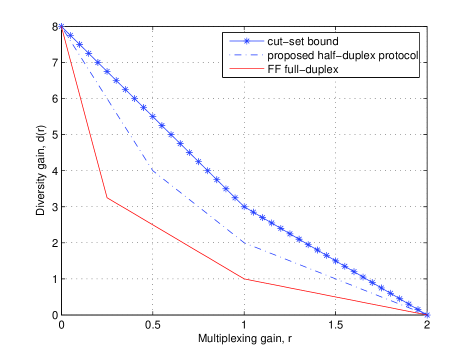
Figure 13: Comparison of various protocols for $(2,4,2)$ network

We consider fc layered networks with multiple antennas at the source and the sink. In the case of networks with multiple antennas at relays, we will replace every multiple-antena relay with an equivalent number of single-antenna relays in the same layer, and proceed to analyze the resultant network. Clearly, any protocol on the resultant network has a derived protocol in the original network and clearly the DMT of the resultant network serves as a lower bound to the DMT of the original network.

Definition 12

A ss-ss layered network with multiple antennas at the source and the sink is referred to as an $(n_{0},n_{1},\ldots,n_{L},n_{L+1})$ network if the network has $L$ layers, with the source having $n_{0}$ antennas, the sink having $n_{L+1}$ antennas, and the $i$-th layer of relays having $n_{i}$ single-antenna nodes.

In [9], parallel AF and flip-and-forward (FF) protocols have been proposed for the $(n_{0},n_{1},\ldots,n_{L+1})$ network with full-duplex operation and directed antennas. The parallel AF protocol aims to achieve the full diversity for the network, whereas FF achieves the extreme points of maximum multiplexing gain and the maximum diversity gain. In [9], it has been shown that the FF protocol achieves a better DMT than does an AF protocol. However, the DMT curves of both these protocols lie some distance away from the cut-set DMT bound. In both parallel AF and FF protocols, the key idea is to partition the relay nodes in each layer into subsets of nodes called super nodes. We propose a protocol with achievable DMT (i.e, with a lower bound to DMT) that is better than that of existing protocols for a full-duplex, $(n_{0},n_{1},\ldots,n_{L+1})$ network.

A “partitioning” $\mathfrak{p}$ of a layered network corresponds to dividing the nodes in every layer into super-nodes. We refer to the number of nodes within a super-node as the size of the super-node. Partitioning could potentially include partitioning of the source by which we mean dividing the transmit antennas of the source into super-nodes. It is similarly possible to partition the sink. Connecting any two super-nodes of size $a$ and $b$ respectively, are $ab$ edges, which we will regard as a single super-edge. We will term the resultant network comprised of super-nodes connected through super-edges as the super-network. The super-network inherits from the original network the property of being fully-connected. For a given partitioning $\mathfrak{p}$, let $S^{(\mathfrak{p})}_{i}$ be the number of super-nodes in layer $i$. The number of super-edge-disjoint paths in the super-network is equal to the min-cut of the super-network given by,

$$N^{(\mathfrak{p})} := \min_{\{i=0,1,2,...,L\}}S^{(\mathfrak{p})}_{i}S^{(\mathfrak{p})}_{i+1}.$$

We propose a protocol which uses different partitionings depending upon the multiplexing gain $r$ (we will refer to $r$ as the rate by abuse of notation). The basic intuition is that, at lower rates, we can exploit the diversity of the network by using a partitioning that results in the creation of a large number of super-edge-disjoint paths. At higher rates, we utilize a partitioning which supports enough degrees of freedom (which is equal to the minimum of the number of antennas in any super-node of an edge-disjoint path).

Let $\mathfrak{P}$ denote all possible partitionings. There can be two different partitionings in which every layer has the same number of super-nodes with corresponding sizes. However, we need to choose only one of them, as the performance of the protocol depends only on the size of super-nodes. Fix a partitioning $\mathfrak{p}$ $\in$ $\mathfrak{P}$ on the layered network. We operate the network using the following protocol: Activate all the $N^{(\mathfrak{p})}$ super-edge-disjoint paths successively so that each path is activated for $T$ time instants. During the activation of $i$th path, we will get an induced channel matrix ${\bf H}$ that is block lower-triangular with ${\bf H}^{(\mathfrak{p})}_{i}$, the product matrix for the $i$-th path appearing as the $i$th entry along the diagonal of ${\bf H}$. The induced matrix has entries in the lower triangular part of the matrix due to the presence of back-flow.

Since ${\bf H}$ is blt, by Theorem I.3, we can lower bound the DMT of this matrix by the DMT of ${\bf H}^{(0)}$, the block diagonal matrix extracted from ${\bf H}$. Let $d_{i}^{(\mathfrak{p})}(r)$ be the DMT of ${\bf H}^{(\mathfrak{p})}_{i}$, which can be computed using the techniques for computing the DMT of product Rayleigh matrices given in [9]. Now the DMT $d_{H^{(0)}}(r)$ can be computed using the parallel channel DMT in Lemma I.4 to yield the DMT of the protocol as,

$$d(r) \geq \max_{\{\mathfrak{p}\in\mathfrak{P}\}}\ \inf_{\left\{\begin{array}[]{c}(r_{1},r_{2},\cdots,r_{N^{(\mathfrak{p})}}):\\ \sum_{i=1}^{N^{(\mathfrak{p})}}r_{i}=N^{(\mathfrak{p})}r\end{array}\right\}}\ \sum_{i=1}^{N^{(\mathfrak{p})}}{{d_{i}^{(\mathfrak{p})}}(r_{i})}.$$ (54)

Since the optimization is over the set of all possible partitions, it might be difficult to compute the DMT in general. So we consider a restricted case when the source and sink are not partitioned, and all the relay layers are partitioned into the same number of super-nodes, $S$. Under this assumption, we have that $1\leq S\leq n_{\min}$, where $n_{\min}=\min\{n_{i}\}$ is the minimum number of antennas in any layer. Each super-node in the $i$th layer contains $n^{S}_{i}$ relays, where $n^{S}_{i}:=\left\lfloor\frac{n_{i}}{S}\right\rfloor,i=1,2,...,L$. The remaining $n_{i}\pmod{S}$ relays in layer $i$ are requested to be silent. This is done for simplicity of computing the DMT. Let $d_{(n_{0},n_{1},...,n_{L+1})}(r)$ denote the DMT of a product of independent Rayleigh matrices of size $n_{0}\times n_{1},n_{1}\times n_{2},...,n_{L}\times n_{L+1}$, which can be computed using the techniques given in [9]. The DMT lower bound in (LABEL:eq:MA_FD_Layered_mid) now simplifies to

$$d(r)\geq\max_{S\in\{1,2,...,n_{\min}\}}\ \ S\ d_{(n_{0},n^{(S)}_{1},...,n^{(S)}_{L},n_{L+1})}(r).$$ (56)

The strategy of Corollary IV.1 can be used to obtain a DMT of $d_{\max}(1-r)^{+}$ for any full-duplex layered network even in the presence of multiple antennas at source and sink. By combining this strategy with the aforementioned strategy and choosing the one with the better DMT based on $r$, we get a DMT of

$$d(r)\ \geq\ \max\{d_{\max}(1-r)^{+},$$

$$\max_{S\in\{1,2,...,n_{\min}\}}\ \ S\ d_{(n_{0},n^{(S)}_{1},...,n^{(S)}_{L},n_{L+1})}(r)\}.$$ (57)

The proposed protocol is essentially the same as [9] except for the following differences:

• The presentation here is not restricted to directed graphs since we are able to handle back-flow that might arise in an undirected graph by using Theorem I.3 to show that back-flow does not impair the DMT.

• The presentation here is not restricted to partitions of fixed size since evaluation of the DMT in the case of arbitrary size partitions is made possible by the use of Lemma I.4, which computes the DMT of the parallel-channel.

• Also, since we permit the size of the partition to vary with the rate, the additional flexibility can be used to improve upon the DMT attained by the FF protocol. While the dependence of network operation upon the rate could increase implementation complexity, one could adopt an intermediate strategy in which there are a small number of modes of operation, for example, two modes reserved respectively for low and high-rates.

• Finally, as will be shown in the sequel, the above results can be extended to half-duplex networks when all the relay layers are partitioned into the same number of super-nodes.

Example 1 : Consider a $(2,4,2)$ multi-antenna layered network. The achievable DMT curve using the FF protocol, the proposed protocol and the cut-set bound are plotted in the Figure 13. For rates $r\leq 0.5$, the strategy for full-duplex layered network given in Corollary IV.1 without any node-partitioning performs the best. For rates $r\geq 0.5$, partitioning the middle layer into two super-nodes with each containing two nodes performs better. A combination of these two strategies gives a superior DMT performance to the existing FF protocol.

V-B Half-Duplex Fully-Connected Layered Networks

We consider multi-antenna layered networks with the additional constraint of half-duplex relay nodes. We prove that the methods provided above for full-duplex networks can be generalized for the half-duplex network with bidirectional links.

Consider the partitioning method stated for full-duplex layered networks, with $S_{i}=S,\forall i=1,2,...,L$, i.e., the relaying layers are partitioned into equal number of super-nodes. Let the source and sink be un-partitioned. When the relay layer $i$ is partitioned into $S_{i}$ partitions, each super-node contains $n^{S}_{i}:=\left\lfloor{\frac{n_{i}}{S_{i}}}\right\rfloor$ relays. If it contains more, the remaining relays are requested to be silent, as in the full-duplex case.

The following observations are in place: Once we replace the nodes corresponding to the same partition by a super-node, this virtual network forms a regular network. This is because each relaying layer has the same number of partitions and therefore the same number of super-nodes. The resultant network being regular, we use the protocol that is given in Theorem III.2. Since the paths are of equal length, the interference is causal, making the induced channel matrix lower triangular. This has better DMT than the corresponding diagonal matrix by Theorem I.3. This yields the same lower bound on DMT as in the full-duplex case. Thus the DMT of the protocol with any given partitioning in the half-duplex case is no worse than that with full-duplex protocol under the same partitioning. So we get,

$$d(r) \geq \max\{d_{\max}(1-r)^{+},$$ (58)

$$\sup_{S\in\{2,3,..,n_{\min}\}}\ \ S\ d_{(n_{0},n^{S}_{1},...,n^{S}_{L},n_{L+1})}(r)\}.$$

The justification for retaining the term $d_{\max}(1-r)^{+}$ as part of the maximization is because the original network is fully-connected and by adopting the matching-forward-directed-paths strategy even in the presence of multiple antennas at the source and sink (see Theorem IV.6) we can achieve the same lower bound for half-duplex networks as well.

Example 2: For the case of $(2,4,2)$ network with half-duplex constraint, the proposed protocol achieves the same DMT as the full-duplex case of Example 1. However, the FF protocol used naively for a half-duplex system by activating alternative layers during alternate time slots will entail multiplexing-gain loss by a factor of $\frac{1}{2}$.

V-C KPP(I) Networks

We consider KPP(I) networks with all nodes, including the source and the sink, having multiple antennas.

V-C1 Full-Duplex KPP(I) Networks

We consider full-duplex KPP(I) networks with multiple-antenna nodes. In the case of single-antenna KPP(I) networks, we activated all backbone paths for equal durations of time in order to obtain a linear DMT in Corollary II.1. We will use a similar protocol here except that we activate different paths for different durations of time.

Let ${\bf H}_{ij}$ be the fading matrix on edge $e_{ij}$. Let the product fading matrix along backbone path $P_{i}$ be ${\bf G}_{i}$. Then ${\bf G}_{i}=\prod_{j=1}^{n_{i}}{\bf H}_{ij}$. Let the DMT corresponding to this product matrix ${\bf G}_{i}$ be $d_{i}(r)$, which can be computed according to formulae given in [9].

Since activating different paths can potentially have different DMTs, it is not optimal in general to use all paths equally. When one is operating at a higher multiplexing gain, one might want to use a path with higher multiplexing gain more frequently in order to get greater average rate. While operating at a low rate, all the paths must be used in order to get maximum diversity. We consider a generic case where path $i$ is activated for a fraction $f_{i}$ of the duration. These fractions can be chosen depending on $r$ in order to maximize $d(r)$.

By so doing, we will get a parallel channel with repeated coefficients. The DMT of such a channel was evaluated in Lemma I.5. After making suitable rate adjustments, we obtain a lower bound on the DMT of the protocol as,

$$d(r) \geq \sup_{(f_{1},f_{2},\cdots,f_{K})}\ \ \inf_{\left\{\begin{array}[]{c}(r_{1},r_{2},\cdots,r_{K}):\\ \sum_{i=1}^{K}\ f_{i}r_{i}=r\end{array}\right\}}\ \sum_{i=1}^{K}{d_{i}(r_{i})}$$ (61)

V-C2 Half-Duplex KPP(I) Networks

From Section III, we know that under the half-duplex constraint, there exists a protocol activating the $K$ paths equally for KPP(I) networks with $K\geq 3$ causing only causal interference. We can use the same protocol notwithstanding the fact that the relays contain multiple antennas. By doing so, we will get a transfer matrix which will be blt. Also, the diagonal entries of this channel matrix would remain the same as though the relay nodes operate under full-duplex mode. By Theorem I.3, this gives a lower bound on the DMT, and it is equal to DMT lower bound of the full-duplex network in (LABEL:eq:multiple_antenna_KPP_FD). However the protocol for KPP(I) networks for $K=3$ activates all paths for equal fractions of time, which is equivalent to setting $f_{i}=\frac{1}{3}$. Therefore even when there is half-duplex constraint, we can achieve the same DMT given by the (LABEL:eq:multiple_antenna_KPP_FD) with $f_{i}=\frac{1}{3}$ instead of maximization over all possible $f_{i}$.

If we want to achieve different fractions of activation for different parallel paths, then we can follow a different trick for $K\geq 4$. In this case, we can use the $K\choose 3$ 3-parallel path networks, but activate each $3$PP network for a different fraction of time, employing the same equi-activation protocol as described in Section III. Hence a path within a $3$PP network is activated one-third fraction of the duration for which the $3$PP is activated. Thus we use a $3PP$ network as a fundamental unit in the strategy, and for that reason, any fraction of time of activation, $f_{i}$ for a particular path $P_{i}$ is limited by $\frac{1}{3}$. In many cases, $f_{i}>\frac{1}{3}$ may turn out to be infeasible. Moreover, one can show that, for $K\geq 4$, all time fractions $f_{i},\ 1\leq i\leq K$ are feasible as long as $(f_{1},f_{2},...,f_{K})\in\mathcal{F}$ where

$$\mathcal{F}:=\{(f_{1},f_{2},...,f_{K}):\sum_{i=1}^{K}f_{i}=1,\ \ 0\leq f_{i}\leq\frac{1}{3}\}.$$

This is shown in Appendix D.

For $K\geq 4$, this yields a DMT of

$$d(r) \geq \sup_{(f_{1},f_{2},\cdots,f_{K})\in\mathcal{F}}\ \ \inf_{\left\{\begin{array}[]{c}(r_{1},r_{2},\cdots,r_{K}):\\ \sum_{i=1}^{K}\ f_{i}r_{i}=r\end{array}\right\}}\ \sum_{i=1}^{K}{d_{i}(r_{i})}$$ (65)

This is the same as the lower bound on the DMT for the full-duplex case, except that we are constrained to have all activation fractions $f_{i}$ to be lesser than one-third.

VI Code Design

VI-A Design of DMT-Achieving Codes

Consider any network and AF protocol described above, and let us say the network is operated for $N$ slots using such a protocol to obtain an induced channel matrix ${\bf Y}\ =\ {\bf H}{\bf X}+{\bf W}$ where $X$ is a $(M\times 1)$ vector and ${\bf Y},{\bf W}$ are $P\times 1$ vectors and ${\bf H}$ is a $P\times M$ matrix. However, to achieve the DMT of this induced channel one needs to code over both space and time, i.e, transmit a matrix ${\bf X}$ drawn from a space-time (ST) code ${\cal X}$ as opposed to just sending a vector. In order to obtain an induced channel with ${\bf X}$ being a $M\times T$ matrix, we do the following: Instead of transmitting a single symbol, each node transmits a row vector comprising of $T$ symbols during each activation. Then the induced channel matrix takes the form: ${\bf Y}\ =\ {\bf H}{\bf X}+{\bf W}$, where now, ${\bf X}$ is a $M\times T$ matrix, ${\bf Y},{\bf W}$ are $M\times T$ matrices with channel matrix $H$ remaining as before. We will regard the product $MT$ as representing the block length of the ST code ${\cal X}$ since the transmission of code matrix ${\bf X}$ takes place over $MT$ channel uses.

Now from [5], we know that if the code matrix is drawn from an approximately universal code ${\cal X}$, then the code ${\cal X}$ will achieve the optimal DMT of the channel matrix $H$ irrespective of the statistics of the channel. Explicit minimal delay approximately universal codes for the case when $T=M$ are given in [6], constructed based on appropriate cyclic division algebras (CDA) [11]. These codes can be used here to achieve the optimal DMT of the induced channel matrix.

VI-B Short DMT-optimal Code Design for Block-Diagonal Channels

In the special case that the channel matrix $H$ is a block-diagonal matrix, we can use MIMO parallel channel codes to construct DMT optimal codes of shorter block length, thereby entailing lesser decoding complexity and delay. In particular if $\mathbb{H}$ is block diagonal with entries $\mathbb{H}_{i},i=1,2,...,L$ on the diagonal, with $H_{i}$ of size $m_{i}\times p_{i}$. Since $H$ is of size $P\times M$, we have $M=\sum m_{i},P=\sum p_{i}$. Let $T:=\max_{i}m_{i}$. Let us construct the code $X$ of size $M\times T$ as

$${\bf X} = \left[\begin{array}[]{c}{\bf X}_{1}\\ {\bf X}_{2}\\ \vdots\\ {\bf X}_{L}\end{array}\right],$$ (71)

where ${\bf X}_{i}$ is a $m_{i}\times m$ matrix, with ${\bf X}_{1},{\bf X}_{2},...,{\bf X}_{M}$ forming an approximately universal MIMO parallel channel code, then the constructed code is DMT optimal. CDA-based ST codes construction for the rayleigh parallel channel were provided in [23, 22]. This construction was shown to be approximately universal for the class of MIMO parallel channels in [7]. These codes are DMT optimal for every statistical description of the parallel channel and therefore are DMT optimal in this setting as well. Thus the parallel-channel code ${\cal X}$ constructed here will have code matrices of size $M\times(\max\{m_{i}\})$ in place of the earlier size $M\times(\sum m_{i})$.

Example 1: (MIMO-NAF) Consider the MIMO NAF protocol for the $N$ relay channel introduced by [8] and explained in Example-4 of section $II.E$ in [1]. This protocol in essence, is the sequential concatenation of $N$ protocols for a single-relay NAF channel, each involving a different relay. If the source has $n_{s}$ antennas and destination $n_{d}$ antennas, the channel matrix will then be block diagonal with each block being of size $2n_{d}\times 2n_{s}$, i.e., $m_{i}:=2n_{s},i=1,2,...,N$. Therefore the code design for this block diagonal $H$ will result in a DMT-optimal code of size $2Nn_{s}\times 2n_{s}$, which gives essentially the same code as in [8]. In particular for the NAF protocol with a single antenna at all nodes, this yields a code of size $2N\times 2$. Now, even if the paths are activated for unequal fractions of time as suggested in the latter part of Example-4, the matrix remains block-diagonal and thus this short-code construction technique can be used here as well.

Example 2: KPP Networks For KPP networks, the matrix between input and the output is a diagonal matrix of size $nK\times nK$ with the diagonal entries comprising of the $K$ product coefficients ${\bf g}_{i}$ repeated periodically. If we consider the $K\times K$ sub-matrix ${\bf H}_{\text{sub}}$ of ${\bf H}$ comprising of all the $K$ product coefficients the DMT is still the same, i.e., the DMT is equal to $K(1-r)^{+}$. So we will restrict our attention to this $K\times K$ sub-matrix ${\bf H}_{\text{sub}}$. Since this matrix is diagonal, the code construction for block-diagonal channel above gives a parallel channel code of size $K\times 1$ that will be DMT optimal for this channel. For KPP networks with multiple antennas, the same technique will yield a code of size $Kn_{s}\times n_{s}$ where $n_{s}$ is the number of antennas at the source.

VI-C Short DMT-optimal Code Design for KPP(I) Networks

For KPP(I) networks the matrix is not block-diagonal and therefore the block diagonal code construction can not be used and the longer code construction affords a code length of $M\times M$. Also we need $M$ very large for the initial delay overhead to be minimal. This entails a very large block length, and indeed very high decoding complexity. Now a natural question is whether optimal DMT performance can be achieved with shorter block lengths. We answer this question for KPP(I) networks by constructing DMT optimal codes that have $T=L$ and a block length of $L^{2}$, where $L$ is the period of the protocol used. We also provide a DMT optimal decoding strategy that also requires only decoding a $L\times L$ space time code at a time. This is a constant which does not depend on $M$ and therefore, even if we make $M$ large, the delay and decoding complexity are unaffected.

Consider the first $L$ inputs $x_{1},x_{2},...,x_{L}$. If the channel matrix is restricted to these $L$ time slots alone, then channel matrix would be a lower triangular matrix with the $L$ independent coefficients $g_{i}$, $i=1,2,..,K$ repeated periodically. The DMT of this matrix, after adjusting for rate, is $d_{K}(r)=K(1-r)^{+}$. So if we use a $L\times L$ DMT optimal matrix as the input (this can be done by setting $T=L$ and using a $L\times L$ approximately universal CDA based code for the input), we will be able to obtain a DMT of $d_{K}(r)$ for this subset of the data. This means that the probability of error for this vector comprising of $T$ input symbols will be of exponential order $P_{e}\doteq\rho^{-d_{K}(r)}$ if an ML decoder is used to decode the $L\times L$ matrix. Then we cancel this portion of input and then focus on the next $L$ inputs. Again the transfer matrix between input and output will be lower triangular with the same properties, yielding a DMT of $K(1-r)^{+}$. However, the probability of first block error increases the net probability of decoding error for the second block by a factor of two. Since this constant factor does not matter in the scale of interest, we conclude that the DMT achieved remains as $K(1-r)^{+}$. This can be repeated for the whole matrix in a successive manner. Thus, the above mentioned successive-interference-cancelation (SIC) based technique yields an optimal DMT while reducing the decoding complexity significantly.

VI-D Universal Full-Diversity Codes

Consider a input output equation of the form ${\bf Y}={\bf HX}+{\bf W}$ where ${\bf X},{\bf Y},{\bf H},{\bf W}$ are $M\times M$ matrices.

Usually the code design criterion given for a input matrix to have full diversity for rayleigh fading is that the difference of any two possible input matrices be of full rank. In this section, we show that such a criterion is sufficient to get full diversity under any statistical description of the channel matrix. By full diversity here, we mean that the code will attain a diversity equal to $d(0)$ for the corresponding channel.

We quote the following theorem from the theory of approximately universal codes (Theorem 3.1 in [5] ):

Theorem VI.1

[5] A sequence of codes of rate $R(\rho):=r\log\rho$ bits/symbol is approximately universal over the MIMO channel if and only if, for every pair of codewords,

$$\lambda_{1}^{2}\lambda_{2}^{2}\cdots\lambda_{n_{\min}}^{2}\geq\frac{1}{2^{R(\rho)+o(\log\rho)}}=\frac{1}{{\rho^{r}}\ 2^{o(\log\rho)}},$$ (72)

where $\lambda_{1},\ldots,\lambda_{n_{\min}}$ are the smallest $n_{\min}$ singular values of the normalized (by $\frac{1}{\sqrt{\rho}}$) codeword difference matrix. A sequence of codes achieves the DMT of any channel matrix if and only if it is approximately universal.

For the particular case of zero multiplexing gain in Theorem VI.1, we obtain that the criterion reduces to

$$\lambda_{1}^{2}\lambda_{2}^{2}\cdots\lambda_{n_{\min}}^{2}\geq\frac{1}{2^{o(\log\rho)}}.$$ (73)

As a result, if for all pairs of codewords, a code satisfies the condition that difference determinant is non-zero, i.e.,

$$\lambda_{1}^{2}\lambda_{2}^{2}\cdots\lambda_{n_{\min}}^{2}\geq L>0,$$ (74)

then that code is approximately universal at rate $r=0$, and thus will achieve, the maximum possible diversity gain $d(0)$ of any given channel matrix.

This criterion is the same as the criterion for full diversity on a Rayleigh channel. This means that all codes with full diversity designed for the rayleigh fading MIMO channel are indeed full diversity for MIMO channels having an arbitrary fading distribution. This is summarized in the following lemma:

Lemma VI.2

A code having non-zero difference determinant achieves full diversity $d(0)$ over any (arbitrary) fading channel.

Therefore we can use a full-diversity code designed for a rayleigh fading MIMO channel to get full-diversity for any KPP or Layered network, when used along with the corresponding protocol for these networks.

Appendix A Proof of Lemma III.4

We begin with some definitions.

Definition 13

A partition is defined as a set of $K$ nodes obtained by selecting precisely one node from each of the $K$ parallel paths.

We use the term partition here in the sense of a boundary separating one part of the graph from the other, although we do permit edges to cross the partition. The nodes on each backbone path can be assumed to be ordered from left to right. Therefore it is meaningful to speak of nodes that are to the left of the partition and nodes that are to the right of the partition. We use this natural partial order on the set of nodes to define a partial order on partitions.

Definition 14

A partition $\mathcal{P}_{1}$ is said to be on the left of another partition $\mathcal{P}_{2}$ if on each parallel path, if the node corresponding to partition $\mathcal{P}_{1}$ is to the left of, or the same as, the node corresponding to partition $\mathcal{P}_{2}$.

Definition 15

Given a subset $S\subseteq\{1,2,..,K\}$, a KPP(I) network restricted to $S$ is defined as the subgraph consisting of nodes present in the $|S|$ parallel paths specified by the set $S$.

Definition 16

(k-Switch) Consider a subset $S\subseteq\{1,2,..,K\}$ of size $|S|=:k>1$, and a KPP(I) network restricted to the subset $S$. Let $\mathcal{P}_{1}$ and $\mathcal{P}_{2}$ be two partitions, such that $\mathcal{P}_{1}$ is to the left of $\mathcal{P}_{2}$. Construct a bipartite graph where the vertices on the left side of the bipartite graph are identified with the left nodes of the partition and those on the right are associated with nodes on the right side of the partition. Thus there are a total of $2\mid S\mid$ nodes in the bipartite graph. We draw an edge in the bipartite graph, between a node on the left and a node on the right if the corresponding nodes are connected by an edge which does not lie on any backbone path. However, if partitions share a node on a particular backbone path, we do not draw an edge between them. If the subgraph comprising the nodes in $S$ on the left and right has a complete matching, then the two partitions are said to form a $k$-switch corresponding to the set $S$.

Definition 17

A $k$-switch corresponding to the set $S$ is said to be contiguous if there are no nodes lying in between the two partitions on any of the $k$ backbone paths in the network restricted to the set $S$. Otherwise, the $k$-switch is said to be non-contiguous.

Examples of a $2$-switch and a $3$-switch in a 3PP network are shown in the figures Fig. 14 and Fig. 15.

(a) Non-contiguous 2-switch

(b) Contiguous 2-switch

Figure 14: Examples of 2-switches in KPP(I) networks

(a) Non-contiguous 3-switch

(b) Contiguous 3-switch

Figure 15: Examples of 3-switches in KPP(I) networks

Having the necessary definitions in place, we now proceed to specify a protocol for a $3PP$ network in terms of delays introduced at nodes as well as a schedule of edge activations. It is appropriate to recall here that a KPP(I) network can be viewed as a union of a backbone KPP network along with links that connect between various nodes in the network, which we will term as interference links. The particular schedule advocated here is described below:

A-1 Step 1 - Preprocessing

We begin by deactivating nodes in backbone paths that are encompassed by a shortcut (see Fig.) and redefine the backbone paths to include the shortcut. By deactivating a node, we mean that we will request the node to never transmit. Since there are no transmissions from that node, it can be effectively deleted from the graph. This will lead to a graph in which no backbone path possesses a shortcut. This means that all interference links will connect nodes in two distinct back-bone paths. Next, we proceed to remove all the non-contiguous 2-switches, and 3-switches as explained in the lemma below.

Lemma A.1

Any KPP(I) network can be converted to a second KPP(I) network which does not have any non-contiguous $k$-switches, for $2\leq k\leq K$, by deactivating certain nodes from the network and appropriately redefining the backbone paths.

Proof:

Let us consider the given KPP(I) network. We employ the following algorithm on the KPP(I) network to perform this conversion:

1. Identify any non-contiguous $k$-switch in the network for any $2\leq k\leq K$. If there are no non-contiguous $k$-switches in the network, terminate the algorithm.

2. Given a non-contiguous $k$-switch, re-define the backbone path in such a way that the segment of the newly-defined backbone paths lying in between the left and right partition are precisely the edges corresponding to the complete matching. After redrawing the KPP network, it can be seen that there are nodes which are a part of none of the backbone paths. Deactivate these nodes. Since the $k$-switch was non-contiguous, there exists at least one such node. It can be readily verified that this reconfiguration does not affect the number of backbone paths.

3. Repeat Step 1).

It remains to verify that the algorithm terminates. This is clearly the case, since the algorithm deactivates at least one node during each iteration and this process can not go on indefinitely because there are only a finite number of nodes. (It is for this reason, that this procedure excludes contiguous switches where there will be no node to deactivate).

Note that throughout the iterative process, the number of backbone paths has always remained fixed at $K$. ∎

The above lemma establishes that it is indeed possible to remove all non-contiguous switches for any given KPP(I) network.

A-2 Step 2 - Layering

After preprocessing the network, we decompose the network into sections which we call layers. As we shall see later, this decomposition of network into layers will be very useful in identifying a DMT optimal schedule for the network.

Definition 18

Two partitions, one on left of the other, are said to create a layer if there are no links from any node in the left (right) of the layer to a node inside or to the right (left) of the layer, i.e., no links cross either partition.

Definition 19

A network is said to be decomposed into a set of layers $L_{1},L_{2},\ldots,L_{N}$ if the network can be split into layers $L_{i}$ such that the right partition of layer $L_{i}$ is the left partition of layer $L_{i+1}$.

Now, we attempt to decompose a given KPP(I) network into a set of layers with each layer having certain properties that will be useful for us to obtain an efficient schedule for the network. We note that, with the set of nodes that are connected directly (i.e., by a single edge) to the destination as the left partition, and the destination itself as the right partition, a natural layer is formed. We will refer to this as the sink layer. An analogous definition yields the source layer.

Remark 13

The definition of a layer does not preclude the possibility of having interference links connecting nodes within a partition. We will prove later that such interference links will not present non-causal interference. With this foresight, we will neglect the links present on partitions for now and later return to demonstrate that these do not change the causal nature of the interference.

We next proceed to segment the entire network into a series of layers, each following the next. The layering process is sequential in that we will be ready to identify the second category of layer only after we have identified and segregated layers belonging to the first category.

Definition 20

A pair of partitions is said to form a T-$3$ layer (short for layer of Type-3) if the partitions either form a 3-switch which is contiguous or else contains two contiguous 2-switches between different pairs of paths, see Fig. 16 for an example. Apart from layers of this type, we will also regard the source and sink layers as T-3 layers.

(a) Case 1

(b) Case 2

Figure 16: T-3 layers in KPP(I) network with $K=3$

It must be noted that it has to be proved that a pair of partitions comprising a contiguous $3$-switch or two contiguous $2$-switches is indeed a layer. This can be proved by contradiction, by showing that if the pair of partitions is not a layer, then there must exist a non-contiguous $3$-switch or a non-contiguous $2$-switch in the network, which have been assumed to be removed in the previous preprocessing step.

(a) Case 1

(b) Case 2

Figure 17: Type T-$2$ layers in a KPP(I) network with $K=3$

If there exists no T-$3$ layer in the network, then we proceed to identifying the next type of layer (T-$2$). Having identified a T-$3$ layer in the network, we construct a modified graph after removing the internal nodes from the graph. This is for the purpose of identifying the remaining layers in the graph, and does not imply that the internal nodes or edges are deactivated. The obtained network graph will comprise of two disconnected components, which we will call as fragments. We call this process as segregating a layer, which essentially means removing all internal components of a layer. Now we operate in the obtained graph, and try to identify layers in the remaining components of the graph. Once we have identified all the T-$3$ layers in the graph, we can proceed to decompose the remaining fragments into layers.

Definition 21

Given a fragment of the network, consider a contiguous $2$-switch between two paths (say paths $P_{1}$ and $P_{2}$). Consider the leftmost node in $P_{3}$ connected to the right of the $2$-switch on paths $P_{1}$ or $P_{2}$ (if there is no node connected to the right of the $2$-switch, consider the rightmost node in $P_{3}$ in the fragment). Choose the two nodes in the left partition of the $2$-switch along with this node as the left partition and choose the nodes in the right partition of the $2$-switch along with the same node in $P_{3}$ as the right partition for a layer. These two partitions can be shown to form a layer, using the fact that the fragment does not contain any T-$3$ layers. We call a layer of this type as a T-$2$ layer, see Fig. 17 for two examples of T-$2$ layers.

Continuing the sequential layering process, after all T-$3$ and T-$2$ layers have been segregated, we are once again left with fragments of the network. Any such fragment does not contain a layer of type T-$2$ or T-$3$ and is thus guaranteed not to have any switches. We proceed to decompose these fragments as follows:

(a) Case 1

(b) Case 2

(c) Case 2

Figure 18: T-1 layers in KPP(I) network with $K=3$

If there are no interference links in the given fragment, then the whole fragment is treated as a layer. An example of such a layer is given in Fig. 18(a). If there are interference links, we pick a backbone path to which this link is connected and label it as path $P_{1}$. Find the rightmost node in $P_{1}$, say $R_{1}$, that is connected to an interference link. Let the other end of this interference link be connected to a node $R_{2}$ in a second backbone path, which we label as path $P_{2}$. Conceivably, node $R_{1}$ could be connected via other interference links to nodes in path $P_{2}$ that lie to the right of node $R_{2}$ on path $P_{2}$. If this is the case, then we choose the rightmost such node and relabel this node on path $P_{2}$ as node $R_{2}$. Then

• if there are no interference links connecting to a node on $P_{2}$ to the right of $R_{2}$, then $R_{1}$, $R_{2}$ and the rightmost node of the remaining backbone path $P_{3}$ in the fragment, form a left partition; this left partition along with the rightmost three nodes of the fragment acting as the right partition, can be verified to be a layer. An example of such a layer is given in Fig. 18(b)

• if there is an interference link connected to a node on path $P_{2}$ that is to the right of $R_{2}$, this interference link must originate from the remaining backbone path $P_{3}$ since the current fragment does not contain any switches; choose the leftmost node $R_{3}$ in $P_{3}$ connected to the right of $R_{2}$; this node could potentially be connected to multiple nodes in $P_{2}$. Let $R_{4}$ be the leftmost node in $P_{2}$ connected to $R_{3}$. Now set $R_{1}$, $R_{2}$ and $R_{3}$ as the three nodes for the left partition and $R_{1}$, $R_{4}$ and $R_{3}$ as the three nodes for the right partition. An example of such a layer is given in Fig. 18(b).

A feature of the layers produced by this last step is that no switches are contained within the layer and we will label such layers as Type-1 layers (T-$1$). This sequential procedure has resulted in the decomposition of the entire network into layers of type T-$3$, T-$2$ or T-$1$.

Once the network is layered, we assign colors to edges, indicating their activation pattern, as well as delays to nodes.

A-3 Step 3 - Assigning colors and delays

In this final step, we construct the protocol for the given network by suitably assigning to each edge, a color that represents the activation time slot. We also introduce delays at node in order to make the protocol causal. Note that the given network does not possess any non-contiguous switches and that the network has been layered into $N$ layers, $L_{1},L_{2},\ldots,L_{N}$, with each layer being of type T-$1$, T-$2$ or T-$3$.

The conditions corresponding to causal interference (Prop. 4) can be satisfied if at every node where there is an interference link branching out from the backbone path, the shortest delay from the node to the destination through the branch-out link is strictly greater than the delay on the backbone path. It is easily seen that this condition does not depend on the network to the “left” of this node. For this reason, in designing the protocol, we can begin at the rightmost node and make sure that this condition is satisfied for all nodes.

Hence, to construct the protocol, we start from the rightmost layer $L_{N}$ and proceed toward left layers, assigning colors to edges and delays to nodes in each layer. At the end of this process, we will obtain a protocol for communication, where every node will be given a delay that must be added to every input that it receives and every edge will be given a color (or equivalently, a time slot) to amplify and forward the last symbol that it received. We adopt the convention that a delay of zero at a node corresponds to edges on either side of the node in the backbone path transmitting consecutively. Under this convention, a delay which is not equal to $2\pmod{3}$ can be added to any node without violating the half-duplex constraint at the node.

On each layer $L_{i}$, we will make sure that the two criteria below are met. We first provide an outline of the procedure and then explain the details.

• From any node in the layer, we will make sure that the delay to the right partition, along the particular backbone path on which the node is situated, is strictly less than the delay to the right partition on any other path that might lead from the same node (In making this assessment, we will ignore any links connecting nodes within a partition as noted in Note 13). We will ensure this by adding delays to the three nodes in the right partition of the layer, which we will denote by $D_{i}^{r}$, where $D_{i}^{r}$ is a three-component vector comprising of the three delays to be added. We refer to this as right-compensation of a layer.

• We will further add delays to the nodes in the left partition $D_{i}^{l}$ so that the delays incurred in travelling from left partition to right partition along any of the backbone paths is the same. We refer to this as left-compensation of the layer. It is easy to see that adding delays on the left partition does not change the right compensation of the layer.

For layers of type T-$1$ it can be easily proved that there exists delays that can lead to right-compensation and left-compensation. Further, if $D_{i}$ is a right compensation vector for the T-$1$ layer, there exists another right compensation vector $D_{i}^{{}^{\prime}}$ such that $D_{i}$ and $D_{i}^{{}^{\prime}}$ differ in only one component and even in that component the difference in the values is equal to one. We will utilize this degree of freedom in choosing the right compensation vector for T-$1$ layers later.

However, as it turns out, just adding delays is not sufficient for layers containing switches, i.e., for layers of type T-$3$ and T-$2$. So for these layers, we resort to “neutralizing” all interfering links by carefully designing the protocol. An interference link is considered neutralized under a protocol, if the receiving node of the interference link is scheduled to receive at a different time than the time during which the transmitting node is active. We will explain this process in detail in what follows by detailing how the delays, and colors are assigned within each layer.

The rightmost layer $L_{N}$ is the destination layer, i.e., it is comprised of three single-edge paths connecting from the backbone paths to the destination. We assign three colors $A$,$B$ and $C$ to the three paths, so that the transmissions to the destination are all orthogonal. We set $D_{N}^{l}$ as the zero vector since no left-compensation is required for this layer. Let $i=N$.

Whenever the layer $L_{i+1}$ is compensated and colors are assigned to the edges inside it, the following information is passed on to the layer $L_{i}$ that is immediately to its left: its left delays, $D_{i+1}^{l}$ and the colors on the edges immediately to the right of layer $L_{i}$, which we call as right colors and which can be regarded as a vector comprising of the three colors on the three respective, ordered, backbone paths.

If layer $L_{i}$ is a T-$1$ layer, the delays $D_{i}^{r}$ for right-compensation are computed. The delays $D_{i}^{r}+D_{i+1}^{l}$ are added to the right partition. However, if this gives delays that violate half-duplex constraints (i.e., one of the delays turns out to be equal to $2$ modulo $3$), then the degree of freedom in the $T1$ layer is utilized to add more delay to a path so that the delays do not violate the half-duplex constraint in any of the paths. Inside the layer, the edges are colored consecutively so that there is no delay at any node inside the layer. The left-compensation delays $D_{i}^{l}$ are computed so that the delays on all the backbone paths become equal. We make an additional modification to this layer in the special case that the layer $L_{i-1}$ to the left is a T-$3$ layer and all the right colors output to layer $L_{i-1}$ are the same. In this case, the degree of freedom in choosing the right compensation delays for the layer $L_{i}$ is utilized so that the right colors of layer $L_{i-1}$ are not the same. The reason for this modification will become clear later when we consider T-$3$ layers.

(a) A KPP(I) Network

(b) The network after layering, coloring and delaying

Figure 19: Adding colors and delay in KPP(I) network

If layer $L_{i}$ is a T-$2$ layer, we first color the two edges of the contiguous $2$-switch on the back-bone path with distinct colors. It can be verified easily that this can always be done without violating the half-duplex constraint irrespective of the right colors given to layer $L_{i}$. This coloring neutralizes the interference links in the layer and therefore, there is no need for right compensation of the layer, i.e., we set $D_{i}^{r}=0$. However delays still need to be added to the right partition of the layer since this is also the left partition of layer $L_{i+1}$. Delays are added to the right partition such that the delay on each node on the right partition is greater than or equal to the delays $D_{i+1}^{l}$. We compute the left compensation vector $D_{i}^{l}$ to ensure that all the backbone paths have equal delays.

If layer $L_{i}$ is a T-$3$ layer, all the interference links can be effectively neutralized if the three edges on the backbone paths can be assigned distinct colors. It can be easily shown that this can be done without violating the half-duplex constraint as long as the right colors for this layer are not all the same. As an example, if the right colors are $(A,B,B)$, then we can choose the colors in layer $L_{i}$ as $(B,A,C)$. However if the right colors are $(A,A,A)$, we cannot get distinct colors on the layer $L_{i}$ without violating the half-duplex constraint, since no edge in layer $L_{i}$ is allowed to have color $A$. Therefore, we must ensure that the right colors are all not the same. The right colors will not all be the same if the layer $L_{i+1}$ is a T-$3$ or a T-$2$. If the right layer is a T-$1$ layer, then it has already been modified in such a way that the right colors of $L_{i}$ are not all same. Thus all the interference links in the T-$3$ layer can be neutralized by choosing distinct colors on the three paths. Thus, just as in the T-$2$ case, there is no need for right compensation of the layer, i.e., we set $D_{i}^{r}=0$. Delays are added to the right partition such that the delay on each node on the right partition is greater than or equal to the delays $D_{i+1}^{l}$. We compute the left compensation vector $D_{i}^{l}$ to ensure all the backbone paths have equal delays.

Now the delay from any node in layer $L_{i}$ to the right partition of the layer is strictly greater than that along the corresponding backbone path to the right partition. Once the right partition has been reached, both paths incur equal delay (since this would have been ensured in layer $L_{i+1}$ itself). In this way, we have satisfied the conditions of Prop. 4, hence the interference is causal under the designed protocol. An example of a KPP(I) network is given in Fig. 19(a) and after layering, coloring and delaying the network is depicted in Fig. 19(b). In this figure, the numbers denote the amount of delay to be added at that particular node. For example, the delay of $3$ in Fig. 19(b), indicates that the node waits for $3$ time slots (which amounts to one protocol cycle).

However, as noted in Remark 13, we have not accounted for the interfering links between nodes within a partition while constructing the protocol. In the proposition given below, we justify that interference links connecting nodes inside a partition do not alter the causal nature of the protocol.

Proposition 5

Assume that a protocol is designed for a KPP(I) network by the procedure detailed above. Then the edges that are present within any partition of the network do not alter the causal nature of the protocol.

Proof:

By hypothesis, the protocol is constructed for a KPP(I) network by the procedure detailed above. Hence, while checking for the condition that a given interference link causes purely causal interference, links inside a partition are discounted. We need to show that notwithstanding this fact, the links inside a partition do not result in any non-causal interference. Equivalently, it suffices to show that for any link inside a left partition, the delay along the backbone path leading from the tail of the interference link to the right partition is lesser than that along any other path to the right partition from the same node.

Let the network be decomposed into $N$ layers, $L_{1},L_{2},\ldots,L_{N}$. Without loss of generality, consider an interference link in the left partition $\mathcal{P}_{i}$ of an arbitrary layer $L_{j},\ 1\leq j\leq N$ connecting nodes $R_{1}$ and $R_{2}$ on the first and second backbone paths, say $P_{1}$ and $P_{2}$. Then focussing on the path from $R_{1}$, we will prove that the link under consideration does not create any non-causal interference. By symmetry the same will hold even if we choose $R_{2}$. Assume that delay encountered by a symbol forwarded via the backbone paths $P_{1}$ and $P_{2}$ within the layer $L_{j}$ be $d_{1}$ and $d_{2}$ respectively. As part of left compensation, let $d_{1}^{{}^{\prime}}$ and $d_{2}^{{}^{\prime}}$ be added to nodes $R_{1}$ and $R_{2}$ respectively.

Any symbol which is received at $R_{1}$ is delayed for $d_{1}^{{}^{\prime}}$, and then forwarded. Then the symbol simultaneously starts following both the backbone path $P_{1}$ as well as the path via the interference link. Therefore the delay $d_{1}^{{}^{\prime}}$ does not come into picture for this relative delay comparison and we have that the delay through the shortcut path that includes the interference link is equal to $1+d_{2}^{{}^{\prime}}+d_{2}$ and the delay through the back-bone path from $R_{1}$ is $d_{1}$. Therefore in order to show that the delay on the back-bone path is strictly lesser than the delay on the short-cut path, we need to show that $d_{2}^{{}^{\prime}}+d_{2}\geq d_{1}$. This is indeed ensured by the algorithm designed above.

Thus the interference remains causal considering the path beginning from the relay $R_{1}$. Thus the protocol remains causal even in the presence of interference link within a partition.

∎

This completes the proof of the lemma.

Appendix B Proof of Lemma IV.5

Proof:

Let us assume without loss of generality that $N_{1}\geq N_{2}\geq...N_{L+1}$. We also have,

$${\bf H}=\left[\begin{array}[]{cccc}{\bf g}_{1}&&&\\ &\ddots&&\\ &&&{\bf g}_{N}\end{array}\right].$$ (75)

Consider a variable transformation where ${\bm{\alpha}}^{(k)}_{j}$ is defined such that $\rho^{-{\bm{\alpha}}^{(k)}_{j}}=|{\bf h}^{(k)}_{j}|^{2}$. Now the DMT $d(r)$ of the parallel channel is characterized as,

$$\rho^{-d(r)} \doteq \Pr\{\log\det(I+\rho\mathbb{H}\mathbb{H}^{\dagger})\leq r\log\rho\}$$

$$= \Pr\{\det(I+\rho\mathbb{H}\mathbb{H}^{\dagger})\leq\rho^{r}\}$$

$$= \Pr\{\prod_{i=1}^{N}(1+\rho{|{\bf g}_{i}|}^{2})\leq\rho^{r}\}$$

$$= \Pr\{\prod_{i=1}^{N}(1+\rho{\prod_{k=1}^{L+1}|{\bf h}^{(k)}_{e(i,k)}|^{2}})\leq\rho^{r}\}$$

$$= \Pr\{\prod_{i=1}^{N}(1+\rho{\prod_{k=1}^{L+1}\rho^{-{\bm{\alpha}}^{(k)}_{e(i,k)}}})\leq\rho^{r}\}$$

$$= \Pr\{\prod_{i=1}^{N}(1+{\rho^{1-\sum_{k=1}^{L+1}{\bm{\alpha}}^{(k)}_{e(i,k)}}})\leq\rho^{r}\}$$

$$\doteq \Pr\{\prod_{i=1}^{N}{\rho^{(1-\sum_{k=1}^{L+1}{\bm{\alpha}}^{(k)}_{e(i,k)})^{+}}}\leq\rho^{r}\}$$ (76)

$$= \Pr\{\sum_{i=1}^{N}{{(1-\sum_{k=1}^{L+1}{\bm{\alpha}}^{(k)}_{e(i,k)})^{+}}}\leq r\}$$

$$\leq \Pr\{\sum_{i=1}^{N}{{(1-\sum_{k=1}^{L+1}{\bm{\alpha}}^{(k)}_{e(i,k)})}}\leq r\}$$

$$= \Pr\{N-\sum_{k=1}^{L+1}{N_{k}\sum_{j=1}^{M_{k}}{\bm{\alpha}}^{(k)}_{j}}\leq r\}.$$

The last equality follows since each $|\mathbb{h}_{ij}|^{2}$ appear in $N_{i}$ of the terms in $\mathcal{H}$ irrespective of $j$ and so do the corresponding ${\bm{\alpha}}_{ij}$. Let $d_{1}(r)$ be defined as the SNR exponent of the RHS in the last equation above, i.e.,

$$\Pr\{N-\sum_{k=1}^{L+1}{N_{k}\sum_{j=1}^{M_{k}}{\bm{\alpha}}_{kj}}\leq r\} \doteq \rho^{-d_{1}(r)}$$ (78)

Let the set $S$ and $T$ be defined as

$$S := \{({\alpha}^{k}_{j}):\sum_{i=1}^{N}{{(1-\sum_{k=1}^{L+1}{\alpha}^{(k)}_{e(i,k)})^{+}}}\leq r\},$$ (79)

$$T := \{({\alpha}^{k}_{j}):\sum_{i=1}^{N}{{(1-\sum_{k=1}^{L+1}\alpha^{(k)}_{e(i,k)})}}\leq r\}.$$ (80)

Now,

$$d(r) = \inf_{({\alpha}^{k}_{j})\in S}\sum_{k,j}{\alpha}^{k}_{j},$$ (81)

and

$$d_{1}(r) = \inf_{({\alpha}^{k}_{j})\in T}\sum_{k,j}{\alpha}^{k}_{j}.$$ (82)

Since $S\subseteq T$, we have that $d(r)\geq d_{1}(r)$.

Remark 14

While the minimizing solution $({\alpha}^{k}_{j})$ for (82) is usually a member of the set $T$, if the solution happens to be an element of the set $S$ also, then it follows that $d(r)=d_{1}(r)$. As will be seen later, this is the case here. We proceed to compute $d_{1}(r)$ and the optimizing $({\alpha}^{k}_{j})$ for (82).

Now,

$$d_{1}(r)=\inf_{\left\{\begin{array}[]{c}N-\sum_{k=1}^{L+1}{N_{k}\sum_{j=1}^{M_{k}}{\alpha}^{k}_{j}}\ \leq r\ ,\\ {\alpha}^{k}_{j}\geq 0\end{array}\right\}}{\ \ \sum_{k=1}^{L+1}\sum_{j=1}^{M_{k}}{\alpha}^{k}_{j}}.$$ (83)

Define ${\alpha}^{(k)}:=\sum_{j=1}^{M_{k}}{\alpha}^{k}_{j}$ to obtain,

$$d_{1}(r) = \inf_{\{N-\sum_{k=1}^{L+1}{N_{k}{\alpha}^{(k)}}\leq r\ ,\ {\alpha}^{(k)}\geq 0\}}{\ \ \sum_{k=1}^{L+1}{\alpha}^{(k)}}.$$ (84)

The infimum is attained in the above minimization by ${\alpha}^{(1)}=\frac{N-r}{N_{1}},\ {\alpha}^{(i)}=0,\forall i=2,...,N$ and the value of the infimum is $\frac{N-r}{N_{1}}$. Thus $d(r)\geq d_{1}(r)=\frac{N-r}{N_{1}}$.

Now we will verify that this lower bound is in fact equal to the DMT of the channel. An optimizing assignment of ${\alpha}^{k}_{j}$ for obtaining $d_{1}(r)$ is given by, $({\alpha}^{1}_{j})^{*}=\frac{N-r}{N_{1}M_{1}}=\frac{N-r}{N},j=1,2,..,M_{1}$. Clearly $({\alpha}^{1}_{j})^{*}\in T$. It can be easily checked that $({\alpha}^{1}_{j})^{*}\in S$ also. This implies, by Remark 14, that this is the optimizing ${\alpha}^{k}_{j}$ for (81) too. Therefore, we have

$$d(r)=d_{1}(r)=\frac{N-r}{N_{1}}$$ (85)

∎

Appendix C Achievability of Outage Exponent

Consider a compound channel, where a channel, $s$ is chosen from a set of possible channels $\mathcal{S}$ and the channel once chosen, remains fixed. Then, the compound channel coding theorem tells us that,, for a fixed $p_{X}(x)$, any rate

$$R < \ \inf_{s\in\mathcal{(}S)}I(\mathbb{X};\mathbb{Y}|\mathbb{S}=s)$$ (86)

is achievable on the compound channel, i.e, irrespective of the particular channel $s$ chosen, the probability of error at the receiver can be reduced to zero.

We will now consider a specific channel ${\bf Y}={\bf H}{\bf X}+{\bf W}$, where the channel ${\bf H}$ can be any matrix in $\mathbb{C}^{m\times n}$. However, if we consider the set of all possible ${\bf H}$ that are not in outage as a set $\mathcal{H}$, we can apply a compound channel theorem to this set and whenever a matrix is chosen from this set, we can drive the probability of error to zero.

Consider the set of all channels not in outage, $\mathcal{H}$ as the possible channels in the compound channel. Then $\mathcal{H}$ is defined as

$$\mathcal{H}=\{{\bf H}:\log\det(I+{\bf H}\Sigma_{x}{\bf H}^{\dagger}>r\log(\rho)\}.$$ (87)

Now, any rate lesser than $R$ is achievable on the compound channel by using an optimal compound channel code. This means that there exists a code for this compound channel, whose probability of error is less than $\epsilon$ for any given $\epsilon>0$.

In this setting, let the optimal covariance matrix for minimizing outage probability for a given rate be $p_{X}^{*}$, i.e., $p_{X}^{*}=\mathbb{C}\mathcal{N}(0,\Sigma_{x})$, where $\Sigma_{x}$ be optimizing covariance matrix for the following optimization:

$$P_{\text{out}}(R)=\inf_{\Sigma_{x}\ \geq\ 0,\ \text{Tr}(\Sigma_{x})\ \leq\ n\rho}\Pr(\log\det(I+{\bf H}\Sigma_{x}{\bf H}^{\dagger}\ \leq\ nR).$$

If we use this optimal compound channel code on the slow fading channel, we know that the probability of error goes to $\epsilon$ whenever, the channel realization $H\in\mathcal{H}$.

The probability of error of this code when used on the slow fading channel is given by

$$P_{e} = P_{\text{out}}P_{\text{e/out}}+P_{\text{out}^{c}}P_{{e/{out^{c}}}}$$ (88)

$$\leq P_{\text{out}}+P_{{e/{out^{c}}}}$$ (89)

$$\leq P_{\text{out}}+\epsilon$$ (90)

$$\dot{\leq} P_{\text{out}}$$ (91)

where $P_{\text{out}}$ is the probability of the channel being in outage and $P_{\text{out}^{c}}$ is the probability of the channel not being in outage. $P_{\text{e/out}}$ is the probability of error of the code given the channel is in outage and $P_{{e/{out^{c}}}}$ is the probability of error of the code given the channel is not in outage. Thus the outage probability is achievable.

Appendix D Different Fractions of Activation in Multi-antenna KPP(I) Networks

In this appendix, we study the achievable region when different paths are to be activated for different fractions of time. For choosing $3$ parallel paths from the KPP network, the total number of possibilities is $M:=K\choose 3$, let us number these possibilities as $1,2,...,M$. If we use the $3$ paths specified by the combination for a fraction $\lambda_{i}$ fraction of time. Let us construct a matrix of size $K\times M$ with each column being composed of distinct vectors of weight $3$. Now $\frac{1}{3}A\lambda$ yields a vector $f=[f_{1},f_{2},...,f_{K}]^{t}$ of size $K$ that gives us the fraction of duration $f_{i}$ for which the parallel path $P_{i}$ is activated. Now we have to identify which are the possible fractions $f$ that can be obtained by choosing various combinations of $\lambda$. The lemma below proves that all valid activation fractions $f$ such that each component is lesser than $\frac{1}{3}$ can be obtained using this scheme.

Lemma D.1

Let $K\in\mathbb{Z}$, $K\geq 4$, and let $M={K\choose 3}$. Construct a matrix $A\in\{0,1\}^{K\times M}$ constituting of distinct columns, each being a vector of weight $3$. Then the equation $\frac{1}{3}A\ [y_{1}\ y_{2}\ldots\ y_{M}]^{t}\ =\ [f_{1}\ f_{2}\ldots f_{K}]^{t}$ has a solution $\lambda\ =\ [\lambda_{1}\ \lambda_{2}\ldots\lambda_{M}]$ satisfying,

1. $0\leq\lambda_{i}\leq 1,\ \forall\ 1\leq i\leq M$ and

2. $\lambda_{1}+\lambda_{2}+\ldots+\lambda_{M}=1$,

for every $[f_{1}\ f_{2}\ldots f_{K}]$ in the region

$$\mathcal{F}=\{[f_{1}\ f_{2}\ \ldots\ f_{K}]^{t}:\sum_{i=1}^{K}f_{i}=1,\ \ 0\leq f_{i}\leq\frac{1}{3}\}.$$

Proof:

The region $\mathcal{F}$ is convex, and thus every point in $\mathcal{F}$ can be expressed as a linear combination of its extreme points, where the coefficients appearing in the linear combination lie between $0$ and $1$, and add up to $1$. Hence, it is sufficient to prove that the extreme points of $\mathcal{F}$ are $\frac{1}{3}$ times columns of $A$. The claim is that this is precisely the case, i.e., extreme points of $\mathcal{F}$ are vectors containing $\frac{1}{3}$ as entries in $3$ positions, and zero elsewhere.

Suppose it is not the case. Then there exists an extreme point $x\ =\ [x_{1}\ x_{2}\ \ldots\ x_{K}]$, such that at least one entry, say $x_{1}$ without loss of generality, is less than $\frac{1}{3}$. But, due to constraints of the region, this forces one more entry, say $x_{2}$ without loss of generality, to be greater than $\frac{1}{3}$. Then clearly, $\exists\ \delta>0$ such that

$$x_{1}+\delta \leq \frac{1}{3}$$

$$x_{2}-\delta \geq 0$$

$$x_{1}-\delta \geq 0$$

$$x_{2}+\delta \leq \frac{1}{3},$$

so that $x^{\prime}\ =\ [x_{1}+\delta\ x_{2}-\delta\ \ldots\ x_{K}]$ and $x^{\prime\prime}\ =\ [x_{1}-\delta\ x_{2}+\delta\ \ldots\ x_{K}]$ belong to the region $\mathcal{F}$. Now,

$$x=\frac{1}{2}x^{\prime}+\frac{1}{2}x^{\prime\prime},$$

which contradicts our hypothesis that $x$ is an extreme point. This completes the proof. ∎

References

- [1] K. Sreeram, S. Birenjith, and P. V. Kumar, “DMT of multi-hop cooperative networks - Part I: Basic results,” submitted to IEEE Trans. Inform. Theory.
- [2] K. Azarian, H. El Gamal, and P. Schniter, “On the achievable diversity–multiplexing tradeoff in half–duplex cooperative channels,” IEEE Trans. Inform. Theory, vol. 51, no. 12, pp. 4152–4172, Dec. 2005.
- [3] M. Yuksel and E. Erkip, “Multiple–antenna cooperative wireless systems: A diversity- multiplexing tradeoff perspective”, IEEE Trans. Inform. Theory , vol 53, no.10, pp. 3371-3393, Oct. 2007.
- [4] P. Elia, K. Vinodh, M. Anand, and P. V. Kumar, “D-MG tradeoff and optimal codes for a class of AF and DF cooperative communication protocols,” IEEE Trans. Inform. Theory, accepted for publication pending revision. Available Online: http://arxiv.org/abs/cs/0611156 , Nov. 2006.
- [5] S. Tavildar and P. Viswanath, “Approximately universal codes over slow-fading channels” IEEE Trans. Inform. Theory, vol. 52, no. 7, pp. 3233–3258, July 2006.
- [6] P. Elia, K. Raj Kumar, S. A. Pawar, P. V. Kumar, and H-F. Lu, “Explicit, minimum-delay space-time codes achieving the diversity-multiplexing gain tradeoff,” IEEE Trans. Inform. Theory, vol. 52, no. 9, pp. 3869–3884, Sept. 2006.
- [7] P. Elia and P. V. Kumar, “Approximately–universal space–time codes for the parallel, multi–block and cooperative dynamic–decode–and–forward channels,” Available Online: http://arxiv.org/abs/0706.3502 , June 2007.
- [8] S. Yang and J.-C. Belfiore, “Optimal space–time codes for the MIMO amplify-and-forward cooperative channel,” IEEE Trans. Inform. Theory, vol. 53, Issue 2, pp 647-663, Feb. 2007.
- [9] S. Yang and J.-C. Belfiore, “Diversity of MIMO multihop relay channels,” submitted to IEEE Trans. on Inform. Theory, Available Online: http://arxiv.org/abs/0708.0386, Aug. 2007.
- [10] S. Yang and J.-C. Belfiore, “Towards the optimal amplify–and–forward cooperative diversity scheme,” IEEE Trans. Inform. Theory, vol. 53, Issue 9, pp 3114-3126, Sept. 2007.
- [11] B. A. Sethuraman, B. Sundar Rajan, and V. Shashidhar, “Full–diversity, high–rate, space–time block codes from division algebras,” IEEE Trans. Inform. Theory, vol. 49, no. 10, pp. 2596–2616, Oct. 2003.
- [12] K. Sreeram, S. Birenjith, and P. V. Kumar, “Multi–hop cooperative wireless networks: Diversity multiplexing tradeoff and optimal code design,” Proceedings of Information Theory and Applications Workshop, UCSD, Feb. 2008.
- [13] K. Sreeram, S. Birenjith, K. Vinod, M. Anand, and P. V. Kumar “On the throughput, DMT and optimal code construction of the K-parallel-path cooperative wireless fading network,” Proc. 10th Int. Symp. Wireless Personal Multimedia Commun., Dec. 2007.
- [14] K. Sreeram, S. Birenjith, and P. V. Kumar, “DMT of multi–hop cooperative networks–Part I: K–parallel–path–networks” Proc. IEEE Int. Symp. Inform. Theory, Toronto, July 6-11, 2008.
- [15] K. Sreeram, S. Birenjith, and P. V. Kumar, “DMT of multi–hop cooperative networks–Part II: Layered and multi–antenna networks,” Proc. IEEE Int. Symp. Inform. Theory, Toronto, July 6-11, 2008.
- [16] K. Sreeram, S. Birenjith, and P. V. Kumar, “Multi–hop cooperative wireless networks: Diversity multiplexing tradeoff and optimal code design,” Available Online : http://arxiv.org/pdf/0802.1888 , Feb. 2008.
- [17] K. Sreeram, S. Birenjith, and P. V. Kumar, “On the throughput, DMT and optimal code construction of the K–parallel–path cooperative wireless fading network,” USC CSI Technical Report, CSI-2007-06-07, June 2007.
- [18] S. Borade, L. Zheng, and R. Gallager, “Amplify and forward in wireless relay networks: Rate, diversity and network size,” IEEE Trans. Inform. Theory, vol 53, no.10, pp 3302-3318, Oct. 2007.
- [19] S. O. Gharan, A. Bayesteh, and A. K. Khandani, “On the diversity-multiplexing tradeoff in multiple-relay network,” submitted to IEEE Trans. Inform. Theory, April 2008.
- [20] A. S. Avestimehr, S. N. Diggavi, and D. Tse, “Wireless network information flow,” Proc. Forty-fifth Allerton Conf. Commun. Contr. Comput., Illinois, Sep 2007.
- [21] R. Vaze and R. W. Heath Jr., “Maximizing reliability in multi-hop wireless networks with cascaded space-time codes ,” Proc. Inform. Theory and Appln. Workshop, UCSD, Feb. 2008.
- [22] Hsiao-feng Lu, “Explicit construction of multi-block space-time codes that acheive the diversity-multiplexing gain tradeoff,” Proc. IEEE Int. Symp. Inform. Theory, Seattle, USA , 2006 .
- [23] S. Yang, J.-C. Belfiore and G. Rekaya, “Perfect space-time block codes for parallel MIMO channels,” Proc. IEEE Int. Symp. Inform. Theory, Seattle, USA , 2006.
- [24] M. Kodialam and T. Nandagopal, “Characterizing achievable rates in multi-hop wireless mesh networks with orthogonal channels,” IEEE/ACM Trans. Networking, Vol 13, No.4, pp 868-880, Aug. 2005.
- [25] T. M. Cover and J. A. Thomas, Elements of information theory, 2nd Edition, John Wiley and Sons, New York, 2006.
- [26] A. Ribeiro, X. Cai, and G. B. Giannakis, “Symbol error probabilities for general cooperative links,” IEEE Trans. Wireless Comm. , Vol. 4, No. 3, pp 1264-1273, May 2005.